BAŞKENT UNIVERSITY
INSTITUTE OF SCIENCE AND ENGINEERING
DEEP LEARNING FOR BIOLOGICAL SEQUENCES
AHMET PAKER
MASTER OF SCIENCE THESIS 2019
DEEP LEARNING FOR BIOLOGICAL SEQUENCES
BİYOLOJİK DİZİLİMLER İÇİN DERİN ÖĞRENME
AHMET PAKER
Thesis submitted
in partial fulfillment of the requirements for the Degree of Master of Science in Department of Computer Engineering at Başkent University
This thesis, titled: “DEEP LEARNING FOR BIOLOGICAL SEQUENCES”, has been approved in partial fulfillment of the requirements for the degree of MASTER
OF SCIENCE IN COMPUTER ENGINEERING, by our jury on 11/09/2019.
Chairman (Supervisor) : Prof. Dr. Hasan OĞUL
Member : Asst. Prof. Dr. Gazi Erkan BOSTANCI
Member : Asst. Prof. Dr. Duygu DEDE ŞENER
APPROVAL
…./09/2019
Prof. Dr. Faruk ELALDI Fen Bilimleri Enstitüsü Müdürü
BAŞKENT ÜNİVERSİTESİ FEN BİLİMLERİ ENSTİTÜSÜ
YÜKSEK LİSANS / DOKTORA TEZ ÇALIŞMASI ORİJİNALLİK RAPORU
Tarih: 24/09/2019 Öğrencinin Adı, Soyadı : Ahmet PAKER
Öğrencinin Numarası : 21710277
Anabilim Dalı : Bilgisayar Mühendisliği Programı : Tezli Yüksek Lisans Danışmanın Adı, Soyadı : Prof. Dr. Hasan OĞUL
Tez Başlığı : Deep Learning For Biological Sequences
Yukarıda başlığı belirtilen Yüksek Lisans/Doktora tez çalışmamın; Giriş, Ana Bölümler ve Sonuç Bölümünden oluşan, toplam 57 sayfalık kısmına ilişkin, 23/09/2019 tarihinde şahsım/tez danışmanım tarafından Turnitin adlı intihal tespit programından aşağıda belirtilen filtrelemeler uygulanarak alınmış olan orijinallik raporuna göre, tezimin benzerlik oranı % 17‟dır.
Uygulanan filtrelemeler: 1. Kaynakça hariç 2. Alıntılar hariç
3. Beş (5) kelimeden daha az örtüşme içeren metin kısımları hariç
“Başkent Üniversitesi Enstitüleri Tez Çalışması Orijinallik Raporu Alınması ve Kullanılması Usul ve Esasları”nı inceledim ve bu uygulama esaslarında belirtilen azami benzerlik oranlarına tez çalışmamın herhangi bir intihal içermediğini; aksinin tespit edileceği muhtemel durumda doğabilecek her türlü hukuki sorumluluğu kabul ettiğimi ve yukarıda vermiş olduğum bilgilerin doğru olduğunu beyan ederim.
Öğrenci
Onay 24/09/2019
ACKNOWLEDGEMENT
I would like to thank to my advisor Prof. Dr. Hasan Oğul for his help and guidance in overcoming any difficulties and for offering me practical solutions in case of problems. Also, I would like to thank my advisor for inspiring and motivating me in this challenging process.
My greatest spiritual supporters are my parents: “I would not have overcome these difficulties without you”.
I would also like to thank my cousin Murat Uğur, who has always been with me, and thanks a lot my dear friends Cihat Mazlum and Dr. Samet Dağ.
i
ABSTRACT
DEEP LEARNING FOR BIOLOGICAL SEQUENCES
AHMET PAKER
Başkent University Institute of Science and Engineering Department of Computer Engineering
Nowadays, with the increase in biological knowledge, the use of deep learning in bioinformatics and computational biology has increased. Newly, deep learning is widely used to classify and analyze biological sequences.
In recent years, deep neural network architectures such as Convolutional and Recurrent Neural Networks have been developed in order to achieve more successful results when compared to classical machine learning algorithms.
In this thesis, the discussed problem is a bioinformatics problem. Therefore, it is discussed whether the given microRNA molecule binds to the mRNA molecule.
MicroRNAs (miRNAs) are non-coding and small RNA molecules of ~23 base length that play an important role in gene expression cycle. After transcription, they bind to target mRNAs and cause mRNA cleavage or translation inhibition. Rapid and efficient determination of the binding sites of miRNAs is a major problem in molecular biology. In this thesis study, Long Short Term Memory (LSTM) network which is based on deep learning, has been developed with the help of an existing duplex sequence model. The study provides a comparative approach based on different data sets and configurations.
In addition, a web tool has been developed to effectively and quickly identify human microRNA target sites and provide a visual interface to the end-user. Compared to the six classical machine learning methods, the proposed LSTM model gives better results in terms of some evaluation criteria.
KEYWORDS: Deep Learning; RNN; LSTM; miRNA; miRNA target site
ii
ÖZ
BİYOLOJİK DİZİLİMLER İÇİN DERİN ÖĞRENME
AHMET PAKER
Başkent Üniversitesi Fen Bilimleri Enstitüsü Bilgisayar Mühendisliği Anabilim Dalı
Günümüzde, biyolojik bilgideki artışla birlikte, biyoenformatik ve hesaplamalı biyolojide derin öğrenme kullanımı artmıştır. Derin öğrenme biyolojik dizileri sınıflandırmak ve analiz etmek için yaygın olarak kullanılmaktadır.
Son yıllarda klasik makine öğrenme algoritmalarına kıyasla daha başarılı sonuçlar elde etmek için Konvolüsyonel ve Tekrarlayan Sinir Ağları gibi derin sinir ağ mimarileri geliştirilmiştir. Bu tezde tartışılan problem bir biyoenformatik problemidir. Bu sebeple, verilen mikro RNA molekülünün mRNA molekülüne bağlanıp bağlanmadığı tartışılmaktadır.
MikroRNA'lar (miRNA'lar) gen ekspresyonunda önemli bir rol oynayan ~ 21-23 baz uzunluğundaki kodlayıcı olmayan RNA molekülleridir. Transkripsiyondan sonra, mRNA'ları hedef alırlar ve mRNA yıkımına veya translasyon inhibisyonuna neden olurlar. miRNA'ların bağlanma bölgelerinin hızlı ve etkili bir şekilde belirlenmesi moleküler biyolojide büyük bir sorundur. Bu tezde, mevcut bir dubleks sekans modeli yardımıyla Uzun Kısa Süreli Belleğe (LSTM) dayanan derin bir öğrenme yaklaşımı geliştirilmiştir. Çalışma, farklı veri kümeleri ve yapılandırmalarına dayanan karşılaştırmalı bir yaklaşım sunmaktadır.
Ek olarak, insan miRNA hedef bölgelerini etkili ve hızlı bir şekilde tanımlamak ve son kullanıcıya görsel bir arayüz sağlamak için bir web arayüzü geliştirilmiştir. Altı klasik makine öğrenme yöntemiyle karşılaştırıldığında, önerilen LSTM modeli bazı değerlendirme kriterleri açısından daha iyi sonuçlar verir.
ANAHTAR KELİMELER: Derin Öğrenme; Tekrarlayan Sinir Ağları; Uzun-kısa
vadeli bellek; mikroRNA; mikroRNA hedef bölgesi
iii
TABLE OF CONTENTS
ABSTRACT ... i
ÖZ ... ii
LIST OF FIGURES ... v
LIST OF TABLES ... vii
LIST OF ABBREVIATIONS...viii
1. INTRODUCTION ... 1
1.1 Motivation and Aim of the Study ... 1
1.2 Deep Learning: Terminology and Background ... 2
1.3 RNN and LSTM Background ... 4
1.4 Decision Tree ... 7
1.5 Support Vector Machine (SVM) ... 8
1.6 K-Nearest Neighbors (kNN) ... 9
1.7 Random Forest ... 10
1.8 Biological Terminology and Background of microRNAs……..……11
1.9 Related Works ... 14
2. METHODS ... 16
2.1 Input Representation ... 16
2.1.1 Sequence Alignment and Needleman Wunsch Global Alignment Algorithm ... 16
2.1.2 Proposed Input Representation ... 18
2.2 The LSTM Network ... 19
2.2.1 Embedded Vector Layer ... 19
2.2.2 Dropout Layer ... 21
iv
2.2.4 Sigmoid Activation Function ... 23
2.2.5 Binary Cross-Entropy Loss Function ... 23
2.2.6 Adam Optimizer ... 24
2.2.7 Stochastic Gradient Descent (SGD) Optimizer ... 25
2.2.8 Adadelta Optimizer... 25
2.2.9 Proposed LSTM Network ... 25
2.3 Implementation and Availability ………...………26
3. EXPERIMENT AND RESULTS ... 30
3.1 Dataset... 30
3.2 Emprical Results ... 30
3.2.1 Evaluation Criteria ... 30
3.2.2 Prediction Results ... 32
4. CONCLUSION and FUTURE WORK ... 47
REFERENCES ... 48
v
LIST OF FIGURES
Fig 1.1 Simple and deep neural network structures ... 3
Fig 1.2 Data size and performance comparison of deep learning and traditional machine learning algorithms ... 4
Fig 1.3 Long-Short Term Memory (LSTM) Architecture... 5
Fig 1.4 Graphical representation of decision trees ... 8
Fig 1.5 Graphical representation of Support Vector Machines ... 9
Fig 1.6 Graphical representation of kNN algorithm ... 10
Fig 1.7 Graphical representation of Random Forest Algorithm ... 11
Fig 1.8 Gene expression cycle from DNA to protein ... 12
Fig 1.9 Function of miRNA during the central dogma process ... 14
Fig 2.1 Examples of Local and Global Sequence Alignment... 17
Fig 2.2 Needleman-Wunsch algorithm pseudocode ... 18
Fig 2.3 Methodology used in input representation ... 19
Fig 2.4 Alignment of mRNA binding site (top) and ... 19
Fig 2.5 An example of proposed embedded vector representation ... 21
Fig 2.6 Deep neural network structures with drop-out layer ... 22
Fig 2.7 A coordinate representation of sigmoid activation function ... 23
Fig 2.8 A graphical representation of log loss and predicted probability ... 24
Fig 2.9 A graphical user interface of developed web server ... 27
Fig 2.10 Example of microRNAs query result. Red site is the target site... 28
Fig 2.11 Example of query result when target site is not founded ... 28
Fig 2.12 General Framework of the Study ... 29
Fig 3.1 Confusion matrix for binary classification... 31
Fig 3.2 The framework about proposed methods ... 33
Fig 3.3 A box-plot representation of evaluation metrics about proposed methods and related works ... 37
Fig 3.4 Illustration of the accuracy and loss values of DS1_M1. (a) Training and validation accuracy of the model during the learning process. (b) Training and validation loss of the model during the learning process. ... 38
vi
Fig 3.5 ROC curve of DS1_M1 generated by LSTM model on the
training set. ... 39 Fig 3.6 The framework about proposed methods ... 40 Fig 3.7 A box-plot representation of evaluation metrics about
proposed methods and related works ... 44 Fig 3.8 Illustration of the accuracy and loss values of DS2_M5. (a)
Training and validation accuracy of the model during the learning process. (b) Training and validation loss of the
model during the learning process. ... 45 Fig 3.9 ROC curve of DS2_M5 method generated by LSTM model
vii
LIST OF TABLES
Table 2.1 Layers of proposed LSTM network ... 26 Table 3.1 Methods applied based on different system
hyperparameter configurations
on DSet1... 35 Table 3.2 Used dataset and method informations about proposed methods…. 36 Table 3.3 Classification results of the best LSTM model (DS1_M1)
and other basic machine learning methods on the DSet1 ... 36 Table 3.4 Methods applied based on different system
hyperparameter configurations ... 42 Table 3.5 Used dataset and method informations about proposed methods…. 43 Table 3.6 Classification results of the best LSTM model DS2_M5
viii
LIST OF ABBREVIATIONS
DNA Deoxyribonucleic Acid RNA Ribonucleic Acid miRNA microRNA
mRNA Messenger RNA
RNN Recurrent Neural Network LSTM Long short-term Memory ANN Artificial Neural Network tanh Hyperbolic Tangent
SdA Stacked De-noising Auto-encoder Adam Adaptive Moment Estimation AdaGrad Adaptive Gradient Descent RMSProp Root Mean Square Prop HTML Hypertext Markup Language CSS Cascading Style Sheets
MySQL My Structured Query Language PHP Personal Home Page
TP True Positives FN False Negatives FP False Positives TN True Negatives AUC Area Under Curve
ROC Receiver Operating Characteristic TPR True Positive Rate
ix DT Decision Tree
ACC Accuracy
SVM Support Vector Machine DT Decision Tree
RF Random Forest kNN K-Nearest Neighbor
1
1. INTRODUCTION
In this thesis, there are four main chapters. Chapter 1 gives motivation and aim of the study, background and general terminology information, Chapter 2 includes computational input representation and used methods to solve the problem. Chapter 3 consists of the evaluation of prediction performance and results. Chapter 4 is highlighted in the conclusion and future work.
1.1 Motivation and Aim of the Study
In recent years, biological data and biological knowledge have increased rapidly. So, various computational methods are needed to express and analyze these data. It may take a lot of time for the biological data to be experimentally verified or analyzed by scientists. Explaining these data by using computational methods such as deep learning brings many advantages. When classifying with deep learning methods, it is possible to predict which class of new data will be included. Furthermore, with deep learning, the features of a dataset can be learned through the deep neural network.
The main problem is the modeling of the interaction between miRNAs and mRNAs. In this process, interaction is achieved through biological sequences.
In this thesis, miRNA and mRNA sequences were expressed by a probabilistic method and the data were analyzed and classified by a binary classifier with using the proposed deep learning method. The Classification of biological sequences is a modeling problem consisting of an input sequence and an target sequence that is attempted to be predicted. The challenge of this problem is that it should be able to change the length of sequences, consist of a large dictionary of input characters, and there are long-term dependencies between the characters in the input sequences. Recurrent Neural Network (RNNs) adds a feedback mechanism that functions as a memory to solve this problem. Therefore, the previous entries in the model are held in some kind of memory. LSTM extends this idea by creating a short- and long-term memory component. As a result, the LSTM neural network
2
model can yield successful and realistic results in sequences of repetitive set of elements. For this purpose, in this thesis, the performance of different classification methods are measured for two datasets named DSet1 [16] and DSet2 [10], which are different in size to bring a solution the miRNA target site prediction problem. There are 34 different methods for DSet1 and 35 different methods for DSet2. These methods are performed and they compared with each other. In addition, miRNA and mRNA binding site model is created using miRNA - mRNA duplexes. Second, the LSTM Network Model is builded. In detail, first, complementary alignment between the miRNA and the corresponding binding site was used. The output alignment is shown as a different sequence. By using this sequence, each possible match and mismatch are expressed in different characters. Using these sequences LSTM network is fed and using this LSTM model, the data are trained and classified. With the help of binary classification, it is attempted to predict whether the given miRNA would bind to the corresponding mRNA and, if so, to which site.
As a result, the results of the five evaluation methods and the existing methods on the same datasets are compared using different evaluation measures.
Finally, a visual web interface is developed that runs on a web server. This application receives the miRNA sequence as text input from the user and shows user all potential binding sites on the respective mRNA sequences in red color. If the LSTM Deep Learning network classifies the output as a "Target" site, the outputs (Target Sites) are displayed on the screen [1]. The main motivation for carrying out this thesis work is to establish a system that brings the target binding sites of microRNAs quickly and accurately to a biologist, geneticist, or life scientist.
1.2 Deep Learning: Terminology and Background
Structurally, deep learning can be thought as a more complex form of artificial neural networks (ANN). There is a feed-forward structure in traditional neural networks. Each input neuron has a hidden layer to which each neuron is attached, and each neuron in the hidden layer is connected to each neuron in the output layer. For classification problems, the number of units in the output layer is equal
3
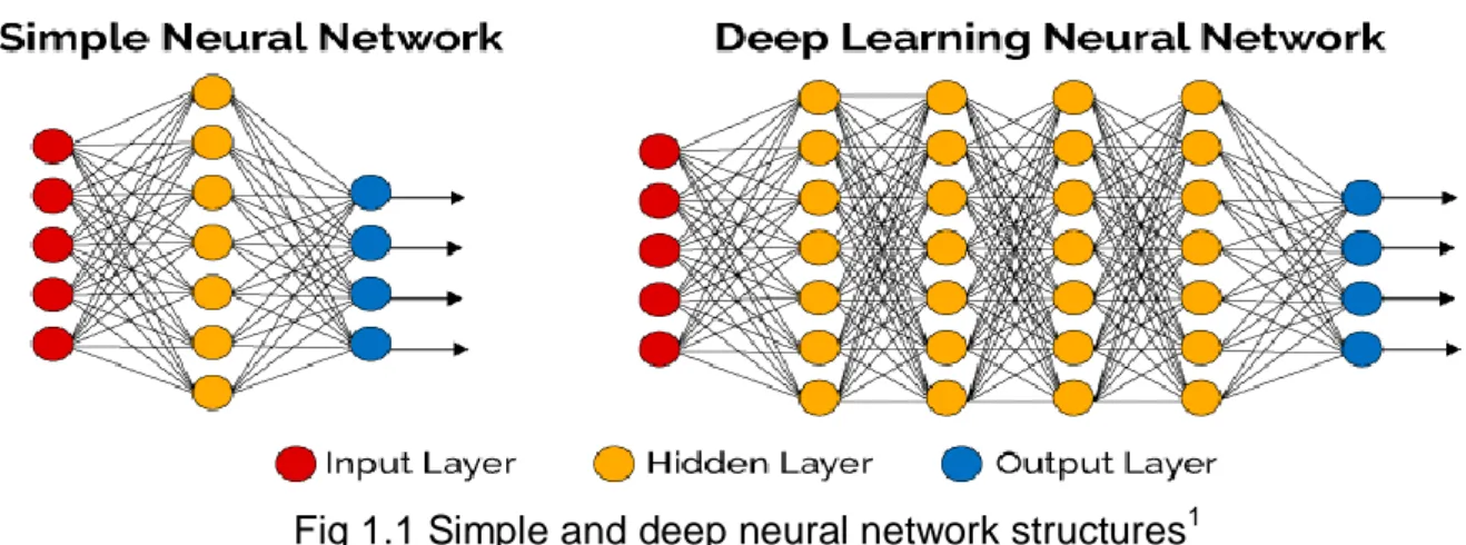
to the number of classes. Typically, a single linear output neuron is used to predict a continuous output. All connections in the network are lead from the input layer to the output layer, and it is possible to create deep networks by adding more hidden layers to which each neuron binds to each neuron in the following layer [17]. Deep learning provides a very strong framework for the supervised learning process. By adding more units to a layer, a deep network can represent increased complexity functions. It is easy to match an input vector to an output vector, with the help of human easily. But, that process can be accomplished through deep learning model with modeled large data sets and exemplary training samples [2]. To put it more simply, classical (simple) neural networks have only one hidden layer, whereas deep neural networks have more than one hidden layer (Figure 1.1).
Deep learning is based on learning from the representation of the data. When it comes to representation of an image; features can be considered such as a vector, edge sets of density values per pixel or special shapes. Some of these features represent data better. Besides, deep learning algorithms can learn their features throughout the learning process.
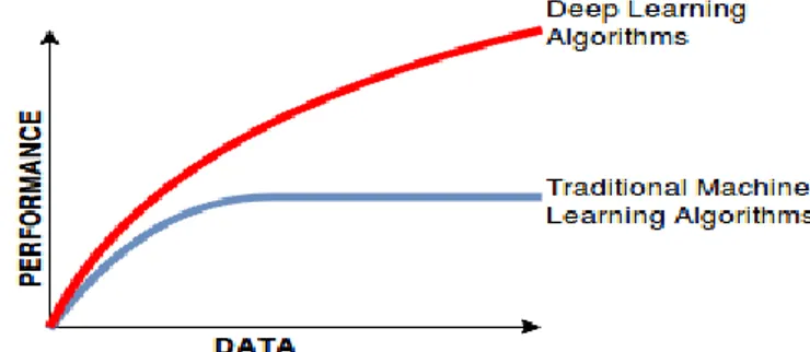
In recent years, increase in Big Data and the ability to create more successful systems has made deep learning a topic that is frequently studied in the last roads. With deep learning, the success performance of older machine learning algorithms have increased according to Figure 1.2.
Fig 1.1 Simple and deep neural network structures1
4
Fig 1.2 Data size and performance comparison of deep learning and traditional machine learning algorithms2
1.3 RNN and LSTM Background
Recurrent neural networks or RNNs are a family of neural networks to make a sequential data meaningful [2]. RNN is a deep neural network where the links of units form a directed loop [3]. Since the inputs are processed as a sequence, the repetitive calculation is performed in hidden units with a cyclic connection. That's why memory is stored indirectly in hidden units called state vectors, and the output for the current input is calculated by considering all previous inputs using these state vectors [4].
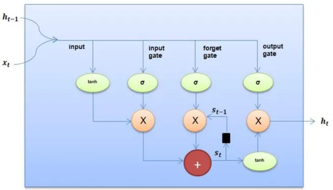
Long short-term memory (LSTM) model is based on recurrent neural network (RNN) architecture which remembers values at random intervals. The saved values do not change when the learned progress is made. RNNs allow forward and backward connections between neurons [1].
In the RNN and LSTM deep neural networks, inputs are represented by x, hidden units by h, and output units by y. For LSTM, the hidden unit h functions are the output unit. The RNN has a simpler structure than LSTM and lacks the gating process. All RNNs have feedback loops at the repetitive layer. Thus, over time they are provided to keep the information “in memory”. However, it is difficult to train standard RNNs to solve long-term interdependencies which require learning. This is because the gradient of the loss function gradually decreases over time.
2
Aditya Sharma. (2018). Differences Between Machine Learning & Deep Learning. https://www.datacamp.com/community/tutorials/machine-deep-learning
5
Fig 1.3 Long-Short Term Memory (LSTM) Architecture
LSTM units contain a “memory cell” that can hold information in memory for a time. A series of gates are used to control when the information is entered in memory when it is exited and when it has been forgotten. This architecture allows them to learn long term dependencies. Also, RNN has a single layer (tanh) and LSTM has four interactive layers.
First, on the left, there is a new sequence value , which is combined with the previous output from cell . The first step of this combined input through a tanh
layer. The second step is to pass this input through an input gate. An input gate is a layer of sigmoid active nodes whose output is multiplied by input. This sigmoid function can be moved to remove all unnecessary elements of the input vector. Also, a sigmoid function returns values between 0 and 1.
The next step in the LSTM network is the forget-gate. LSTM cells have an internal state that is This variable with a time-out delay is added to the input data to form an active iteration layer. Adding this instead of multiplication helps to reduce the risk of vanishing gradient. However, this iteration loop is controlled by a forget gate and it works in the same way as the input gate, but instead it helps the network
6
learn which status variables need to be "remembered" or "forgotten" [18].
Lastly, an output gate specifies which values actually pass through the , cell as an output (Figure 1.3).
The mathematics of the LSTM cell is defined as below:
In the Input Gate:
The input is scaled between -1 and 1 with using tanh activation function.
g = tanh( ) (1.1)
The input gate and previous cell output are expressed with and . is the input bias. This embedded input is multiplied by the output of the input gate which is defined as below:
i = σ( ) (1.2)
Then the input section output will be as below:
g ∘ i (1.3)
∘ operator expresses element-wise multiplication.
State Loop and Forget Gate:
The forget gate output is defined as:
f = σ( ) (1.4)
Then the previous state and f will be multiplied. After that, output from forget gate will be expressed as:
= ∘ f + g ∘ i (1.5)
7 The output gate is defined as below:
o = σ( ) (1.6)
As a result, final output will be:
= tanh( ) ∘ o) (1.7)
1.4 Decision Tree
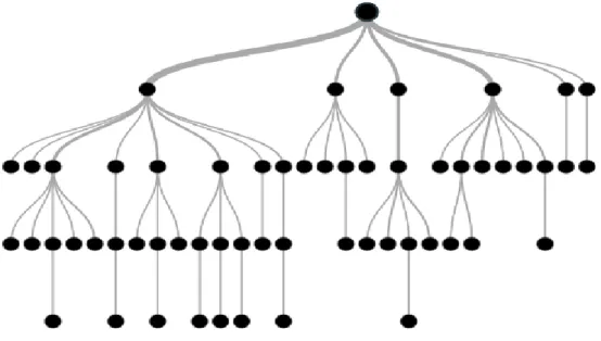
Tree-based learning algorithms are one of the most used supervised learning algorithms. In general, they can be adapted to the solution of all problems related with classification and regression. The decision tree algorithm is one of the data mining classification algorithm. They have a predefined target variable. In terms of their structure, they offer a top-down strategy (Figure 1.4). A decision tree has a structure which is used to divide a data set containing a large number of records into smaller clusters by applying a set of decision rules. In other words, it is a structure used by dividing large amounts of records into very small groups of records by applying simple decision-making steps.
8
Fig 1.4 Graphical representation of decision trees3
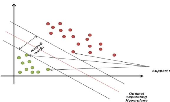
1.5 Support Vector Machine (SVM)
Support Vector Machines (SVM) is founded by Vladimir Vapnik and Alexey Chervonenkis in 1963 and it is a supervised learning algorithm based on statistical learning theory. Support Vector Machines are mainly used to optimally separate data from two classes. For this purpose, decision limits or in other words hyperplanes are determined (Figure 1.5). They are effective in high dimensional spaces. Also, they are effective when the number of dimensions is greater than the number of samples. The decision function uses several training points (support vectors). Therefore, memory is used efficiently.
3
9
Fig 1.5 Graphical representation of Support Vector Machines
1.6 K-Nearest Neighbors (kNN)
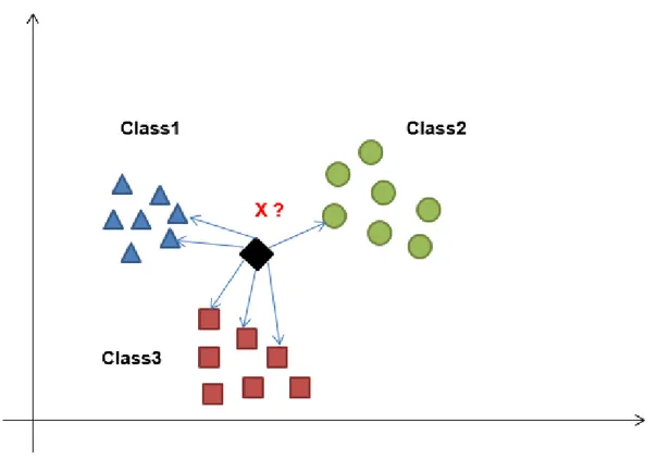
The k-nearest neighbor (kNN) algorithm is one of the supervised learning algorithms. It can be used to solve both classification and regression problems. The kNN algorithm was proposed in 1967 by T. M. Cover and P. E. Hart. The algorithm is used for gathering data from a sample set with defined classes. The distance of the new data to be included in the sample data set is calculated according to the existing data. So, k close neighborhoods (kNNs) are examined (Figure 1.6). kNN, is one of the most popular machine learning algorithm because it is robust againts to old, simple and noisy training data [19].
10
Fig 1.6 Graphical representation of kNN algorithm
1.7 Random Forest
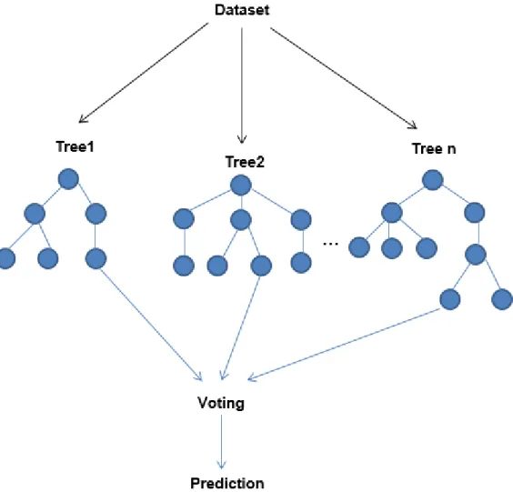
Random Forest (RF) is a supervised learning algorithm. It creates a forest, randomly. The forest founded is a collection of decision trees, often trained by the bagging method. The general idea of the bagging method is: combination of learning models increases the overall outcome. In simple words: a random forest creates multiple decision trees and combines them to achieve more accurate and stable prediction (Figure 1.7).
11
Fig 1.7 Graphical representation of Random Forest Algorithm
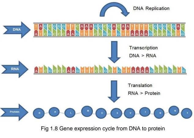
1.8 Biological Terminology and Background of microRNAs
Gene expression is the process of converting the instructions in the DNA into a functional product, e.g. a protein. When the information stored in the DNA is converted into instructions for making proteins or other molecules, this phenomenon is called "expression of the gene" or "gene expression". The system that regulates a cell's response to the changing environment is called gene expression. It functions as a volume control that increases or decreases the number of proteins produced as well as the release button that controls when proteins are produced [20]. There are two important stages of gene expression: transcription and translation (Figure 1.8).
12
Fig 1.8 Gene expression cycle from DNA to protein
Transformation of DNA into RNA is called transcription. The transformation of RNA into protein is called translation. The DNA alphabet consists of 4 characters. They are A (Adenine), G (Guanine), C (Cytosine), T (Thymine). Also, the RNA alphabet contains 4 characters. They are A (Adenine), G (Guanine), C (Cytosine), U (Uracil).
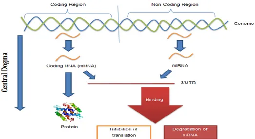
MicroRNAs (miRNAs) are the type of RNA. They have ~23 nucleotides length, and play gene-regulatory roles and they are responsible for biosynthesis of tissues in cells for many living organisms. On the mRNA, they bind partial complementary target sites and cause post-transcriptional repression or cleavage of mRNA (Figure 1.9). They inhibit the genesis of peptides and output proteins [1, 5]. miRNAs are known to be associated with many diseases such as cancer due to deformation in protein production and defects in the regulation of miRNA translation [6]. Besides, recent research is shown that gene regulation of neurodevelopmental and psychiatric disorders may be observable because of some kind of miRNAs [7, 8].
13
Many miRNA target sites are determined experimentally and computationally, but only a few are experimentally verified. Therefore, computational estimation of the function of miRNA targets is a competitive task to support a major effort in understanding gene regulation. [6, 9, 17].
Prediction of miRNA target sites is a compelling task in molecular biology and bioinformatics. It is an important step to understand the interaction of a miRNA with other genes and its functional position in regulatory mechanisms. Furthermore, the experimental determination of this relationship is laborious and long. Therefore, several studies have been conducted to understand the binding relationship between miRNA and mRNA given over the last fifteen years. In addition to DNA, the RNA has a 3 '(3 prime) and 5' (5 prime) end. This has to do with the direction in which the sequence is read. UTR stands for untranslated region.
Translation is the process of producing a protein from mRNA. As the name suggests, 3'UTR does not turn into a protein. The present methods generally take the miRNA sequence and the 3'UTR mRNA sequence and decide whether the given miRNA will recognize the mRNA as its target site [6]. miRNAs have a region of 7-8 nucleotides, called seeds, at the 5 'end, which is generally thought to direct recognition of the binding site in the 3'UTR target mRNA. Some experiments have proven the presence of a strong base pairing in verified miRNA target pairs.
In previous studies, the only prediction based on sequence complementarity produced a large number of false positives. As a result, many of the recent methods relied on a combination of various factors, such as sequence composition, seed match, site conservation, sequence complementarity, minimization of free energy in the miRNA-target duplex, and site accessibility. Recent research has shown that the use of machine learning and deep learning methods to solve the target binding site prediction problem improves the accuracy of prediction results.
14
Fig 1.9 Function of miRNA during the central dogma process
1.9 Related Works
There are several tools for miRNA target prediction. RNAhybrid (2006) is the first developed and score-based algorithm for the microRNA target site prediction problem. They use G:U base pairs in the seed region as feature [22]. miTarget (2006) they used 15 features e.g. (positions, free energy, AU matches, mismatches, total free energy, etc.). They used SVM Classifier for prediction [23]. EiMMo (2007), they present model the evolution of orthologous target sites in related species. They used Bayesian based learning [24]. miRecords (2009), they create a resource for animal miRNA-target interactions [25]. TargetSpy (2010), their method is based on machine learning and automatic feature selection using compositional, structural, and base pairing features [26]. miRmap (2013) combines thermodynamic, evolutionary, probabilistic and sequence-based features. Their model type is based on Regression [27]. mirMark (2014), uses experimentally verified miRNA targets as training sets and considers over 700 features. They used Random Forest based classifier [15]. TargetScan v7.0 (2015) [12] examines that canonical sites are more functional than non-canonical sites to understand miRNA binding sites. They extract 14 features and they train the data by using multiple linear regression models. They are reached 58.01% accuracy, 60.23% sensitivity, 59.22% specificity [1]. TarPmiR (2016) [11] developed a random-forest-based method to predict miRNA target sites. Their method is random-forest-based on scanning
15
miRNA on mRNA sequence to get the excellent seed-matching sites. They used six conventional features and seven of their own features, together. As a result, TarPmiR selects the site with the highest likelihood as the target site [1]. They achieved 74.46% accuracy, 73.68% sensitivity, 76.56% specificity.
MiRTDL (2016), is based on Convolutional Neural Network (CNN). They achieved 88.43% sensitivity, 96.44% specificity, and 89.98% accuracy [28].
DeepMirTar [10] is a recent method based on stacked de-noising auto-encoder deep learning method (SdA) to predict human miRNA-targets on the site level. They used three different feature representations to express miRNA targets, i.e. high-level expert designed features, low-level expert designed features and Raw-data-level designed features. Seed match, sequence composition, free energy, site accessibility, conservation, and hot-encoding are some of the examples of these features. They achieved 93.48% accuracy, 92.35% sensitivity, 94.79% specificity.
16
2. METHODS
In this chapter, in Section 2.1, the inference of the input function to train the model is explained. In Section 2.2, the developed deep neural network model structure is discussed. Section 2.3 provides information about the developed web application and a web server.
2.1 Input Representation
Preprocessing are performed before the data are given as input to the LSTM deep neural network. While the inputs are represented, two inputs consisting of miRNA and mRNA in the dataset are tried to be expressed as a single input.
2.1.1 Sequence Alignment and Needleman Wunsch Global Alignment Algorithm
Sequence alignment method is used to find similarity between two or more sequences. Sequence type might be DNA, RNA or protein sequences. Many biological mechanisms can be understood by sequence alignment methods. For instance; finding similar proteins allows predicting the function and structure of the proteins involved. The presence of similar sub-sequences in DNA allows the identification of regulatory elements. In sequence alignment, inputs are represented by two or more sequences over the same alphabet and outputs are represented by an alignment of these sequences. There are two types of sequence alignment methods; These are global and local alignment algorithms. In the global alignment algorithm, the sequences are aligned completely letter by letter. The global alignment algorithm is also known as the Needleman-Wunsch algorithm. On the other hand, in the local alignment algorithm, the similarity of the substrings in the two or more sequences are examined. The local alignment algorithm is also known as the Smith-Waterman algorithm (Figure 2.1).
17
Fig 2.1 Examples of Local and Global Sequence Alignment
In miRNA and related mRNA alignment, two molecules are complementarily bounded to each other. By complementary binding, the phenomenon to be described is that each pair of A-U, U-A, and G-C, C-G nucleotides are complementary to each other. For this reason, Needleman-Wunsch global complementary alignment algorithm is used in this study. Needleman-Wunsch algorithm is based on dynamic programming (Figure 2.2). The general use of this algorithm is used to align protein or nucleotide sequences. Genetic DNA, RNA sequences to reveal the similarity between each other.
The key logic of the algorithm is based on finding the maximum similarity between the two sequences.
Match: two characters are the same Mismatch: Two characters are different
Space: A character that corresponds to the space in the other array points should be determined and transactions should be made accordingly.
18
Fig 2.2 Needleman-Wunsch algorithm pseudocode
In the pseudocode of Needleman-Wunsch algorithm: M is the length of first sequence
N is the length of second sequence
S is the dynamic programming matrix of size M x N δ( ,-) is the score from aligning with a gap δ(-, ) is the score from aligning with a gap δ( , ) is the score from aligning with
Output: Optimal alignment score for aligning M and N
2.1.2 Proposed Input Representation
The obtained duplex sequence by using alignment of the miRNA sequence with a related target site on the mRNA sequence is used to feed the deep learning network. Duplexes for each miRNA pair and target site are aligned with the "Needleman - Wunsch" global complement alignment algorithm [13]. Thereafter, different alphabetic characters are used for the nucleotides corresponding to each A-U and G-C. G-U wobbles are ignored. Consequently, it is aimed to reduce the total number of characters in develoed LSTM network [1]. Each A-U pair is represented by “a, each U-A pair is indicated by“ b, each G-C pair is expressed by “c, each C-G pair is expressed by“ d, and all remaining pairs are expressed by “q (Figure 2.3, Figure 2.4).
19
Fig 2.3 Methodology used in input representation
Fig 2.4 Alignment of miRNA sequence (middle) mRNA binding site (top)
converted from a new
sequence of duplex formation (bottom).
2.2 The LSTM Network
In this section, the builded deep neural network architecture is explained with its components.
2.2.1 Embedded Vector Layer
The key idea behind the embedded vector is that each word used in a language may be represented by a set of numerical values (vectors).
20
First, each duplex sequence obtained by methodology, as discussed in (Section 2.1.2), converted the letter into the index. The character a, b, c, d, q are converted to index 0, 1, 2, 3, 4 respectively (Figure 2.5). In embedded vector, one-hot encoded words or index words are mapped to the dense word vectors. When finding embedded vector weights, discrete values are converted to continuous values. Embedded vector uses the TF - IDF (term frequency–inverse document frequency) method which is an information retrieval (IR) algorithm in the background. The TF * IDF method measures the frequency (TF) of the term and its inverse document frequency (IDF). Each word or term has its TF and IDF score. The product consisting of a term's TF and IDF points is called the TF * IDF weight of that term. The TF-IDF algorithm is used to search for a word in any content and give importance to the searched word according to the frequency it appears in the document. For term t in document D, the weight of term Wt,d in document d is given by the following formula:
Wt,d = TFt,d log (N/DFt) (2.1)
- N is the total number of documents in the dataset. - TFt,d is the number of occurrences of t in document d. - DFt is the number of documents containing the term t.
According to Figure 2.5, for the first character „a‟ in example duplex sequence:
TF(a) = 5 / 32 = 0,15625
IDF(a) = log(7820 / 5062) = 0,1889232
W(a) = (TF*IDF)(a) * (position of the character) = 0,15625 * 0,1889232 * 1 = 0,029551925
5 shows how many times the 'a' character repeats in a 32-long vector. 32 shows vector length. 7820 shows number of samples in the dataset 5062 shows how many times the „a‟ character repeats in all samples.
21
Fig 2.5 An example of proposed embedded vector representation
Before the data are learned and tested by the built deep neural network, the size of each duplex sequence, letter to index and embedded vector weights are fixed in the form of a vector of length 32.
2.2.2 Dropout Layer
Dropping-out aims to drop or remove variables that are input to layers in the neural network. It has the effect of making the nodes in the network more robust for inputs and simulating multiple networks with different network structures. Technically, in each training step, the individual nodes are removed from the network with 1-p probability, and a reduced network remains. The need for Dropout Layer is to reduce the possibility of overfitting data during training. A fully connected layer uses most of the parameters inefficient, and therefore, neurons
22
(a) (b)
Fig 2.6 Deep neural network structures with drop-out layer4
(a) Standard deep neural network structure
(b) Deep neural network structure obtained by applying drop-out process to (a)
develop interdependence between each other, which reduces the individual strength of each neuron during training and leads to overfitting of the training data (Figure 2.6). Besides, dropout is an approach in deep neural networks that relies on interdependent learning among smart neurons. Dropout method is one of the most common regularization methods used in deep learning.
2.2.3 Dense Layer
A dense layer is one of the layer in the neural network. Each neuron receives input from all neurons in the previous layer so that it is densely bounded. The layer has a weight matrix W, a bias vector b, and activations of the previous layer a. A dense layer is a fully connected neural network layer. The dense layer is used to modify the dimensions of the related vector. Mathematically, it applies a scaling, rotation, translation and transformation to the corresponding vector.
4
Amar Budhiraja. (2016). Dropout in (Deep) Machine learning.
ttps://medium.com/@amarbudhiraja/https-medium-com-amarbudhiraja-learning-less-to-learn-better-dropout-in-deep-machine-learning-74334da4bfc5
23
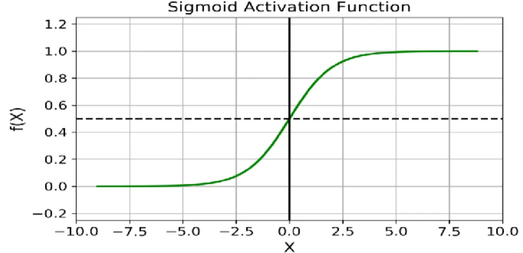
2.2.4 Sigmoid Activation Function
Fig 2.7 A coordinate representation of sigmoid activation function5
f(x) =
(2.2)
Sigmoid function is one of the most commonly used activation function. In contrast to the linear function, in the sigmoid function, the output of the activation function will always be within range (0,1) (Figure 2.7). Then it can be used in binary classification problems.
2.2.5 Binary Cross-Entropy Loss Function
Binary Cross-Entropy loss is used to measure the performance of a binary classification model whose output has a probability value between 0 and 1. As the predicted probability differs from the actual label, the loss of cross-entropy increases. For example, when the actual observation label is 1, it will predict the probability of 0.006 and result will be in a high loss value. An excellent model would be 0 log loss.
5
Sovit Ranjan Rath. (2019). Activation Functions in Neural Networks. https://debuggercafe.com/activation-functions-in-neural-networks/
24
Fig 2.8 A graphical representation of log loss and predicted probability6
What is meant in the Figure 2.8 is the range of possible loss values given with the correct observation. When the predicted probability is 1, the log loss gradually decreases. As predicted probability decreases, log loss increases rapidly.
2.2.6 Adam Optimizer
Adam is an optimization algorithm. It can be used instead of the classical stochastic gradient descent method to update recursive network weights based on training data. Adam is derived from adaptive moment estimation [21]. Adam Algorithm was presented by Diederik Kingmaand and Jimmy Ba in a paper titled “Adam: A Method for Stochastic Optimization” in 2015 [14]. Adam has been created by combining the best features of the AdaGrad and RMSProp algorithms to provide an optimization algorithm that can handle the sparse transition in noisy problems. Adam is easy to use where most of the default configuration parameters are good for the problem. Relatively low memory requirements are an advantage for the Adam algorithm.
6
25
2.2.7 Stochastic Gradient Descent (SGD) Optimizer
SGD is a widely used optimization technique in Machine Learning and Deep Learning. It can be used with most learning algorithms. A gradient is the slope of a function; mathematically, they can be defined as partial derivatives of a range of parameters based on their input. Gradient Descent can be defined as an iterative method that tries to minimize the cost function and is used to find the values of the parameters of a function.
What is meant by the word "stochastic" is a system or a process associated with a random probability. Thus, in the SGD, several random samples are selected instead of selecting all data set for each iteration. SGD uses only one sample to perform each iteration. The sample is mixed randomly and selected one is used to perform the iteration.
2.2.8 Adadelta Optimizer
Adadelta is derived from Adagrad and tries to reduce the aggression of Adagrad, by reducing the learning rate monotonously. This is done by keeping the window of the past accumulated gradient limited to some fixed size. At run time, the average depends on the previous average and the current gradient.
2.2.9 Proposed LSTM Network
In this architecture, the first layer is a Embedded layer, as described in Section 2.2.1, that is going to convert sequences into numerical embedded vectors. 32 vector length is used to represent each word in the embedded layer. In addition, the parameter "500" is used to specify the size of the vector range that defines the words to be embedded. The size of the output layers for each word is defined in this layer (Table 2.1).
As the second layer, Dropout Layer is used. The main purpose of using this layer is to prevent overfitting and eliminate garbage data. Drop-out percentage is
26
selected as 20%. The third layer is the LSTM layer with 1000 smart neurons. As the fourth layer Dropout Layer is used. Finally, since this problem is a binary classification problem, it is used a dense output layer with a single neuron and sigmoid activation functions is used to predict 0 (not target) or 1 (target). The main and higher level architecture of the study is given to Fig 2.12.
Since the problem is a binary classification problem, log loss is used as a loss function. In addition, the “Adam” algorithm is chosen as the optimizer. Adam is an optimization algorithm that recursively updates network weights in training data. Besides, the loss of validation is measured every 5 epochs to avoid over-fitting. If the validation loss is increased from the previous one, the early stop function is activated. As a consequently, the learning process is interrupted [1].
Table 2.1 Layers of proposed LSTM network
Layer Type Output Shape
Embedding (500,32)
Dropout_1 (500,32)
LSTM 1000
Dropout_2 1000
Dense 1
2.3 Implementation and Availability
The inputs (aligned duplex sequences) was extracted with python 3. After that pro-cess, the learning step was developed in Google Colaboratory environment using the keras library of python software language. In the web application, HTML5 and CSS3 were used in the frontend. To keep the data generated by the deep learning model, MySQL database was preferred. Also, PHP was used to manipulate data
27
between the MySQL and the frontend. The web server is accessible at https://mirna.atwebpages.com.
In the web application, the user is prompted to enter a microRNA sequence as an input (Figure 2.9).
When the user enters a microRNA sequence as an input, if the deep learning algorithm is able to correctly classify the target site of the related microRNA (has found the target site), all the target binding sites of the related microRNA on the mRNAs are shown in red color (Figure 2.10).
28
Fig 2.10 Example of microRNAs query result. Red site is the target site.
When the user enters a microRNA sequence as an input, if the deep learning algorithm has not found the target site of the related microRNA, the output is given as "target binding site is not found." (Figure 2.11).
29
30
3. EXPERIMENT AND RESULTS
In this chapter, Section 3.1 provides information about the dataset used in the study. In Section 3.2, the experimental results of the study are described in detail.
3.1 Dataset
Two different data sets were used in this study. DSet2 is taken from the Deep-MirTar repository [10]. In the first data set, 3905 negative data are generated using mock miRNAs. 3915 positive (experimentally validated miRNA – target duplexes) data are collected, 473 of them are obtained from mirMark data [15] and 3442 of them are obtained from CLASH data [11]. Totally there are 7820 samples. This set of data is preferred since there are many experimentally confirmed positive data. DSet1 is obtained from the [16]. This dataset contains 283 positive and 115 negative miRNA-mRNA duplex sequences. Totally there are 398 samples. These two datasets are convenient for comparison because they have different sizes. The size of the DSet1 dataset is smaller than the DSet2 dataset [1]. Therefore, LSTM based approach is used to measure the prediction performance of different datasets in different sizes.
3.2 Emprical Results 3.2.1 Evaluation Criteria
To obtain the quality of prediction performance of proposed methods, the proposed methods and existing approaches for miRNA target prediction are compared. As an evaluation metric, accuracy, sensitivity, specificity, F1 score, AUC (Area Under Curve) are used.
31
Fig 3.1 Confusion matrix for binary classification
Given the confusion matrix in Figure 3.1, discussed metrics are described by the following equations: (3.1) (3.2) (3.3) (3.4)
Also, TPR (True Positive Rate) and FPR (False Positive Rate) are defined by the following equations: (3.5) (3.6)
32
3.2.2 Prediction Results
3.2.2.1 Prediction Results of DSet1
Thirty four different methods were used to test DSet1 (Table 3.2). The reason for trying thirty four different methods is to advance the work of Oğul et al [16]. Therefore, in addition to the data pre-processing method used in Oğul et al [16] study, it is intended to predict the target sites of the miRNA by using LSTM based learning method. From DS1_M1 to DS1_M30 method in Figure 3.2, performance of the deep learning system is measured according to different system hyperparameters. Additionally, there is used data pre-processing and it is attempted to set up a classification model that performed a miRNA target site prediction. Besides, with the help of DSet1, it is tried to classify the miRNA target site with using some simple machine learning methods. In the DS1_M31, SVM is used on DSet1. In the DS1_M32, DT is used on DSet1. In the DS1_M33, kNN is used on DSet1. In the DS1_M34, RF is used on DSet1.
Last of all, the results of thirty four methods are compared with using five metrics which are sensitivity, specificity, accuracy (ACC), AUC (Area under the curve) and F1 score [1].
33
Fig 3.2 The framework about proposed methods
DS1_M1 to DS1_M30
34
Firstly, from DS1_M1 to DS1_M30 the dataset is randomly mixed. After that, LSTM based model is performed by determining the test split size as 0.1. Hence, fourty randomly selected test data are collected. 5 metrics were considered to evaluate success criterion: sensitivity, specificity, accuracy (ACC), AUC and F1 score [1].
In Table 3.1, the performance criteria of the built LSTM model is given according to Method Name, Batch Size, Neuron Size, Input Length, Loss Function, and Optimizer as system parameters. As the results show, DS1_M1 gave the best result by using 4 batch size, 100 neuron size, 32 input length, binary cross-entropy loss functions and Adam optimizer. Input length and loss function system hyperparameters are not tested for different values because in the preprocessed dataset, the longest sized input sample is 32 in length. Furthermore, since the problem discussed is a binary classification problem, binary cross-entropy loss is preferred. According to Table 3.1, DS1_M1 method gives the best results, the increase in the number of neurons used in small size datasets decreases the success of the system. In other words, increase in the complexity of the system affects the performance negatively. In general, the best results are obtained with Adam optimizer. Also, 4 batch size gave better results than 8.
35
Table 3.1 Methods applied based on different system hyperparameter configurations on DSet1 Method Name Batch Size Neuron
Size Optimizer ACC TPR TNR F1 AUC
DS1_M1 4 100 adam 82,50 100 30,00 89,55 77,00 DS1_M2 4 250 adam 77,31 93,76 76,78 81,11 74,28 DS1_M3 4 500 adam 77,61 83,14 77,12 65,18 74,79 DS1_M4 4 1000 adam 55,44 86,61 61,26 67,70 71,77 DS1_M5 4 1500 adam 51,72 85,88 60,60 64,48 59,53 DS1_M6 4 100 ada-delta 71,62 74,56 64,70 66,51 78,82 DS1_M7 4 250 ada-delta 74,99 71,14 71,23 57,57 76,70 DS1_M8 4 500 ada-delta 62,41 74,12 70,41 59,23 77,47 DS1_M9 4 1000 ada-delta 64,18 70,46 66,67 60,06 72,33 DS1_M10 4 1500 ada-delta 54,66 81,98 31,15 44,19 63,21 DS1_M11 4 100 SGD 64,77 55,12 51,16 59,92 64,88 DS1_M12 4 250 SGD 59,46 59,31 57,28 64,12 71,71 DS1_M13 4 500 SGD 57,86 68,82 53,33 66,69 66,53 DS1_M14 4 1000 SGD 54,44 69,08 33,76 57,75 61,38 DS1_M15 4 1500 SGD 53,99 77,71 35,62 51,85 66,22 DS1_M16 8 100 adam 81,44 96,94 27,79 84,15 78,87 DS1_M17 8 250 adam 77,46 81,61 80,92 81,18 78,15 DS1_M18 8 500 adam 75,82 81,61 73,74 77,01 76,68 DS1_M19 8 1000 adam 72,31 75,75 85,58 60,43 78,95 DS1_M20 8 1500 adam 52,51 71,24 20,01 51,71 61,89 DS1_M21 8 100 ada-delta 72,25 84,85 71,81 75,49 81,66 DS1_M22 8 250 ada-delta 71,27 85,17 67,58 81,23 79,63 DS1_M23 8 500 ada-delta 63,76 85,17 61,26 79,30 75,55 DS1_M24 8 1000 ada-delta 64,85 81,81 66,80 73,44 71,52 DS1_M25 8 1500 ada-delta 67,67 86,09 45,16 51,35 74,32 DS1_M26 8 100 SGD 64,76 76,75 71,81 57,78 73,37 DS1_M27 8 250 SGD 64,76 76,75 71,81 57,78 73,37 DS1_M28 8 500 SGD 62,46 73,48 69,94 54,67 70,04 DS1_M29 8 1000 SGD 63,48 78,62 73,56 79,91 76,62 DS1_M30 8 1500 SGD 54,93 74,33 44,36 72,20 64,48
36
Table 3.2 Used dataset and method informations about proposed methods
Method Name Dataset Method
DS1_M1 – DS1_M30 DSet1 Preprocessing + LSTM
DS1_M31 DSet1 SVM
DS1_M32 DSet1 DT
DS1_M33 DSet1 kNN
DS1_M34 DSet1 Random Forest
Although similar data preprocessing steps are applied in DS1_M33 and Oğul et al. [16] methods, DS1_M33 gives better results in terms of ACC, TPR, and F1 score. While method DS1_M33 is better than method Oğul et al. [16] in learning positive data, method Oğul et al. [16] is better than method DS1_M33 in the scope of learning negative data. According to the results, developed LSTM model yields better results in some respects than method Oğul et al. [16], but also reveals poor results in some metrics (Table 3.3, Figure 3.3).
Table 3.3 Classification results of the best LSTM model (DS1_M1) and other basic machine learning methods on the DSet1
Method Name ACC TPR TNR F1 AUC DS1_M1 82,50 100 30,00 89,55 77,00 DS1_M31 76,75 84,02 37,09 85,9 60,6 DS1_M32 70,00 84,80 15,00 82,40 44,60 DS1_M33 85,50 89,3 64,51 91,12 77,80 DS1_M34 85,00 100 0,005 91,8 81,1 Oğul et al. [16] 84,60 86,70 73,70 87,80 95,00
37
Fig 3.3 A box-plot representation of evaluation metrics about proposed methods and related works
38
Fig 3.4 Illustration of the accuracy and loss values of DS1_M1. (a) Training and validation accuracy of the model during the learning process. (b) Training and validation loss of the model during the learning process.
Interrupted point of the learning process is shown in Fig 3.4. At this stage, according to the early stopping function, the learning process is terminated.
(a)
(b)
39
Fig 3.5 ROC curve of DS1_M1 generated by LSTM model on the training set
As far as known, the best classification has the largest area under the curve. In the Receiver Operating Characteristics (ROC) curve, the false positive ratio (Specificity) and actual positive ratio (Sensitivity) are plotted for different cut-off points. Each point in the ROC curve shows a sensitivity/specificity pair corresponding to the given decision threshold. A test with the best separation has a ROC curve passing through the upper left corner (100% specificity, 100% precision). So, the general accuracy of the test increases when the ROC curve approaches to the upper left corner. In this thesis study, the ROC Area is founded as 0.77 for DS1_M1 (Figure 3.5).
40
3.2.2.2 Prediction Results of DSet2
Totally there is used thirty five different methods. In the first method which name is DS2_M1, without doing any feature extraction, raw dataset in [10] is given directly to the proposed LSTM model to predict miRNA targets. From DS2_M2 to DS2_M31, (Figure 3.6) the DSet2 was used. Also in each method, performance of the developed deep learning model is measured in terms of different system hyperparameters. Additionally, there is used data pre-processing and attempted to build up a classification model which performed a miRNA target site prediction problem [1]. In the DS2_M32, SVM is used on DSet2. In the DS2_M33, DT is used on DSet2. In the DS2_M34, kNN is used on DSet2. In the DS2_M35, RF is used on DSet2 (Table 3.5).
As a consequently, the results of thirty five methods are compared by using five metrics which are sensitivity, specificity, accuracy (ACC), AUC (Area under the curve) and F1 score.
Fig 3.6 The framework about proposed methods
DS2_M2 to DS2_M31
41
Firstly, raw dataset is randomly mixed. After that, LSTM model is performed by determining the test split size as 0.1, so that 782 randomly selected test data are gathered.
In Table 3.4, the performance criteria of the builded LSTM model are given according to Method Name, Batch Size, Neuron Size, Input Length, Loss Function and Optimizer system parameters. Based on these results, DS2_M5gave the best result by using 64 batch size, 1000 neuron size, 32 input length, binary cross-entropy loss function and adam optimizer. Input length and loss function system hyperparameters are not tested for different values since in the preprocessed dataset the longest sized input sample is 32 in length. Furthermore, since the problem discussed is a binary classification problem, binary cross-entropy loss is preferred. According to the Table 3.4, DS2_M5 method gives the best results. So, increase in the number of neurons used in large size datasets increases the success of the system. However, when the number of neurons is 1500, performance of the model decreased because of the model complexity. In general, best results are obtained with the adam optimizer. In addition, the ada-delta optimizer is at least as successful as adam optimizer. Also, 64 batch size gave better results than 128.
42
Table 3.4 Methods applied based on different system hyperparameter configurations Method Name Batch Size Neuron
Size Optimizer ACC TPR TNR F1 AUC DS2_M2 64 100 adam 84,02 82,38 85,60 83,57 91,00 DS2_M3 64 250 adam 85,81 86,26 85,35 85,71 92,18 DS2_M4 64 500 adam 60,61 33,41 87,12 45,58 80,73 DS2_M5 64 1000 adam 87,34 91,45 83,33 87,70 92,59 DS2_M6 64 1500 adam 55,12 93,78 17,42 67,34 58,65 DS2_M7 64 100 ada-delta 78,26 71,50 84,84 76,45 84,78 DS2_M8 64 250 ada-delta 85,29 83,41 87,12 84,84 89,96 DS2_M9 64 500 ada-delta 84,14 79,01 89,14 83,10 89,74 DS2_M10 64 1000 ada-delta 86,31 88,64 82,54 85,01 89,13 DS2_M11 64 1500 ada-delta 60,19 93,56 0,22 34,87 54,61 DS2_M12 64 100 SGD 60,87 60,88 61,61 60,80 77,12 DS2_M13 64 250 SGD 60,10 68,13 52,52 62,84 78,67 DS2_M14 64 500 SGD 66,98 72,22 52,65 70,32 81,10 DS2_M15 64 1000 SGD 50,38 88,60 18,43 65,08 74,75 DS2_M16 64 1500 SGD 59,69 88,55 31,50 21,58 64,86 DS2_M17 128 100 adam 82,23 83,93 80,55 82,33 90,15 DS2_M18 128 250 adam 82,64 83,33 82,29 85,61 90,55 DS2_M19 128 500 adam 70,08 44,00 88,47 54,70 78,75 DS2_M20 128 1000 adam 61,13 38,60 83,08 49,50 55,69 DS2_M21 128 1500 adam 57,05 91,44 10,80 71,17 63,66 DS2_M22 128 100 ada-delta 78,52 81,08 78,78 79,94 83,99 DS2_M23 128 250 ada-delta 86,11 87,81 80,94 85,44 90,68 DS2_M24 128 500 ada-delta 79,67 82,80 89,33 84,03 90,95 DS2_M25 128 1000 ada-delta 83,58 88,77 81,08 76,74 90,95 DS2_M26 128 1500 ada-delta 56,76 91,90 26,61 36,83 62,44 DS2_M27 128 100 SGD 66,34 57,57 66,66 47,79 71,58 DS2_M28 128 250 SGD 64,22 73,56 59,17 63,64 86,90 DS2_M29 128 500 SGD 62,94 77,46 58,87 67,76 83,80 DS2_M30 128 1000 SGD 51,56 84,57 22,11 70,69 72,21 DS2_M31 128 1500 SGD 64,69 88,76 35,53 27,55 60,41
43
Table 3.5 Used dataset and method informations about proposed methods
Method Name Dataset Method
DS2_M1 DSet2 Raw Dataset + LSTM
DS2_M2 - DS2_M31 DSet2 Preprocessing + LSTM
DS2_M32 DSet2 SVM
DS2_M33 DSet2 DT
DS2_M34 DSet2 kNN
DS2_M35 DSet2 Random Forest
In DeepMirTar, they represent the miRNA-mRNA duplexes with using 750 different features. Some of these features are free energy, seed match, sequence composition, site accessibility. Proposed methods represent the miRNA-mRNA pairs based on a probabilistic approach. In the learning phase, they used SdA (Stacked denoising auto-encoder) based on deep neural network. They split dataset as 60% training data, 20% validation data and 20% test data. Besides, in this work, the dataset divided into 90% training data and 10% test data. They optimized the hyperparameters via grid-search method. On the other hand, there are optimized hyperparameters with random search method. They examine learning rate as 0.01 and batch size as 10. In this work, learning rate is determined
Table 3.6 Classification results of the best LSTM model DS2_M5 and other basic machine learning methods on the DSet2
Method Name ACC TPR TNR F1 AUC DS2_M5 87,34 91,45 83,33 87,70 92,59 DS2_M32 81,62 78,50 84,70 81,00 81,60 DS2_M33 81,39 85,58 82,59 81,39 87,68 DS2_M34 86,71 74,80 98,50 84,90 88,40 DS2_M35 83,25 81,73 94,20 80,70 85,40 DeepMirTar 93,48 92,35 94,79 93,48 97,93 TargetScan v7.0 58,01 60,23 59,22 22,50 67,25 TarPmiR 74,46 73,68 76,56 28,40 80,21
44
as 0.1 and batch size as 64. Also, they used 1500 memory units (smart neurons). In this study, 1000 smart neurons is used in the LSTM layer [1].
As a result, DeepMirTar method gives better results than proposed methods since it has a strong optimization of hyperparameters, a more complex deep neural network structure and a strong input representation on the first layer of the deep network (Table 3.6, Figure 3.7).
Fig 3.7 A box-plot representation of evaluation metrics about proposed methods and related works
45
Fig 3.8 Illustration of the accuracy and loss values of DS2_M5. (a) Training and validation accuracy of the model during the learning process. (b) Training and
validation loss of the model during the learning process.
The interrupted point of the learning process is shown in (Fig 3.8). At this stage, according to the early stopping function, the learning process is finished.
Interrupted Point (a)
46
Fig 3.9 ROC curve of DS2_M5 method generated by LSTM model on the training set.
47
4. CONCLUSION and FUTURE WORK
In this thesis, a deep learning based algorithm is developed to predict which site is microRNA will bind to in mRNA. In addition by using existing input extraction, a deep learning method based on RNN - LSTM is used to solve this problem. Also, the generated LSTM neural network model and previous problem-specific studies are compared with each other according to various evaluation metrics.
Developed LSTM model is extensively compared with different simple machine learning methods. Furthermore, performance measures on different size datasets of the used methods are compared with each other.
Besides all of these, an easy-to-use web application is developed with an interface for people working in the field of life sciences. They can see the potential target binding sites of a miRNA sequence by using this application.
Traditional machine learning based approaches are developed via window-based scanner over the mRNA sequence to examine the target binding site. Deep learning based LSTM model gives more significant results because of input sequence includes lots of different characters and their lengths are varied. Furthermore, the model requires a long-term context or dependencies between each different character in the input sequence. Therefore, the LSTM-based model has succeeded in overcoming these problems.
The results have shown that the method can outperform conventional shallow machine learning techniques when larger datasets are available.
In the future works, to get better results, a hybrid method can be considered by combining CNN and RNN - LSTM methods. Canonical and non-canonical sites can be considered also. The number of layers can be increased by using LSTM based model. G-U wobbles can be considered at the pre-processing step.
48
REFERENCES
[1] PAKER A., OĞUL H., mirLSTM: A Deep Sequential Approach to MicroRNA Target Binding Site Prediction, Computer and Information Science Communications, vol.1062, p.38-44, 2019.
[2] GOODFELLOW, I., BENGIO, Y., COURVILLE, A., Deep learning, 1th Edition, MIT Press, 2016.
[3] LEE, B., BAEK, J., PARK, S., YOON, S: deepTarget: end-to-end learning framework formicroRNA target prediction using deep recurrent neural networks, Proceedings of the 7th ACM International Conference on Bioinformatics, Computational Biology and Health Informatics, p.434–442, 2016.
[4] LECUN, Y., BENGIO, Y., HINTON, G., Deep learning, Nature, vol.521, p.436-444, 2015.
[5] BARTEL, D., MicroRNAs: Target Recognition and Regulatory Functions, Cell, vol.136, no.2, p.215-233, 2009.
[6] OĞUL H., AKKAYA M.S., Data integration in functional analysis of microRNAs, Current Bioinformatics, vol.6, p.462-472, 2011.
[7] BARTEL, D.P., MicroRNAs: Genomics, Biogenesis, Mechanism and Function, Cell, vol.116, no.2, p.281-297, 2004.
[8] XU, B., HSU, P., KARAYIORGOU, M., GOGOS, J., MicroRNA dysregulation in neu-ropsychiatric disorders and cognitive dysfunction, Neurobiology of Disease, vol.46, no.2, p.291-301, 2012.
[9] DEDE D., OĞUL H., TriClust: A Tool for Cross-Species Analysis of Gene Regulation, Molecular Informatics, vol.33, no.5, p.382-387, 2014.