Başlık: Survival probabilities for compound binomial risk model with discrete phase-type claimsYazar(lar):TUNCEL, AltanCilt: 65 Sayı: 2 Sayfa: 011-022 DOI: 10.1501/Commua1_0000000755 Yayın Tarihi: 2016 PDF

(1)

D O I: 1 0 .1 5 0 1 / C o m m u a 1 _ 0 0 0 0 0 0 0 7 5 5 IS S N 1 3 0 3 –5 9 9 1

SURVIVAL PROBABILITIES FOR COMPOUND BINOMIAL RISK MODEL WITH DISCRETE PHASE-TYPE CLAIMS

ALTAN TUNCEL

Abstract. Due to having useful properties in approximating to the other distributions and mathematically tractable, phase type distributions are com-monly used in actuarial risk theory. Claim occurrence time and individual claim size distributions are modelled by phase type distributions in literature. This paper aims to calculate the survival probabilities of an insurance com-pany under the assumption that compound binomial risk model where the individual claim sizes are distributed as discrete Phase Type distribution.

1. Introduction

Compound binomial risk model is …rst proposed by Gerber [8] to describe the surplus process of an insurance company. Compound binomial risk model can be described as a special case of discrete time version of the risk model. This model was studied by Shiu [16], Willmot [20] and Dickson [5]. Recently, Liu et. al. [11], Liu and Zhao [12], Eryilmaz [7], Li and Sendova [10], Tuncel and Tank [19] and Tank and Tuncel [17] have studied some extensions of compound binomial risk model. Stanford and Stroinski [15] calculated …nite time ruin probabilities for phase type claim size by recursive methods. Wu and Li [21] studied on discrete time Sparre-Anderson risk model for phase type claims.

The surplus process of an insurance company fUt; t 2 Ng is de…ned as

Ut= u + ct t

P

i=1

Yi, t = 0; 1; ::: (1.1)

with U0= u (initial surplus), the periodic premium is c and Yi is the claim amount

in related period. Suppose that Iibe a indicator function which represents the claim

occurrence where Ii’s are independent and identically distributed (i.i.d.). That is

Ii= 1 with probability p if a claim occurs in period i and Ii= 0 with probability

q, otherwise. For i 1, de…ne

Received by the editors: February 09, 2016, Accepted: April. 06, 2016.

2010 Mathematics Subject Classi…cation. Primary 91B30, 62P05; Secondary 47N30, 97K80. Key words and phrases. Compound binomial risk model, phase-type claims, non-homogenous claim occurrence, survival probabilities.

c 2 0 1 6 A n ka ra U n ive rsity C o m m u n ic a tio n s d e la Fa c u lté d e s S c ie n c e s d e l’U n ive rs ité d ’A n ka ra . S é rie s A 1 . M a th e m a t ic s a n d S t a tis tic s .

(2)

Yi = Xi ; Ii= 1

0 ; Ii= 0 (1.2)

Here, the random variable Xi strictly positive and fXi; i 1g forms a sequence

of i:i:d: random variables with probability mass function (p.m.f) f (x) = P (X = x):Under these assumptions Eq. (1.1) can be rewritten as

Un = u + n N n_P i=1

IiXi, n = 0; 1; ::: (1.3)

where Nnis the total claim number up to time n-th: The compound binomial model

can be orally de…ned as a binomial processes with independent increments for claim occurrences. Then the distribution of Nn random variables is assumed binomially

distributed. That is

P (Nn= k) = n

k p

k_qn k_{; k = 0; 1; :::; n}

Let W1denote the time until …rst claim appearance, W2denote the time between

…rst and second claims and more generally Wn denote the time between (n 1)st

and n-th claims. Thus W1; W2; :::; Wn can be thought as sequence of i.i.d. random

variables with geometric distribution

P (Wn= t) = P (I1= 0; :::; It 1= 0; It= 1) = pqt 1, t = 1; 2; ::: (1.4)

For an insurance company, ruin occurs at the …rst time that the surplus reaches to zero or below to zero. Thus the time of ruin, the ultimate probability of ruin and the …nite time probability of ruin are de…ned as follows

T = inffUt 0; t = 1; 2; :::g: (1.5)

(u) = P (T < 1jU0= u) (1.6)

(u; n) = P (T _njU0= u) (1.7)

respectively, where the initial surplus U0is u. Complement of Eq. (1.7) is described

as follows

(u; n) = 1 (u; n)

= P (Ut> 0; t = 1; 2; :::; n) (1.8)

and interpreted as the …nite time survival (non-ruin) probability. It is clear that, for n0> 0

(u1; n0) (u2; n0)

where u1 u2.

Supposing that net pro…t condition is p _X < 1:Under this condition is not certain to occur eventually Eryilmaz [7] :

Recursive formula for survival (non-ruin) probability when the claim occurrences are nonhomogeneous in the compound binomial risk model is given by Tuncel and

(3)

Tank [19]. Survival (non-ruin) probabilities after a de…nite time period of an insur-ance company in a discrete time model based on non-homogenous claim occurrences is studied by Tank and Tuncel [17]. In their studies, the distribution of Nn given

as P (Nn= k) = 8 > > > < > > > : pnP (Nn 1= k 1) + qnP (Nn 1= k) ; 1 k n 1 n Q i=1 qi ; k = 0 n Q i=1 pi ; k = n (1.9)

where P (Ii = 1) = pi and P (Ii = 0) = 1 pi = qi for i 1. Claim occurrence

probabilities may subject to be di¤erent between each other under the model as-sumption which has been given in Eq. (1.3). The distribution of the Nn random

variable can be stated by using the recursive formulas as given in Eq (1.9). Chen et. al. [4] discussed another recursive formula for computing P (Nn= k) . But this

formula is occasionally not stability of the distribution when pi’s are close to 1 and

n is large. The reader is refered to Chen et. al. [4] for the details.

Tuncel and Tank [19] have proposed the distribution of T random variable as

(1;n)_{(u) =} 8 < : 1 ; n = 0 n P t=1 pt t 1_Q i=1 qi u+t 1_P x=1 f (x) (t+1;n t)(u + t x) + n Q i=1 qi ; n > 0 (1.10) with non-homogenous claim occurrence probabilities for compound binomial risk model in related time periods. In here (t+1;n t)represent ruin time after the t-th period.

2. Discrete Phase-type distributions

The …rst studies of Phase-Type distributions is appeared at the …rst decade of 20th century. However the …rst modern study on the Phase-Type distributions, shortly written as PH distribution, was introduced by Neuts([13] ; [14]). After that, the PH distributions has become popular in di¤erent areas such as applied probability and actuarial risk theory. PH distributions can be either continuous or discrete. In this paper discrete version of the PH distribution is studied.

Discrete PH distributions may describe the time until absorption in a discrete time Markov chain with a …nite number of transient states and one absorbing state. Consider an (m + 1) absorbing discrete time Markov Chain with state space f0; 1; :::; mg and let state "0" be the absorbing state. Namely the …rst m state are transient and the last state is absorbing. In this case transition probability matrix is

P= T t

(4)

where T is a square sub-stochastic matrix of dimension m and all elements are between 0 and 1. t0 _{= (t}

10; :::; tm0) is a column vector and 0 is a row vector.

Let initial state distribution be = ( 0; 1; :::; m) and m

P

i=1

i = 1. We denote by

X random variable of the time to reach to absorbing state m + 1. In this case the distribution of X is called a discrete PH distribution which is represented by ( ; T). Even if the Markov chain starts from the absorption state "0", it is also possible to apply the discrete PH distribution for positive individual claim size Xi

i = 1; 2; :::. Furthermore it is also known that t = (I T)1; where I is identity matrix of dimension m m and 10 _{= (1; :::; 1) :}

The cumulative distribution function of X is then given by

F (x) = P (X x) = 1 Tx10 for x = 0; 1; 2; ::: (2.1) and its probability mass function is

f (x) = P (X = x) = Tx 1tfor x = 1; 2; ::: (2.2) The expected value of X can be computed the form of

E(X) = (I T) 110

The family of discrete PH distributions is closed under convolution. Note that, some useful properties of the discrete PH distributions make it attractive for risk modelling studies in actuarial sciences.

Suppose that X and Y are two independent discrete random variables that have phase type distributions with representations ( ; T) and ( ; D) respectively. Then, the distribution of X + Y turns into P H ( ; C) where

= 0

C= T t

0 D

More details on discrete PH distributions may be found in Asmussen [1], Bladt [2], Breuer and Baum [3], Drekic [6] ; Latouche and Ramaswami [9], Tank and Eryilmaz [18].

3. Numerical illustration

In this section, we present numerical illustration when individual claim sizes are arisen from zero-truncated geometric distribution which is PH distribution for m = 2. Let = (1; 0) ; t = (0; 1 ):

T= 1

0

In this case from Eq. (2.2), probability mass function is

P (X = x) = 1 0 1

0

x 1

0

(5)

This distribution given by Eq. (3.1) is known to be geometric distribution of order "2" Eryilmaz [7]. Let de…ne cases with non-homogenous claim occurrence proba-bilities in each periods as follows:

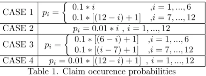
CASE 1 pi = 0:1 i ,i = 1; :::; 6 0:1 [(12 i) + 1] ,i = 7; :::; 12 CASE 2 pi= 0:01 i , i = 1; :::; 12 CASE 3 pi= 0:1 [(6 i) + 1] ,i = 1; :::; 6 0:1 [(i 7) + 1] ,i = 7; :::; 12 CASE 4 pi= 0:01 [(12 i) + 1] , i = 1; :::; 12

Table 1. Claim occurence probabilities

In Case 1, it can be seen that the probabilities of claim occurrences are increasing for …rst 6 periods from 0:1 to 0:6 and after that it is decreasing for last 6 periods from 0:6 to 0:1. In Case 2, it can be seen that the probabilities of claim occurrences are increasing from 0:01 to 0:12 for 12 periods. In Case 3, probabilities of claim occurrences are decreasing for …rst 6 periods from 0:6 to 0:1 and after that it is increasing for last 6 periods from 0:1 to 0:6. Finally, in Case 4, the probabilities of claim occurrences are decreasing from 0:12 to 0:01 for 12 periods.

So, survival probabilities are calculated and presented in Table 2 - Table 13 for di¤erent values, which are probability of claims, by Eq. (1.10) when P (Ii= 1) =

pifor i = 1; 2; : : : ; 12. n u = 1 u = 2 u = 3 u = 4 u = 5 u = 6 1 0:9000 0:9640 0:9768 0:9896 0:9942 0:9972 2 0:8352 0:9094 0:9509 0:9727 0:9854 0:9920 3 0:7505 0:8621 0:9139 0:9512 0:9710 0:9835 4 0:6870 0:7966 0:8720 0:9187 0:9502 0:9692 5 0:5995 0:7321 0:8124 0:8766 0:9177 0:9470 6 0:5238 0:6431 0:7435 0:8152 0:8720 0:9114 7 0:4363 0:5661 0:6624 0:7490 0:8140 0:8664 8 0:3845 0:4990 0:6021 0:6887 0:7629 0:8219 9 0:3464 0:4598 0:5576 0:6475 0:7234 0:7877 10 0:3271 0:4347 0:5323 0:6209 0:6986 0:7646 11 0:3168 0:4229 0:5189 0:6075 0:6853 0:7523 12 0:3134 0:4186 0:5142 0:6025 0:6805 0:7477 Table 2. Survival probabilities for = 1=5 in Case 1

(6)

n u = 1 u = 2 u = 3 u = 4 u = 5 u = 6 1 0:9000 0:9160 0:9256 0:9352 0:9433 0:9504 2 0:7488 0:7789 0:8044 0:8272 0:8473 0:8651 3 0:5795 0:6232 0:6609 0:6954 0:7264 0:7544 4 0:4221 0:4698 0:5133 0:5539 0:5915 0:6264 5 0:2874 0:3315 0:3733 0:4137 0:4524 0:4894 6 0:1803 0:2153 0:2502 0:2851 0:3197 0:3539 7 0:1128 0:1385 0:1650 0:1925 0:2206 0:2493 8 0:0779 0:0973 0:1177 0:1394 0:1621 0:1857 9 0:0594 0:0749 0:0915 0:1094 0:1283 0:1483 10 0:0494 0:0626 0:0770 0:0925 0:1091 0:1267 11 0:0442 0:0562 0:0693 0:0835 0:0988 0:1151 12 0:0421 0:0536 0:0661 0:0798 0:0945 0:1103 Table 3. Survival probabilities for = 3=5 in Case 1

(7)

(8)

n u = 1 u = 2 u = 3 u = 4 u = 5 u = 6 1 0:4000 0:7840 0:8608 0:9376 0:9652 0:9831 2 0:3280 0:5456 0:7325 0:8292 0:9031 0:9422 3 0:2582 0:4810 0:6295 0:7575 0:8401 0:9000 4 0:2376 0:4315 0:5870 0:7083 0:8020 0:8676 5 0:2247 0:4145 0:5628 0:6866 0:7806 0:8504 6 0:2213 0:4076 0:5554 0:6784 0:7734 0:8438 7 0:2188 0:4038 0:5505 0:6735 0:7685 0:8397 8 0:2158 0:3983 0:5442 0:6666 0:7621 0:8338 9 0:2116 0:3914 0:5354 0:6575 0:7531 0:8258 10 0:2062 0:3815 0:5236 0:6444 0:7406 0:8142 11 0:1983 0:3682 0:5065 0:6263 0:7222 0:7974 12 0:1878 0:3490 0:4831 0:5998 0:6960 0:7723 Table 8. Survival probabilities for = 1=5 in Case3

(9)

(10)

(11)

In case of nonhomogenous claim occurence probabilities, it is obvious to say that the survival probabilities are increasing when the u initial values are increasing and survival probabilities are decreasing for same u initial reserve level in later periods. It is also possible to see that the survival probabilities are decreasing for higher values of for each cases. Survival probabilities are decreasing for higher probablities of claim occurence with same level which can be seen by comparing the Tables are given for Case 2 and Case 4. Similar interpretations can be made for Case 1 and Case 3.

4. Conclusion

The theoretical assumptions of this study are basically taken from Tank and Tun-cel [17]. In this study, survival exact probabilities in compound binomial risk model are calculated with nonhomogeneous probabilities where the individual claim sizes are discrete Phase Type distribution instead of geometric distribution. Probabilites are calculated by MATLAB software where the individual claim size distribution is discrete phase type distribution and presented in Tables 2-13. By using the given probablities it is easy to calculate the ruin probabilities for an insurance company with respect to the parameters which are assumed.

As a possible future work, nonruin (survival) probabilities for dependent case of Ii(i 1) and continuous time compound binomial risk model can also be studied.

References

[1] Asmussen, S., 2000. Ruin probabilities. World Scienti…c, Singapore.

[2] Bladt, M. 2005. A review on phase-type distributions and their use in risk theory. Astin Bulletin, 35(01), 145-161.

[3] Breuer, L., and Baum, D. 2005. Phase-Type Distributions. An Introduction to Queueing Theory and Matrix-Analytic Methods, 169-184.

(12)

[4] Chen, X. H., Dempster, A. P., and Liu, J. S. 1994. Weighted …nite population sampling to maximize entropy. Biometrika, 81(3), 457-469.

[5] Dickson, D. C. 1994. Some comments on the compound binomial model. Astin Bulletin, 24(01), 33-45.

[6] Drekic, S. 2006. Phase-Type Distribution. Encyclopedia of Quantitative Finance.

[7] Eryilmaz S., 2014. On distributions of runs in the compound binomial risk model, Methodol. Comput. Appl. Probab. 16 (1).149-159.

[8] Gerber, H. U. 1988. Mathematical fun with the compound binomial process. Astin Bulletin, 18(02), 161-168.

[9] Latouche, G., Ramaswami, V., 1999. Introduction to matrix analytic methods in stochastic modeling. ASA SIAM, Philadelphia

[10] Li, S., and Sendova, K. P. 2013. The …nite-time ruin probability under the compound binomial risk model. European Actuarial Journal, 3(1), 249-271.

[11] Liu, G., Wang, Y., and Zhang, B. 2005. Ruin probability in the continuous-time compound binomial model. Insurance: Mathematics and Economics, 36(3), 303-316.

[12] Liu, G., and Zhao, J. 2007. Joint distributions of some actuarial random vectors in the compound binomial model. Insurance: Mathematics and Economics, 40(1), 95-103.

[13] Neuts, M.F., 1975. Probability distributions of phase type. University of Louvain, pp. 173-206. [14] Neuts, M.F., 1981. Matrix-geometric solutions in stochastic models: An algorithmic

ap-proach.Johns Hopkins University Press, Baltimore.

[15] Stanford, D.A., Stroinski, K.J., 1994. Recursive methods for computing …nite-time ruin prob-abilities for phase-distributed claim sizes. ASTIN Bull. 24, 235-254.

[16] Shiu, E. S. 1989. The probability of eventual ruin in the compound binomial model. Astin Bulletin, 19(2), 179-190.

[17] Tank, F., and Tuncel, A. 2015. Some results on the extreme distributions of surplus process with nonhomogeneous claim occurrences. Hacettepe Journual of Mathematics and Statistics 44(2), 475-484.

[18] Tank, F., and Eryilmaz, S. 2015. The distributions of sum, minima and maxima of generalized geometric random variables. Statistical Papers 56(4), 1191-1203.

[19] Tuncel, A., and Tank, F. 2014. Computational results on the compound binomial risk model with nonhomogeneous claim occurrences. Journal of Computational and Applied Mathemat-ics, 263, 69-77.

[20] Willmot, G. E. 1993. Ruin probabilities in the compound binomial model. Insurance: Math-ematics and Economics, 12(2), 133-142.

[21] Wu, X. and Li, S., 2008. On a discrete-time Sparre Anderson model with phase-type claims, Working paper 08-169, Department of Economics, 1–16. University of Melbourne, http://www.mercury.ecom.unimelb.edu.au/SITE/actwww/wps2008/No169.pdf.

Current address : Altan TUNCEL: Kirikkale University, Faculty of Arts and Sciences, Depart-ment of Actuarial Sciences, Yahsihan- Kirikkale, TURKEY