Modeling of gravity anomalies due to 2D geological structures using Genetic algorithm

Received on: 25.02.2015 Accepted on: 17.05.2015

Onur OSMAN and A. Muhittin ALBORA/ IU-JEEE Vol. 15(2), (2015), 1929-1935

MODELING OF GRAVITY ANOMALIES DUE TO 2D GEOLOGICAL

STRUCTURES USING GENETIC ALGORITHM

Onur OSMAN

and A. Muhittin ALBORA

1

Istanbul Arel University Department of Electrical and Electronics Eng. 34537 Büyükçekmece/Istanbul Turkey

2

Istanbul University, Engineering Faculty, Geophysical Department, 34320, Avcilar, Istanbul, Turkey e-mail: onur.osman@gmail.com, muhittin@istanbul.edu.tr

________________________________________________________________________________

Abstract: In this paper, a new modeling technique is introduced using Genetic Algorithm (GA). In this method, Genetic

algorithm (GA) is modified and used as an optimization method in geophysics applications. The problem at hand is to find the best model for the cross-section, which its anomalies fit the observed ones. Optimization methods are generally used in inversion problems to find some parameters, which describe underground structures. The model shape is limited with the chosen parameters. In our modeling technique, firstly, cross section is divided into prismatic pieces. Then, genetic algorithm finds models in each generation, which have geometries constitute of prismatic structures, and obtains the best model that fits its anomaly to the observed one. In this process, the density differences of each prismatic piece are assumed to be constant. Therefore, the model obtained by using GA, the structure is shape independent. Moreover, any kind of structure can be modeled with the proposed method using constant density difference for underground structure. We give two synthetic examples; the first one is U type and the other one is a basin model. Based on the anomalies with acceptable errors, GA finds the models satisfactory. Mean Errors (MEs) of these two synthetic modes are 0.087 mGal and 0.073 mGal respectively. Then, Godavari Valley models of [1], [2] are considered to compare our proposed modeling technique. Our model is found to be similar to these models. After demonstrate the reliability of the technique, proposed method is applied to Sivas-Gurun basin and the anomaly of the model has only 0.17 mGal ME.

Keywords: Genetic Algorithm (GA), Gravity anomaly modeling, Geophysics.

________________________________________________________________________________

1. Introduction

The problem in modeling is to find the closest model for the cross-section, which its anomalies fit the observed ones. A new modeling technique in geophysics is introduced using Genetic Algorithm (GA). In this method, Genetic algorithm (GA) is used as an optimization method in geophysics applications. One of the most popular and conventional method to determine geometrical shape and physical properties of subsurface geological anomalies is the inversion technique. The parameters of the model such as surface length, depth, and side angles according to the surface are decided before the inversion and therefore, the shape of the model, which is obtained after inversion, is limited with the chosen parameters. Therefore, inversion method is shape dependent.

Modeling the structure and finding its parameters according to the anomaly are vital in geophysics. In GA

modeling technique, the cross section is first divided into prismatic pieces (Figure 1). Then, genetic algorithm finds models in each computation iteration, which have geometries constitute of prismatic structures, and obtains the best model whose anomaly fits observed one. In this process, the density differences of each prismatic piece are assumed to be constant, which means the average density difference calculated from the anomaly map is used for entire region of the model. Therefore, the model obtained by using GA is shape independent in contradistinction to inversion method. Thus, information about the dimensions of the structure can be obtained.

Starting with a set of initial solutions, acceptable result is achieved by modifying the solution set by mimicking the evolutionary behavior of biological systems. Therefore, Genetic Algorithm (GA) is used to find the parameters of the structure causing the observed anomaly. Genetic

algorithms are a searching method especially for the global optimization of irregular, multi-modal functions, which have lots of maxima and minima..

Figure 1. Mapping the first individual to cross-section.

Genetic Algorithm technique (GA) is parameter-optimization method especially applied for modeling complex geophysical anomalies. The GA technique is an inverse modeling technique, which works on finding the geological anomaly by the well-known method of minimizing the error between the observed and computed anomalies. With this statistical approach, the obtained results are not exact in nature, but give a model having an anomaly which is as close as possible to the observed anomaly.

2. Historical Note

It could be said that Genetic Algorithm was started by [3], and GA has been developed by [4], [5], [6], and [7].

In geophysics gravity anomalies of the sedimentary basin is interpreted by [2], then they proposed a model for Godavari Vally. [1], applied asymmetrical trapezoidal modeling for Godavari Vally and obtains close results. it is also used the same region, Godavari Vally, to show the truth of this modeling technique. A standard strategy in genetic algorithm inversion is discussed in [8]. [9] use Genetic Algorithm in plane-wave inversion method in seismograms. [10] apply GA to background velocity inversion problems. [11] use GA to find Hypocenter location. [12] use GA in inversion of seismic refraction data. [13] and [14] use GA in inversion problems. Genetic Cellular Neural Networks (GCNN) is applied to geophysics by [15]. Real-valued Genetic Algorithm (GA) was designed and implemented to minimize the reflectivity and/or transmissivity of an arbitrary number of homogeneous, lossy dielectric or magnetic layers by [16]. But here, it can be modified GA to find the model of the anomaly without using any parameter about the shape of the model, which needs to be minimized, as other studies.

3. Theoretical Background of Genetic

Algorithm

In the proposed algorithm, cross-section is divided into prismatic pieces. The width and the height of the pieces could be any value and determine the details of the model. The value of each pieces can be 0 or (average density

difference). Prismatic pieces, which have values, form

the model. Genetic Algorithm (GA) searches the best prismatic pieces to set their values to . At the end of the GA process, the best model, which its anomaly fits to the desired one, is obtained.

In GA, all individuals are created in random manner in the first generation. Each individual is assumed as a different model. Therefore in the first generation or iteration of GA there are lots of random models and the number of individuals is known as population of GA. These individuals are mapped to the cross-section and, weight function of each individual is calculated. The weight function to be minimized is the mean square error of the anomaly of individual according to the desired anomaly. Then, errors are found for each individual. Worst individuals have large errors and best individuals have small errors. Worst individuals are dismissed and the best ones are taken. To complete the total number of individuals in the current generation according to the population, best ones are automatically repeated by the software themselves. Different from the conventional GA, mutation is applied before crossover. Every two individuals are designated as parents and some mutations appeared in their genes. In crossover, these specified two individuals create two different child individuals and their genes are the combinations of the previous two. After that, these individuals are mapped to the cross-section and genes without any neighbor -individual are dismissed. Hence, new generation is created and all the steps of the algorithm are repeated until the error is minimized sufficiently. If needed or if there are some drill information, some prismatic pieces of the cross-section is assumed to be the part of the model in each individual in all generations of GA.

In general, average density difference is known or can be computed for that cross-section. In this modeling technique, GA can be run for different values, hence, the best and the best model which its anomaly fits the desired one are obtained.

4. Modeling in Geophysics: Concept of Genetic

Algorithm

In order to apply genetic algorithm to find the model of the cross-section, which the most similar anomaly, the proposed cross-section needs to be divided into rows and columns. Each prismatic particle in cross-section is called unit. Thus, cross-section can be represented as units with a known depths and lengths. There are nr rows and nc

columns. The number of units is nr x nc. In genetic

algorithm, each gene in an individual indicates each unit in a cross-section. The value of the gene can be zero or density difference of the model . Therefore, individuals in the cross-section can be represented as,

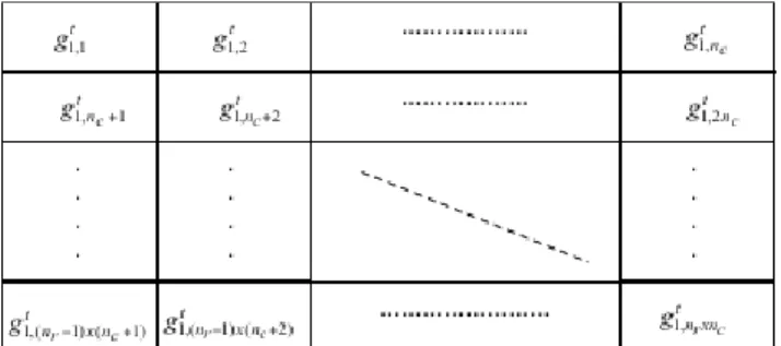
t n m t m t m t m t n t t t t n t t t t m t t t g g g g g g g g g g g g , 3 , 2 , 1 , , 2 3 , 2 2 , 2 1 , 2 , 1 3 , 1 2 , 1 1 , 1 2 1                   g g g I (1)

In this formula , _It _{is the vector of the t}th

generation. g is an individual which consists of genes g. m is the number of individuals in every generation and can be chosen arbitrarily but must be even. If m is not large enough, error cannot be minimized sufficiently. n is the number of genes and can be computed as n = nr x nc.

In the first generation, values of the genes are randomly chosen as zero or . Then, each individual is mapped to cross-section as in Figure 1.

The anomaly of the cross-section for the first individual at position z on the ground is computed as below considering prismatic anomaly model [17],

A1(z)= 2 h=0 nc-1 å x=0 nr-1 å ´6.67´10-8_´Dr_{´{(x´wdt-z´wdt)ln} (h´dpt+dpt)2₊ (x´wdt-z´wdt)2 (h* dpt)2₊ (x´wdt-z´wdt)2 æ è çç ö_ø÷÷-((x´wdt-z´wdt)-wdt)ln (h´dpt+dpt)2₊ ((x´wdt-z´wdt)-wdt)2 (h´dpt)2₊ ((x´wdt-z´wdt)-wdt)2 æ è çç ö_ø÷÷+(h´dpt+dpt)(arctan x´wdt-z´wdt h* dpt+dpt æ è ç ö ø ÷-arctan x´wdt-z´wdt-wdt h* dpt+dpt æ è ç ö ø ÷-h´dpt(arctan x´wdt-z´wdt h* dpt æ è ç ö ø ÷-arctan x´wdt-z´wdt-wdt h* dpt æ è ç ö ø ÷} (2)

All the anomalies of points z from 0 to nc-1, A(z), are

computed and compared with the original anomaly. wdt and

dpt are width and depth of each unit. x and h are column and

row indexes of the units in cross-section. Mean Error (ME) of the individual is designated as the weight function. Ascending sort is applied to all individuals according to their MEs and some of them at the bottom are dismissed after this sort. The number of worst individuals is determined by a rule of keeping the value below the half of the number of individuals. The worst individuals are replaced with the best ones, which are at the top of the list. These individuals, which are obtained after this step, are called chosen individuals.

Before creating the new generation, mutation is applied to the chosen individuals. In this process, some genes are changed with probability of mutation. The value of these genes is turned to (the contrast of the model) if it is 0 or

turned to 0 if it is . Thus, generations can pass local minimums and continues for global minimum of weight function.

To avoid having the same individuals for next generations, location of the individuals in (1) are changed, which is called interleaving. Then, new generation is obtained by using crossover technique. Every two sequential individuals are separated into two parts and the

separation point is chosen randomly for each pair as shown in below for the first pair.

t n t t t t t t t _{g g g g g g g} , 1 6 , 1 5 , 1 4 , 1 3 , 1 2 , 1 1 , 1 1  g (3) t n t t t t t t t _{g g g g g g g} , 2 6 , 2 5 , 2 4 , 2 3 , 2 2 , 2 1 , 2 2  g (4)

Then these two individuals are crossed-over as shown in (5) and (6). (5) t n t t t t t t t _{g g g g g g g} , 1 6 , 1 5 , 1 4 , 2 3 , 2 2 , 2 1 , 2 2  g (6)

After these steps, cross-sections of the individuals indicated may not have a block structure. Thus, units with a density difference in the cross-section, which don’t have any neighbor units with a density difference , are set to zero. Then, whole process is repeated until the global minimum or sufficient error minimization is reached. It is given two synthetic examples; the first one is U type and the other one is a basin model. Based on the anomalies with acceptable errors, GA finds the models satisfactory. Mean Errors (MEs) of these two synthetic modes are 0.087 mGal and 0.073 mGal respectively.

5. Method Application and Results

5.1. Synthetic Data 1

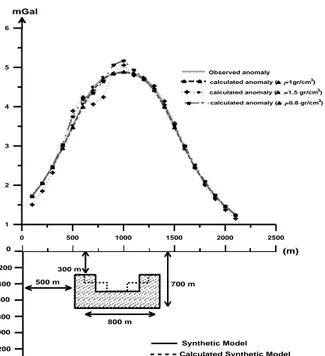
In the first synthetic data, it is used U type model, which is shown in Figure 2. The width and the depth of each unit is 100m and the density difference is 1 gr/cm3. The anomaly of this model is calculated with the prismatic model formulation, which is given in equation 2. Figure 2 shows the anomaly curve of the model.

In genetic algorithm, the purpose is to find a model, in which its anomaly closes to the observed anomaly, given in Figure 2. The first parameter of the genetic algorithm is the number of individuals in one generation and it is chosen as 160. There are 210 genes in each individual. This value is the number of units in the cross-section. The second parameter is the number of individuals, which have worst errors, and it is chosen as 16. These individuals are replaced with the best 16 ones. The last parameter is the ratio of mutation. In our experiments 0.3% seems to be the best value for mutation.

At the end of the 125th generation, it is interrupted the process, because the error of the system has become quite constant. The best individual is shown in Figure 2 with dashed lines. Its anomaly and observed anomaly are given in Figure 2. It is not easy to distinguish these two anomalies, because the anomaly of the model, obtained from genetic algorithm, fits the target anomaly exactly. Mean error is only 0.087 mGal.

Figure 2. First synthetic model: Observed and calculated cross

sections (width and depth of each unit is 100 meters and =1

gr/cm3) and their related underground models. Observed cross-section is indicated with solid line and its structure is given with hatched area. For =1.5 gr/cm3, calculated cross section is shown with (+) symbol. For =0.8 gr/cm3, calculated cross section is shown with ( ) symbol. For =1 gr/cm3, calculated cross section is shown with ( ) symbol and its model is given with dashed lines in cross-section.

5.2. Synthetic Data 2

In the second synthetic data, we consider a basin model, which is given in Figure 3. The width and the depth of each unit is 100m and the density difference is 2 gr/cm3. The anomaly of this model is calculated with the prismatic model formulation, which is given in equation 2. Figure 3 shows the observed anomaly curve of the basin model. There are 320 individuals in each generation and 210 genes in each individual. The number of worst individuals, which are replaced with the best ones, is chosen as 32. Lastly, ratio of mutation is kept constant at 0.3%.

At the end of the 182th generation, the model with dashed lines in Figure 3 is reached. Its anomaly and observed anomaly are shown in Figure 3. It can be said that these are exactly the same, because mean error is 0.073 mGal. Synthetic model and calculated model are very close to each other. There are only two different units, which are at the bottom of the model.

Figure 3. Second Synthetic Model: Observed and calculated

(Segmented Genetic Algorithm) cross sections (width and depth of each unit is 100 meters and =2 gr/cm3) and their related underground models. Observed anomaly is given with solid line and its structure is given with hatched area in the cross-section.

For =2.5 gr/cm3, calculated anomaly is shown with ( )

symbol. For =1.8 gr/cm3, calculated anomaly is shown with ( ) symbol. For =2 gr/cm3, calculated anomaly is shown with (□) symbol and its structure is given with dashed line in the cross-section.

5.3. Real Data 1

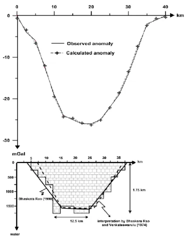
In Figure 4. Godavari Vally, which is used in [1] and [2], is modeled using GA. Depth and the widths of each prismatic piece are 250m and 2.5km respectively. In [1] and [2] is used as -0.4g/cm3. Therefore, it is also used the same value for to compare the models. The anomaly of the model is very close to the observed one and ME is 0.43 mGal. The lower depth of the model is 1.75 km. The average upper and lower widths are 32.5km and 12.5km respectively. (m) 0 200 400 600 800 1000 1200 500 m 800 m 700 m 300 m depth (m) Synthetic Model Calculated Synthetic Model

Observed anomaly calculated anomaly ( =1gr/cm )3 calculated anomaly ( =1.5 gr/cm ) calculated anomaly ( =0.8 gr/cm ) 0 500 1000 1500 2000 2500 1 2 3 4 5 6 3 3 mGal (m) 0 200 400 600 800 1000 500 m 1100 m 700 m 100 m depth (m) Synthetic Model Calculated Synthetic Model

0 500 1000 1500 2000 2500 0 5 10 15 20 25 mGal Observed anomaly calculated anomaly ( =2 gr/cm )3 calculated anomaly ( =1.8 gr/cm )3 calculated anomaly ( =2.5 gr/cm )3

Figure 4. Gravity anomaly profile over the lower Godavari Vally

and its models. Observed anomaly is shown with solid line. Calculated anomaly using SGA is shown with (+) symbol (width is 2.5km and depth is 250m and =-0.4 gr/cm3). SGA model is given with hatched area. Bhaskara Rao and Venkateswarulu (1974) model is given with dashed lines in cross-section. Bhaskara Rao (1990) model is given with solid line in cross-section.

5.4. Real Data 2

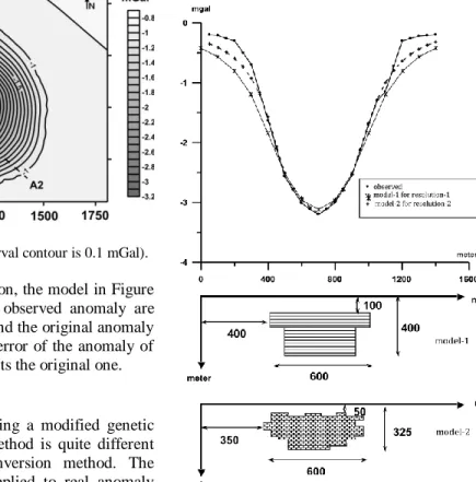
As an application field, anomaly map placed at the Northwest side of the mine ore in Sivas-Gürün in Turkey is chosen (Figure 5). It is assumed that the reason of the anomaly can be the basin, which has –0.5 gr/cm3 density difference according to the crystallized limestone. At the end of the studies on this field, it is found out that the oldest units are the limestone the age of Upper Cretaceous Cenomanien. Upper side of this part, Conglomerate at the age of Neogene, red clay and sandstone are placed as a discordant. The region has faults with direction of NE-SW [17].

After two synthetic examples, real data is selected on the Bouguer anomaly map of Sivas basin, which is shown in Figure 6. Anomalies are measured every 50m and is known as -0.5 gr/cm3 because of the geology. Low pass filter with a 0.02 cutoff frequency is applied to the anomaly map and this residual anomaly map is shown in Figure 7. Profile A1-A2 in residual anomaly map is considered for modeling with genetic algorithm. The width of the units is 50m. To find more precise result by genetic algorithm, the depth of each unit is taken as 25m. There are 832

individuals in each generation and 416 genes in each individual. The number of worst individuals is chosen as 41 and the ratio of mutation is chosen as 0.3% again.

Figure 5. Modified geology map of our working region [18].

Figure 6. Bouguer anomaly map of Sivas-Turkey (interval contour

Figure 7. Residual anomaly map (interval contour is 0.1 mGal).

At the end of the 1000th generation, the model in Figure 8 is reached and, Its anomaly and observed anomaly are shown. The anomaly of our model and the original anomaly are very close to each other. Mean error of the anomaly of our model is only 0.17 mGal and it fits the original one.

6. Conclusion

A new modeling technique using a modified genetic algorithm is very common. This method is quite different and flexible than conventional inversion method. The proposed modeling technique is applied to real anomaly data after having good results with synthetic ones. As a field application, firstly, gravity anomaly of Godavari Vally is used and the model is compared to the references. Secondly, gravity anomaly of carsick basin near Sivas-Gürün in Turkey is considered. Difference of anomaly in the field is computed as -0.5 gr/cm3. Cross-section, which is taken from A1-A2 profile in Figure 7 Bouguer anomaly map, is indicated with a solid line in Figure 8.

The anomaly of the model, which is created by GA, is shown in Figure 8 with dotted line. Both two anomalies are fit satisfactorily. This modeling technique is so powerful that it can be applied to any type of structure without any prior information.

7. Steps of the methods

1. Dividing the cross-section into nr x nc units

2. Generating an initial population for GA

3. Mapping each individual in the population to the cross-section

4. Setting units to zero whose neighbors are all zero 5. Computing the weight function

6. If the anomaly of any individual is close enough to the desired one then STOP THE PROCESS 7. Sorting individuals (worst individuals are replaced with the best ones)

8. Applying mutation

9. Interleaving the individuals (scrambling) 10. Creating the next generation using crossover

technique and GO TO STEP 3.

Figure 8. Observed and calculated anomalies and the models.

Observed anomaly is shown in (.) and calculated anomalies are shown in ( ) and (+) signs.

8. Acknowledgement

This research was supported by Research Institute of Istanbul University (The Project Number: 35156) The authors wish to thank MTA for providing of potential field data for this study.

9. References

[1] Bhaskara Rao, D. (1990), Analysis Of Gravity Anomalies Of

Sedimentary Basins By An Asymmetrical Trapezoidal Model With Quadratic Density Function. Geophysics 55, 226-231.

[2] Bhaskara Rao, V. And Venkateswarulu, P.D. (1974), A

Simple Method Of Interpreting Gravity Anomalies Over

Sedimentary Basins. Geophysical Research Letters 12,

177-182.

[3] Cavicchio, D.J. (1970), Adaptive Search Using Simulated

Evolution. Ph.D. University Of Michigan.

[4] Davis, L. (1987), Genetic Algorithms And Simulated

Annealing. Morgan Kaufmann Publishers, Inc.

[5] Davis, L. (1991), Handbook On Genetic Algorithms. Van Nostrand Reinhold, New York.

[6] Goldberg, D.E. (1989), Genetic Algorithms In Search,

Optimization, And Machine Learning. Addison-Wesley

Publish Co., Inc.

[7] Buckles, B.P. And Petry, F.E. (1992), Genetic Algorithms. Ieee Computer Society Press Technical Series.

[8] Wright, A.H. 1991. Genetic Algorithms For Real Parameteer

Algorithms.

[9] Stoffa, P.L. And Sen, M.K. 1991. Nonlinear Multiparameter

Optimization Using Genetic Algorithms. Inversion Of Plane-Wave Seismograms, Geophysics 56, 1794-1810.

[10] Jin, S. And Madariaga, R. (1993), Background Velocity

Inversion With A Genetic Algorithm. Geophysical Research

Letters, 20, 93-969.

[11] Billing, S., Kennett, B. And Sambridge, M. (1994),

Hypocentre Location: Genetic Algorithms Incorporating

Problem Specific Information, Geophysical Journal

International 118, 693-706.

[12] Boschetti, F., Dentith, M. And List, R. (1995), A Staged

Genetic Algorithm For Tomographic Inversion Of Seismic Refraction Data, Exploration Geophysics 25, 173-178.

[13] Boschetti, F. (1995), Application Of Genetic Algorithms To

The Inversion Of Geophysical Data, Ph.D. Thesis In

Mathematical Geophysics, University Of Western Australia. [14] Boschetti, F., Dentith, M. And List, R. (1996), Inversion Of

Seismic Refraction Data Using Genetic Algorithms,

Geophysics 61, 1715-1727.

[15] Ucan, O.N., Bilgili, E. And Albora, A.M. 2002. Magnetic

Anomaly Separation Using Genetic Cellular Neural

Networks, Journal Of The Balkan Geophysical Society 3,

65-70.

[16] Hall, J.M. (2004), Anovel, Real-Valued Genetic Algorithm

For Optimizing Radar Absorbing Materials, Nasa Project

No: Nasa/Cr-2004-212669.

[17] Telford, W.M., Geldart, L.P., Sheriff, R.E. And Keys, D.A. 1981. Applied Geophysics. Cambridge University Preess, Cambridge.

[18] Albora, A.M. (1992), Study Of Gravity Effect Of Different

Geometrical Structure With Nomograms. Istanbul

University, Institute Of Science And Technology, Msc. Thesis.

Onur Osman was born in Istanbul,

Turkey on September, 1973. He graduated from Electrical Engineering Department of Istanbul Technical University in 1994. Then he received M.Sc. degree from Electrical Engineering in 1998. He received Ph.D. degree from Electrical & Electronics Engineering Department of Istanbul University. He is with Istanbul Arel University in Electrical and Electronics Engineering as Assoc. Prof. His research area is channel coding, modulation, MIMO systems, signal processing on EEG and EMG applications, image processing on MR and CT applications, feature extraction and selection, machine learning, classification and clustering.

Ali Muhittin ALBORA received the BS, MS

and PhD degrees in geophysics engineering from Istanbul University in Istanbul, Turkey, in 1985, 1992 and 1998. He was appointed and assistant professor in 20001, and an associate professor in 2003. since 2003, he has been with Istanbul University, Enginering Faculty department of the Applied Geophysics. His research interests include the the use of potential field methods in the solution of regional and crustal geological problems, and the applications of computer tecniques in geophysics.