The relationship between velocity and interest rate in the cash in advance model

(1)

THE RELATIONSHIP BETWEEN VELOCITY AND INTEREST RATE IN THE CASH IN ADVANCE MODEL

A Master‟s Thesis by SEZĠN SARAÇOĞULLARI Department of Economics Bilkent University Ankara June 2010

S E Z İN S AR AÇ OĞ ULL AR I VEL OCIT Y A ND INTE RES T RA T E B il k en t 201 0

(2)

(3)

(4)

The Institute of Economics and Social Sciences of

Bilkent University

by

Sezin Saraçoğulları

In Partial Fulfilment of the Requirements for the Degree of MASTER OF ARTS

in

THE DEPARTMENT OF ECONOMICS BĠLKENT UNIVERSITY

ANKARA June 2010

(5)

I certify that I have read this thesis and have found that it is fully adequate, in scope and in quality, as a thesis for the degree of Master of Arts in Economics.

--- Dr. Neil Arnwine Supervisor

--- Assoc. Prof. Fatma TaĢkın Examining Committee Member

---

Assoc. Prof. Laurence Barker Examining Committee Member

Approval of the Institute of Economics and Social Sciences

--- Prof. Erdal Erel Director

(6)

iii ABSTRACT

Saraçoğulları, Sezin M.A., Department of Economics

Supervisor: Dr. Neil Arnwine

June 2010

This thesis considers the long run relationship between velocity of money and nominal interest rate with the proposed Cash in Advance model. In the long run analysis, the steady state relationship between velocity and interest rate in CIA model is modeled as a regression. The regression results by using level data are found to be spurious which is caused by non-stationary series. In order to solve this problem, the first differences of the variables are used in the regression. When the drawbacks of using the first differences are taken into consideration, Fully Modified OLS is preferred as the estimation method to find the long run relationship. According to the estimation results, the welfare cost of inflation is found.

Keywords: velocity of money, Cash-in-Advance Model, Fully Modified OLS method

(7)

iv ÖZET

NAKĠT PARA MODELĠNDE PARA DOLAġIM HIZI VE FAĠZĠN ĠLĠġKĠSĠ Saraçoğulları, Sezin

Yüksek Lisans, Ekonomi Bölümü Tez Yöneticisi: Dr. Neil Arnwine

Haziran 2010

Bu çalıĢma, para dolaĢım hızı ve nominal faiz arasındaki uzun dönem iliĢkiyi, önerilen Nakit Para modeli çerçevesinde incelemektedir. Uzun dönem analizinde, Nakit Para modelinde denge durumunda bulunan para dolaĢım hızı ve faiz arasındaki iliĢki regresyon olarak modellenmiĢtir. Tahmin edilen model, zaman serilerinin durağan olmamasından dolayı, sahte regresyon olarak bulunmuĢtur. Bu problemi çözmek için, verilerin birinci farkı alınarak regresyon katsayıları tahmin edilmiĢtir. Birinci fark almanın dezavantajları göz önünde bulundurulduğunda, „Fully Modified OLS‟ metodu kullanılarak regresyon sonuçları tahmin edilmiĢtir. Bu regresyon sonuçlarına göre enflasyonun refah maliyeti hesaplanmıĢtır.

Anahtar Kelimeler: Paranın dolaĢım hızı, Nakit Para modeli, „Fully Modified OLS‟ metodu

(8)

v

ACKNOWLEDGMENTS

I would like to thank Dr. Neil Arnwine for his supervision and guidance through the development of this thesis. I would also like to thank to Assoc. Prof. Fatma TaĢkın, Assoc. Prof. Laurence Barker for their invaluable suggestions. Finally, I want to thank my family and friends AyĢegül Dinççağ and GülĢah Aksu for their support.

(9)

vi TABLE OF CONTENTS ABSTRACT ... iii ÖZET ... iv ACKNOWLEDGMENTS ...v TABLE OF CONTENTS ... vi

LIST OF TABLES... vii

LIST OF FIGURES... viii

CHAPTER I: INTRODUCTION ... 1

CHAPTER II: VELOCITY AND INTEREST RATE IN CASH IN ADVANCE MODEL ... 5

2.1 Literature Review ... 5

2.2 Cash in Advance Model... 10

2.3 Empirical Analysis for the Long Run Relationship... 13

2.3.1 Estimating the Long Run Relationship Using Fully Modified Ordinary Least Squares ... 22

2.3.2 Tests for Parameter Instability ... 28

2.4 Welfare Cost Analysis ... 32

CHAPTER III: CONCLUSION ... 37

SELECTED BIBLIOGRAPHY ... 39

(10)

vii

LIST OF TABLES

1. ADF unit root test results ... 15

2. PP unit root test results ... 16

3. KPSS unit root test results ... 17

4. Regression Results (in the calculation of V, M1 is used) ... 18

5. Regression Results (in the calculation of V, M2 is used) ... 18

6. Regression Results considering first difference of series-1... 19

7. Regression Results considering first difference of series-2... 20

8. Breusch-Godfrey Serial Correlation LM test for Table 7... 22

9. Parameter Stability Tests for Equation 32... 30

(11)

viii

LIST OF FIGURES

1. Logn1 Series between dates 1959 and 2008... 14

2. Logn2 Series between dates 1959 and 2008... 14

3. The Estimated Money Demand Function for 1959, 1981 and 2008 .. 33 4. Actual and Predicted M/GDP versus interest rate ... 33 5. Estimated Welfare Cost of Inflation between years 1959 and 2008... 35 6. Estimated Welfare Cost Function for 1959, 1981 and 2008 ... 36

(12)

1

CHAPTER 1 INTRODUCTION

There are both empirical and theoretical studies that analyze the relationship between the income velocity of money and interest rate i.e. Baumol (1956), Lantane (1954), Kraft A. and Kraft J. (1976) and Lucas and Stokey (1987). In addition to these studies, Cash in Advance (CIA) model by Arnwine (2010) derives a long run relationship between velocity and interest rate. By this motivation, in my thesis, I will investigate the long run relationship between velocity of money and nominal interest rate defined in CIA model by Arnwine (2010) empirically.

Arnwine (2010) presents an axiomatic approach for studying monetary economics. One implication of the study is the need for a „transactions production function‟ in a CIA model. It is the first model that can match the first moment of velocity for any measure of money and frequency of data. The traditional Cash in Advance Model identifies the relationship of interest rate and velocity such that velocity of money depends on interest rate e.g. Lucas and Stokey (1987). Moreover, Lucas and Stokey find that there is a positive relationship between interest rate and velocity. Also, the empirical studies such as Kraft A. and Kraft J. (1976) show that there is one-way causality that flows from interest rate to

(13)

2

velocity. In Cash in Advance by Arnwine (2010), the steady state relation between velocity and interest rate is derived as an equation. In my empirical analysis, I model this relation as a regression by taking the logarithm of the variables. I first test the stationarity of variables since the macroeconomic time series data are usually non stationary. I use Augmented Dickey-Fuller (ADF), Phillips-Perron and the Kwiatkowski Phillips Schmidt Shin (KPSS) unit root tests. The tests indicate that all of the series appear to be integrated of order one.

In the regression model, I include time trend as an explanatory variable besides interest rate. As it is observed from the data, velocity of money is increasing over time. Thus, time trend is important in explaining the velocity of money. When I run the regressions with this specification by using level data, the results show that the regressions can be spurious caused by non-stationary I(1) series. In order to solve this problem, I use the first difference of the series in the regression. The results for the differenced velocity (M2 is used as money aggregate for finding the velocity series) and the interest rate series can be considered as the long run relationship between the variables since estimated coefficient of interest rate is significant, Durbin Watson test indicate „no autocorrelation‟.

There are some complications of using differenced series. Firstly, „differencing the series‟ results in loss of some valuable long-run information. Secondly, the regression results only show the long run relationship between the growth rates of velocity and interest rate which is not the main aim of the analysis. Moreover, level data enables us for the welfare cost analysis with the estimated coefficients found from regression of velocity and interest rate. Thus, I use fully

(14)

3

modified OLS method by Phillips and Hansen (1990) in this study. The method suggests a non-parametric correction for the bias introduced by I(1) regressors in the static regression. Moreover, the method enables to analyse general models with stochastic and deterministic trends (Hansen, 1992). In the first of these structural estimations, I include only the constant term to acquire the long run relationship in the CIA Model. The results show that velocity and interest rate has a negative relationship, which is counter-intuitive and contradicts with the findings of Baumol (1956) and Lucas and Stokey (1987). In addition to this, the coefficients of equations are insignificant. However, when a constant term and time trend are included in the regression, the relationship between velocity, (M1 is used as money aggregate for finding the velocity series) and the interest rate is found to be positive and all the estimated coefficients are statistically significant. Thus, the result is in line with both theoretical and empirical expectations.

Hansen (1992) suggests parameter stability tests for the regressions with I(1) processes. The results revealed that the parameters estimated with FM-OLS are stable in all equations, supporting the validity of the structural regressions. As a result, the cointegrating vector is found for the long run relation between the variables by FM-OLS method. The empirical analysis show that there is a mismatch between the model and the data since the trend growth is significant in the regression model. Hence, the results are important in this analysis because the trend growth has not been studied in this context before in the literature.

Estimating the welfare cost of inflation is crucial especially, if we think of the prevalence of inflation in the world‟s economies. In order to estimate welfare cost, the specification of money demand function is necessary. In this thesis, by

(15)

4

the use of estimated relationship velocity and interest rate, I find the money demand function. According to the estimated money demand function, I calculate the excess burden on social welfare. When the estimated welfare cost in 1959 and 2008 is compared, the welfare cost in 2008 is found to be less than 1959. The results show that trend component pulls down the excess burden. Hence, the importance of time trend for modeling the relationship between velocity and interest rate is understood once more.

I begin by presenting the literature review for CIA models in Chapter 2. I explain CIA Model proposed by Arnwine (2010) in detail since the empirical analysis is based on this model. Then, I analyze the long run relationship between velocity and interest rate empirically. In the last section, welfare cost analysis is presented. Finally, in Chapter 3, I evaluate the results that I found.

(16)

5

CHAPTER 2 VELOCITY AND INTEREST RATE IN THE CASH IN

ADVANCE MODEL

2.1 Literature Review

The CIA literature starts with Clower (1967), Lucas (1980), Swensson (1985), Lucas and Stokey (1987) that is motivated by the question: „why do consumers need to hold money?‟. Cash in Advance model is one of the approaches for justifying why there is demand for money so that the impact of the existence of money on the economy can be analyzed. The main assumption of the model is: „consumers purchase goods in cash that was previously obtained‟. By this assumption, money demand can be explained by consumers‟ need for purchasing some goods.

In the simplest CIA model, the risk free model introduced by Lucas (1980), the representative consumer chooses money balances, consumption and savings subject to the cash in advance constraint Pt ct ≤ mt after observing the state of the world. Consumers hold money only for consumption so that the constraint,

Ptct = mt, will be binding in the risk-free version of this model. The important

aspect of the model is that other assets, say bonds earn a positive interest rate where as holding assets in money has no nominal return. Thus, the real return is negative because of inflation. The result of the simple CIA model is: „velocity of

(17)

6

money is equal to one which is a constant‟. If the Quantity Theory of Money i.e.

MV= PY where M is the money supply, V is velocity of money; P is the price

level and Y represents output in the economy is considered with the CIA constraint that is binding and output is equal to the consumption i.e. Yt = ct , we can easily find this result. However, in the presence of risk, velocity varies below one since CIA constraint does not bind because of the unexpected positive money supply shock.

In our classical view of money, e.g. Baumol(1956) velocity depends on interest rate. This dependence can be found from money demand that is proportional, rather than a constant fraction, to the nominal GDP from Quantity Theory of Money. It is also known that money demand depends on the nominal interest rate negatively. This implies that velocity and nominal interest rate has a positive relationship.

Svensson (1985) adds risk by assuming that the representative consumer chooses consumption, money balances and savings before observing the state of the world. This assumption of Svensson's model differs from the risk free model and changes the results of the model mentioned above. Lucas (1980) also has a version of the model with risk. However, Svensson‟s CIA binds more when money growth is unexpectedly high. In this model, agents want to hold more precautionary balances in case they are in the good state of the world so as to consume more. The constraint becomes Pt ct < mt because of this uncertainty.

Moreover, there is a negative relationship between holding precautionary balances and interest rate. When the interest rate is high, the precautionary balances will be less. Thus, the paper concludes that velocity of money will change as a result of

(18)

7

the uncertainty and also, it will depend on the interest rate.

Lucas and Stokey (1987) introduces cash-credit goods model in which agents consume goods c1 and c2 where c1 must be purchased with cash and c2 is

purchased with credit. Agents choose m, money, before they observe the state of the world. Then, they purchase cash and credit goods c1 and c2 according to the

state of the world. The result of the model showed that velocity of money is not constant. It varies through time. When the interest rate is high enough, agents will purchase c1 less since they will hold their money in bank to gain interest rate but

they will purchase c2 more. Thus, velocity of money i.e. will have a positive

relationship between interest rate.

Hodrick, Kocherlakota and D. Lucas (1991) considered whether the Cash in Advance models generate reasonable patterns for the money holdings. They found that basic Cash in Advance models can not generate enough variation for velocity of money. The results of the paper showed that the overall performance of the cash model is poor. They examined the unconditional moments including the coefficient of variation of velocity and the correlations of velocity with money growth, output growth and the nominal interest rate. They also examined the means and standard deviations of real and nominal interest rates, inflation and real balance growth; they calculated the correlations of inflation with money growth, consumption growth and nominal interest rate. In all, they considered fifteen statistics. For twelve out of fifteen, sample value falls outside of the range determined by predictions of the cash model. For the cash credit model, model fails to reproduce ten out of fifteen statistics. When the cash credit model compared to cash model, they found that credit good generate variation in velocity

(19)

8

for some of the parameter values. Another result of the paper is: in order to generate plausible values of velocity, it is indicated that we have to assume high levels of risk aversion. However, while capturing the variability of velocity, model fails to find low actual interest rate level. When the results of annual and quarterly data are compared, it is revealed that both cash and cash credit model gives poor results with quarterly data. Hence, it turns out to be data frequency matters in research so this concept is addressed in Arnwine (2010). In addition to this, Giovannini and Labadie (1991) also found that the basic Cash in Advance Models are not good at generating plausible asset price and interest rate data. Thus, it generates equity premium puzzle.

There were plenty of empirical studies about the relationship between interest rate and velocity in the early literature. Lantane (1954) tried to examine the relationship between cash balances and interest rates. Then, Lantane (1960) investigated the relation between income velocity and interest rates and conclude that higher interest rate is related to speed up in the turnover money. He indicated that the direction of the causation flows from interest rate to the size of cash balances in proportion to income. However, he pointed out regardless of the direction of the causation, the correlation is high. Mason (1974) used a macroeconometric model to extract the causal movements in the velocity of circulation. He identified a significant statistical relationship between velocity and interest rate but he did not identify the direction of causality. Sims (1972) developed a test for unidirectional causality that he used to determine causality between money and GNP for U.S. postwar period. Kraft A. and Kraft J. (1976) found that there is statistically significant relationship between interest rate and

(20)

9

velocity like Lantane (1960) and Mason (1974). Moreover, he found that there is a unidirectional causality flowing from interest rate to velocity.

In this thesis, my purpose is to understand the relationship between interest rate and velocity and find an econometric model that is consistent with the literature and Cash in Advance model proposed by Arnwine (2010). In order to accomplish this, I will investigate the „cointegration‟ between the variables to find the long run relation. In literature, the concept of „cointegration‟ is introduced by Granger (1981). Afterwards, Engel and Granger (1987) provided a firm theoretical base for representation, testing, estimating and modelling of cointegrated nonstationary time series data. Afterwards, some of the studies add dynamic components that are either differences or lags for estimating alternative cointegrating regressions i.e. Charemza and Deadman (1992), Cuthbertson et al. (1992), Inder (1993), Phillips and Loretan (1991), Saikkonen (1991). Other studies focus on with the corrections and modifications to the static parameter estimates ie. Engle and Yoo (1991), Park and Phillips (1988), Phillips and Hansen (1990). In this study, fully modified OLS proposed by Phillips and Hansen (1990) is used since the method advocates the use of some corrections to the OLS estimator to eliminate bias. Moreover, the tests proposed by Hansen (1992) are conducted to show that whether the parameters are stable in the estimated regression. By this way, I find the long run relationship between the variables empirically and compare the relationship with the theoretical model. In Section 2.2, I lay out the theoretical model.

(21)

10

2.2 Cash in Advance Model

Arnwine (2010) introduced an Impossibility Theorem for CIA models to satisfy axioms governing the behaviour of modelling. It is stressed that the unit free measures within a monetary model should not vary with the unit of monetary account or with the frequency of analysis in the steady state equilibrium. The CIA model proposed is a time-dynamic and general equilibrium extension of Baumol's (1952) model.

The shoe leather or income share denoted by s is the proportion of income used up conducting financial transactions. The resource constraint of the shoe leather is the following:

where ct is consumption and yt is output. The nominal CIA constraint is given

below:

The left hand side of the equation is the sum of consumption and shoe leather

spending. The right hand side is money stock times the income velocity of money which is a function of the shoe leather or income share, st. Consumer‟s budget

constraint that is in real terms is the following equation:

In the equation, is and the inflation rate is . Nominal money supply evolves with the process where ω is the gross money growth rate. In addition to this, output evolves with the process:

(22)

11 following value function:

Consumer maximizes the value function subject to the constraints (2) and (3). The first order conditions are shown below where λ and μ are the Lagrange multipliers of the budget and CIA constraint respectively:

and the envelope theorem is:

If we plug Equation (7) to Equation (8) we will have:

Now, λ can be found from Equation (5) and Equation (6). Thus, it will be:

where is the derivative of the velocity production function with respect to s and nt is the velocity at time t. The Lagrange multiplier μ can also found from

Equation (5) and Equation (10) as the following:

When Equation (10) and Equation (11) are plugged into Equation (9) and Fisher‟s relation is considered, we will have:

(23)

12

The above equation links the discounted expected value of the present and future value of marginal consumption ratio with the current interest rate.

The steady state is analyzed with constant output level and constant money growth rate. Time script is omitted for showing the steady state equations so the Euler equations governing the demand for money become as the following:

Combining the two equations, we have a single expression governing the optimal shoe leather expenditure in steady state equilibrium.

The long run relationship between velocity and interest rate is derived and shown below:

where is the constant and σ is the interest elasticity of money demand. In addition to this, the direct transactions production function is found as the following:

The long run relationship derived in the model can be considered by taking logarithm of Equation 16. Then, it can also be written as a regression equation given in below:

(24)

13

Equation (18), the long run relationship between interest rate and velocity should be analyzed empirically. The cointegration between variables needs to be determined. Moreover, the appropriate model should be chosen and the cointegrating vector should be found to conclude such a long run relationship exists between these variables.

2.3 Empirical Analysis for the Long Run Relationship

In this analysis, I preferred annual (1959-2008) U.S. data. The sample data consists of gross domestic product (GDP), monetary aggregate M1, M2 and interest rate (U.S. Government Treasury Bill Rates). M1 consists of notes and coins (currency) in circulation, traveler's checks of non-bank issuers, demand deposits and other checkable deposits (OCDs). M2 consists of the components in M1, savings deposits, time deposits less than $100,000 and money-market deposit accounts for individuals. The velocity is calculated using GDP and monetary aggregate, M1 or M2. Velocity, denoted by n, is found from Quantity Theory of Money so n=PY/M where PY is GDP and M is money stock. For further analysis, I will denote n1 for the velocity when M1 is used as monetary aggregate and n2 for

the velocity when M2 is used as monetary aggregate. The graphs of logn1 and logn2 series are given in Figure 1 and Figure 2. According to the graphs, time

(25)

14

Figure 1: Logn1 Series between dates 1959 and 2008

Figure 2: Logn2 Series between dates 1959 and 2008

1.2 1.4 1.6 1.8 2.0 2.2 2.4 60 65 70 75 80 85 90 95 00 05 LOGN1 .50 .55 .60 .65 .70 .75 .80 60 65 70 75 80 85 90 95 00 05 LOGN2

(26)

15

Macroeconomic time series are generally non-stationary. There are many tests used to determine stationarity of a series. In this thesis, the stationarity of the variables will be tested by using Augmented Dickey-Fuller (ADF), Phillips-Perron and Kwiatkowski Phillips Schmidt Shin (KPSS) unit root tests.

The model suggested for the ADF test is as the following:

where α is a constant and β is the coefficient on the time trend. m is the number of lags in the autoregressive process. For α = 0 and β = 0, the model will be a random walk; whereas for β = 0, the model will be a random walk with drift. The null hypothesis of the test is „series is nonstationary or has a unit root‟ (Ho: γ=0), and alternative hypothesis is „series is stationary‟.

The unit root tests for the velocity of money and interest rate are performed using Eviews-5. The results of the ADF test are shown in Table 1:

ADF Test Statistic Critical Value 1% 5% 10% Logn1 (level) -1.1475 -3.5745 -2.9238 -2.5999 Logn1 (1st difference) -4.0778 -3.5745 -2.9238 -2.5999 Logn2 (level) -1.5791 -3.5745 -2.9238 -2.5999 Logn2 (1st difference) -4.8941 -3.5745 -2.9238 -2.5999 Logi -2.8298 -3.5745 -2.9238 -2.5999 Logi (1st difference) -6.4906 -3.5812 -2.9266 -2.6014

Table 1: ADF unit root test results

(27)

16

with the critical values, we do not reject the null hypothesis which is indicating the presence of unit root for all series. However, for the first differences, we reject the null hypothesis for all the significance levels. Thus, Logn1, Logn2 and Logi are all integrated of order one.

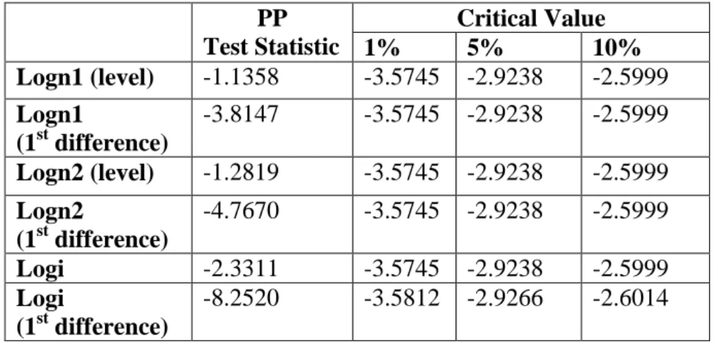
The Phillips–Perron (PP) unit root test allows for the errors that are not iid. The test considers potential serial correlation in the errors by employing a correction factor. The long–run variance of the error process is estimated with a different version of the Newey–West formula. The results of the PP test are in Table 2. The PP unit root results also show that Logn1, Logn2 and Logi are integrated of order one.

PP Test Statistic Critical Value 1% 5% 10% Logn1 (level) -1.1358 -3.5745 -2.9238 -2.5999 Logn1 (1st difference) -3.8147 -3.5745 -2.9238 -2.5999 Logn2 (level) -1.2819 -3.5745 -2.9238 -2.5999 Logn2 (1st difference) -4.7670 -3.5745 -2.9238 -2.5999 Logi -2.3311 -3.5745 -2.9238 -2.5999 Logi (1st difference) -8.2520 -3.5812 -2.9266 -2.6014

Table 2: PP unit root test results

An alternative unit root test is Kwiatkowski, Phillips, Schmidt, Shin (KPSS, 1992) test that has a null hypothesis of stationarity. The unit root test can be conducted under the null hypothesis of either trend or level stationarity. Inference from this test is complementary to the tests that are based on Dickey–

(28)

17

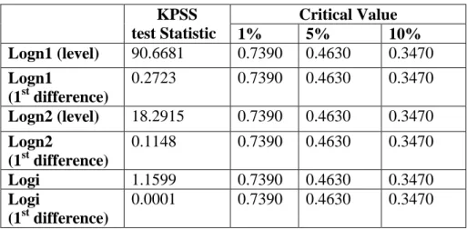
Fuller distribution. The KPSS test is also used together with those tests to investigate whether a series is fractionally integrated or not. The results of the KPSS test are shown in Table 3:

KPSS test Statistic Critical Value 1% 5% 10% Logn1 (level) 90.6681 0.7390 0.4630 0.3470 Logn1 (1st difference) 0.2723 0.7390 0.4630 0.3470 Logn2 (level) 18.2915 0.7390 0.4630 0.3470 Logn2 (1st difference) 0.1148 0.7390 0.4630 0.3470 Logi 1.1599 0.7390 0.4630 0.3470 Logi (1st difference) 0.0001 0.7390 0.4630 0.3470

Table 3: KPSS unit root test results

The KPSS unit root test results show that all the series are integrated of order one. We reject the null hypothesis „series is stationary‟ for all series in level. However, we do not reject the null hypothesis for the first differences of the series.

The unit root tests showed that all series are non-stationary and integrated of order one. Hence, non-stationarity of these series will be a major problem while constructing the long run relationship defined in CIA model. First of all, the long run relationship is investigated by adding trend in the linear regression equation into the model. The following model is estimated by Ordinary Least Squares (OLS) method:

(29)

18

The results of the regression are given in Table 4 and Table 5.

Dependent Variable: LOGN1 Method: Least Squares Sample: 1959 2008 Included observations: 50

Variable Coefficient Std. Error t-Statistic Prob.

C 1.674595 0.069602 24.05956 0.0000

LOGI 0.099836 0.022566 4.424223 0.0001

TIME 0.019122 0.000855 22.35673 0.0000

R-squared 0.914102 Mean dependent var 1.857658

Adjusted R-squared 0.910447 S.D. dependent var 0.287285

S.E. of regression 0.085971 Akaike info criterion -2.011486

Sum squared resid 0.347379 Schwarz criterion -1.896765

Log likelihood 53.28715 F-statistic 250.0812

Durbin-Watson stat 0.260586 Prob(F-statistic) 0.000000

Table 4: Regression Results (in the calculation of V, M1 is used)

Dependent Variable: LOGN2 Method: Least Squares Sample: 1959 2008 Included observations: 50

C 0.532831 0.036253 14.69765 0.0000

LOGI 0.010431 0.011754 0.887449 0.3794

TIME 0.004456 0.000445 10.00186 0.0000

(30)

19

The regression results indicate significant coefficients with α=0.01 significance level except logi in Table 2. R-squared of the regressions are found to be 91 percent and 68 percent respectively that are very high. Overall, the regressions are significant. However, Durbin Watson statistics are 0.26 and 0.27, respectively. The statistics that are calculated from the regressions are not interpretable since the Durbin Watson statistic is low and goodness of fit measures are „too high‟. Thus, the results given in Table 4 and Table 5 may indicate spurious regressions that are caused by non-stationary (trended) velocity and interest rate data.

As all of the series appear to be intergrated of order one, taking the first difference of the series removes the problem of non-stationarity. Then, the model becomes the following when I take the first difference:

The estimation results of the above equation are found in Table 6 and Table 7.

Dependent Variable: DLOGN1 Method: Least Squares Sample (adjusted): 1960 2008

Included observations: 49 after adjustments

C 0.022109 0.005170 4.276382 0.0001

DLOGI 0.034093 0.014088 2.419951 0.0194

(31)

20

Dependent Variable: DLOGN2 Method: Least Squares Sample (adjusted): 1960 2008

Included observations: 49 after adjustments

C 0.002092 0.003134 0.667602 0.5077

DLOGI 0.031329 0.008540 3.668394 0.0006

Table 7: Regression Results considering first difference of the series-2

The regression results show that the coefficients are significant with 0.05 level. However, in Table 7 constant term is found to be insignificant. The goodness of fit is higher when n2 is used in the estimation. Moreover, the

regressions are significant with 0.05 level.

Durbin Watson test is used to detect whether the residuals in the regression are autocorrelated or not. The null hypothesis of the test is no autocorrelation,

and alternative is positive or negative autocorrelation,

where . As is the residual at time t, then the test statistic is:

d=2 indicates no autocorrelation since d is approximately equal to 2(1-r) where r is the autocorrelation of residuals. The values d are between 0 and 4. If the test

(32)

21

statistic is found to be less than 2, there is an evidence of positive autocorrelation. On the other hand if the test statistic is higher than 2, one can say that errors are negatively correlated.

In order to test for positive correlation at significance α, the test statistic d is compared to the lower and upper critical values denoted dL and dU respectively.

If d < dL, there is evidence for positive autocorrelation. If d > dU, there is no

evidence for positive autocorrelation. However, for dL<d< dU, the test is

inconclusive. For negative correlation at significance α, test statistic (4-d) is compared with the critical values. If (4-d) < dL, there is evidence for negative

autocorrelation. If (4-d) > dU, there is no evidence for negative autocorrelation.

For dL<(4-d)< dU, the test is inconclusive. In Table 6 and Table 7, Durbin Watson

statistic is found to be 1.0925 and 1.5049 respectively. The lower and upper critical values are: dL=1.503 and dU=1.585 for the significance level of 0.05. The

error terms of the regression presented in Table 6 exhibits positive autocorrelation since d=1.0925 is lower than dL. However, for the regression in Table 7, Durbin

Watson test is inconclusive since d=1.5049 is between the lower and upper critical values.

Breusch-Godfrey Serial Correlation LM test is conducted for the regression in Table 7 since the Durbin Watson test is inconclusive. The null hypothesis of test is „no serial correlation of any order up to p' ( ). According to the LM test result in Table 8, there is no evidence of serial correlation.

(33)

22

Breusch-Godfrey Serial Correlation LM Test:

F-statistic 1.630456 Probability 0.207196

Obs*R-squared 3.310852 Probability 0.191011

Table 8: Breusch-Godfrey Serial Correlation LM test for Table 7

The regression in Table 7 can be considered as the long run relationship between interest rate and velocity from the above analysis. Hence, if the model is defined as in Equation 21, the fitted equation will be the following:

The above equation gives the relation between the first difference of velocity and interest rate. However, the defined relation in Equation 18 cannot be captured by Equation 22. Moreover, „differencing the series‟ results in loss of some valuable long-run information in the data. Thus, the long run relationship between variables should be estimated by using „cointegration‟ regression. In the following section, the cointegrated relationship is modelled using FM OLS by Phillips and Hansen (1990).

2.3.1 Estimating the long run relationship using Fully Modified

Ordinary Least Squares

The long run relationship between velocity of money and interest rate can be modelled by using fully modified OLS (Hansen, 1992). The main reason for choosing FM OLS is because the method corrects bias in the static regression. The static regression approach is simple and easy to use but it has certain drawbacks.

(34)

23

It ignores dynamics, simultaneity. In addition, it is based on arbitrary normalisation. Even though, OLS estimates are super consistent, they can be biased in finite sample as it is found in the simulation studies. Thus, Phillips and Hansen (1990) have suggested a non-parametric correction for this bias. The corrected OLS regression is called the fully modified OLS. The FM OLS used in this study is extended to cover general models with stochastic and deterministic trends (Hansen, 1992). The cointegration regression model considered in the following way:

where the process is defined by the equations:

The vectors are given below:

where consists of mean zero random vectors that has elements and

has elements. The elements of are defined to be nonnegative integer powers of time in which has elements and has elements. The trends can be placed into the model through and it is also stressed in the paper that constant term can be included in this vector. The trends show the behaviour of the stochastic regressors, . If the stochastic regressors are specified as I(1) with a deterministic trend, in this case equals a constant and a time trend. If and are deterministically cointegrated, the levels regression

(35)

24

only contain a constant. Then, and . If a time trend is needed in the levels regression, and there will not be in the equation. Moreover, when there is no time trend in the model specified,

and there will not be in the equation.

The nuisance parameters given below are used in the formulation of the statistics derived.

The matrices are partitioned that conform to u:

and

Ω is referred as the long run covariance matrix. Moreover, and are defined as the following:

is called the long run variance of conditioned on . is the bias related to the endogeneity of the regressors after the correction. The method of Phillips and Hansen (1990) has two steps in estimation. In the first step the defined covariance parameters, and are estimated. For the estimation, prewhitened kernel estimator with the plug-in bandwidth is used. First of all, Equation (23) is estimated by ordinary least squares, denoting the parameter estimates B and the residuals . Then, Equation (24) is estimated by ordinary least squares in differences. The estimated equation will be

(36)

25

Kernel is used to estimate the covariance matrices Ω and Λ from the residuals, . The kernel estimator will be biased which will increase the variance of the estimator if a large bandwidth parameter is not used. Hence, Hansen (1992) proposes to use an estimator based on prewhitening. The residuals, follow VAR(1) process: . Then, the kernel estimator is used for the whitened residuals The estimators will have the following form:

in the above equations, w(.) is the kernel that gives positive semi-definite estimates and M is a bandwidth parameter. The covariance parameter estimates

are found by recoloring: and

where .

Kernel and bandwidth parameters should be chosen for the estimation. Kernel should give positive semidefinite estimates. Thus, Hansen (1992) recommends Bartlett, Parzen and quadratic spectral (QS) kernels. Moreover, the plug-in bandwidth estimator is set according to paper by Andrews (1991). The choices of bandwidth for Bartlett, Parzen and QS kernels are the following:

In the above equations, and are found from approximating parametric models. Andrews suggests the univariate AR(1) models for each element of . If we denote the autoregressive and innovation variance estimates for the ith element

(37)

26

of as and where i=1,..,p, then we have the following:

There are several advantages of using the plug-in bandwidth parameter as Hansen (1992) pointed out. Determining the bandwidth in advance removes the arbitrariness. Also, the simulation studies of Park and Ogaki (1991) show that using a plug-in bandwidth parameter improves the mean square error of semiparametric estimates of the cointegrating relation.

For the estimation of regression parameters, and that are defined in Equation (27) and Equation (28) are used. The dependent variable is transformed as . Thus, the FM estimator will be the following:

and residuals can be found from the equation: . Note that we have:

(38)

27 The scores meet the condition .

The long run relationship of interest rate and velocity is estimated by using FM OLS so as to correct the bias in the static regression. The results are found with the Matlab code provided by Hansen (1992). The detailed outputs that include standard errors are given in Appendix. In the regression, first of all, only the constant term is included since CIA Model provides such a relationship between the variables in Equation (18). The fitted equations found from FM OLS are the following:

The fitted equations imply that velocity and interest rate have a negative relationship, which contradicts with the theory e.g. Lucas and Stokey (1987). According to theory, as interest rate increases, money demand is expected to decrease where as from Quantity Theory of Money, velocity is expected to increase. So, a positive relationship should exist between velocity and interest rate. Moreover, the coefficients in Equation (32) and Equation (33) are found to be insignificant. Thus, both constant term and trend is included in regression since we observe a trend in the data. The results estimated from FM OLS are given below:

The coefficient of logit is found to be insignificant in Equation (35).

However, all coefficients in Equation (34) are significant and the relationship between velocity and interest rate is found to be positive which is consistent with

(39)

28

the theory as it is explained before. Thus, Equation (34) gives the long run relationship by utilizing FM OLS method. In addition to this, Hansen (1992) proposes tests for parameter stability in regressions with I(1) processes.

2.3.2 Tests for Parameter Instability

Hansen (1992) described the test statistic for parameter stability in FM OLS in cointegrated regression models. In order to consider the possibility of parameter instability the model in Equation (23) modified the coefficient matrix A such that it depends on time:

The null hypothesis of the tests for parameter instability is that the coefficient At is

constant. However, the alternative hypothesis differs. The first two tests proposed by Hansen (1992) consider that At obeys a single structural break at time t, where

1 < t < n:

From the above equations, we can write the null hypothesis as . In the first test, the time when the structural break occurs is known under the alternative hypothesis: . The test statistic for the first test given in Hansen (1992) is the following:

(40)

29 and

In the second test, the time when the structural break occurs is unknown so the alternative hypothesis is set to A1≠A2, [t/n] є τ such that τ is a compact subset of

(0,1) interval. Thus, the test statistic is:

At is modelled as a martingale process: where

in the third and fourth tests. The null hypothesis is set such that the variance of the martingale differences is 0 ( ). The

alternative hypothesis for the third test is where

t/n є τ, the test statistic is:

The alternative hypothesis for the fourth test is

and the test statistic is given by Hansen (1992):

The three tests, SupF, MeanF and Lc, are calculated by Matlab and

according to the test results, I determine whether the estimated models given in Equation 32 to 35 are stable or not. The test statistics and p-values are found for each equation:

(41)

30

Test Statistics P-value*

Lc 0.1792 0.2

MeanF 1.4225 0.2

SupF 3.2991 0.2

*".20" means ">= .20"

Table 9: Parameter Stability Tests for Equation 32

Lc 0.1193 0.2

MeanF 0.9876 0.2

SupF 2.2767 0.2

*".20" means ">= .20"

Table 10: Parameter Stability Tests for Equation 33 Test Statistics P-value*

Lc 0.1849 0.2

MeanF 2.0501 0.2

SupF 4.1248 0.2

*".20" means ">= .20"

<Lc 0.0614 0.2

MeanF 0.7482 0.2

SupF 1.8276 0.2

*".20" means ">= .20"

The p-values for all tests are found to be greater than 0.2. Hence, we do not reject the null hypothesis in all tests for every model. The parameters of the estimated models are stable as a result of Lc, MeanF and SupF tests.

The fitted equation given in (34) is both stable and has significant coefficients. When Equation (34) is compared to Equation (35), the coefficient of logit is found

to be positive. As it is explained before, one reason for finding this result is the significance of the coefficients estimated. Another reason can be from the

(42)

31

definitions of M2 and M1. As M2 has a broader definition for money aggregate, there may be some components of M2 that cannot be explained by interest rate. Thus, in order to show the change in the sign of coefficient logit that is caused by

the components in M2 but not in M1, I take the difference between M2 and M1 and calculate velocity with this difference, denote it by . Then, when I estimate velocity calculated with the differenced M2 and M1 on interest rate and trend by FM OLS, I have the following results:

According to the estimation results, the coefficient of logit is found to be

negative. The components that are savings deposits, time deposits that are less than 100000 dollars and money market deposits in M2 but not in M1 do not give consistent results with the theory; so M1 should be used for finding the velocity series. Hence, from the above reasons, Equation (34) is the estimation result that defines the long run relationship between velocity and interest rate.

In the estimated long run equation, the coefficient of the trend gives the percentage change in velocity with time. According to Equation (34), the coefficient of logit is 0.208 that is interest rate elasticity of velocity. One percent

change in interest rate leads approximately 0.2 percent change in velocity. In addition to this, one unit change in time leads 0.02 percent change in velocity.

As FM estimator is found from Equation (39), the error terms can be found

from the equation: where and the plus

script is used to show the transformed variables. According to this, the goodness of fit measure is calculated and found to be high enough, approximately 76 percent.

(43)

32

The equation that is estimated by FM OLS is preferable when the significance of coefficients and goodness of fit is compared with the other models. Moreover, the estimation results are consistent with the theory. A constant and trend term should be taken into account for modelling the relationship between velocity and interest rate empirically. Hence, the theoretical model presented should also consider the empirical model estimated to construct the relationship between velocity and interest rate.

2.4 Welfare Cost of Inflation

The model in Equation (34) defines the relationship between velocity and interest rate. Then, velocity and has the following relationship:

where . When the estimated coefficients from Equation (34) are plugged into Equation (42), the equation becomes:

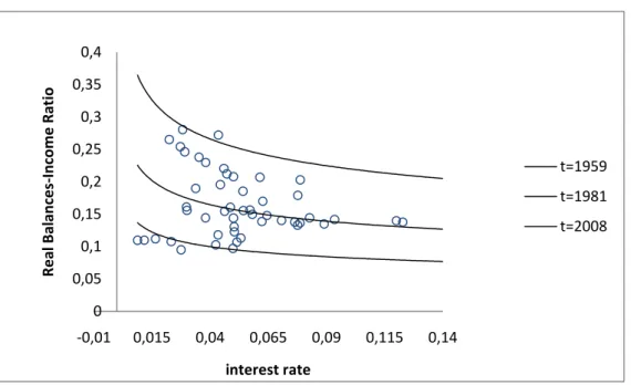
The Quantity Theory of Money implies . Thus, the ratio of M1 to GDP can be found from: so that the real balances takes the form . The money demand is inversely proportional to interest rate. In Figure-3, the estimated demand curve is shown when years are taken 1959, 1983 and 2008 respectively. Moreover, the actual real balances-income ratio is plotted with respect to interest rate.

Figure-4 shows the actual and predicted real balances income ratio with respect to interest rate. The fitted values track the actual real balances-income

(44)

33

ratio successfully. However, predicted series have peaks in some years which are not observed in the actual series. This problem occurs because the interest rate elasticity remains higher to fit the long term trends and prevents a good fit in a year-to-year basis as it is explained by Lucas (2000).

Figure 3-The Estimated Money Demand Function for 1959, 1981 and 2008

Figure 4-Actual and Predicted M/GDP versus interest rate 0 0,05 0,1 0,15 0,2 0,25 0,3 0,35 0,4 -0,01 0,015 0,04 0,065 0,09 0,115 0,14 R e al B al an ce s-In co m e R atio interest rate t=1959 t=1981 t=2008 0,0000 0,0500 0,1000 0,1500 0,2000 0,2500 0,3000 0,3500 0,02 8 0,029 0,047 0,044 0,063 0,093 0,07 9 0,054 0,062 0,057 0,043 0,012 0,050 actual M/GDP predicted M/GDP

(45)

34

According to the above analysis, the excess burden on social welfare can be found from the estimated money function. Bailey (1956) defines welfare cost of inflation as the area under the inverse demand function (the consumer‟s surplus) that is gained by reducing interest rate from i to zero. Suppose is the estimated money demand function and is the inverse function, hence the welfare cost function can be written as below:

The welfare cost for the estimated demand function in Equation (44) can be found as:

The welfare cost of inflation can be calculated for each year with the actual interest rates by considering Equation (46). In Figure 5, the calculated welfare cost for each year is shown. According to this, welfare cost is the lowest in 2003 that is 0.04 percent where as it is found to be the highest in 1981 that is 0.51 percent. Moreover, in Figure 6, the estimated welfare cost function for years 1959, 1981 and 2008 found from the money demand equation is presented.

According to the welfare cost analysis, 3 percent interest rate is taken as a benchmark since it is rate that will arise in the U.S. economy when the inflation rate is nearly zero. Hence, the estimated welfare gain from reducing interest rate to zero levels can be considered. For year 1959, the welfare gain from reducing interest rate 3 percent to 0 is 0.002 fraction of the income. Thus, moving from zero inflation to deflation implies a gain of 0.002 in the welfare. The welfare gain from reducing interest rate 14 percent to 3 is about 0.006. From these results, I can

(46)

35

say that the gain in welfare from moving a positive inflation rate to zero inflation rate is 0.006 fraction of the income. For year 2008, the welfare gain moving from deflation to zero inflation rate is 0.0008. The welfare gain moving from positive inflation to zero inflation is 0.002. If we compare 1959 and 2008 results, the welfare gain in 2008 is less than 1959. The reason of this result is the trend component since it is important in explaining the relationship between velocity and interest rate. Hence, it is also effective for modelling the relationship between money demand and interest rate.

Figure-5 Estimated Welfare Cost of Inflation between years 1959 and 2008 0 0,001 0,002 0,003 0,004 0,005 0,006 1950 1960 1970 1980 1990 2000 2010 2020

welfare cost

(47)

36

Figure-6 Estimated Welfare Cost Function for 1959, 1981 and 2008 0 0,001 0,002 0,003 0,004 0,005 0,006 0,007 0,008 0,009 0 0,05 0,1 0,15 0,2 w e lfar e c o st interest rate t=1959 t=1981 t=2008

(48)

37

CHAPTER 3 CONCLUSION

I investigate the long run relationship between interest rate and velocity using a variation of the Cash in Advance Model introduced by Arnwine (2010) where velocity is a function interest rate in the steady state. In the empirical analysis, the steady state relationship defined by the model is estimated by an OLS regression. However, non-stationarity of the series complicates the analysis. First of all, time trend is included in the regression. The results showed that the regressions are spurious which is caused by the non-stationarity of variables. Thus, first differences of the variables are used in the regressions to prevent this problem. However, taking the first difference of data results in loss of long-run information in the data. Moreover, the model proposes to use the current values of velocity and interest rate.

Based on the analysis, the long run relationship between variables is estimated by using „cointegration‟ regression. It is modelled using FM OLS by Phillips and Hansen (1990). By this way, the bias in the static regression is corrected and appropriate coefficients are found. The results of this method indicate that constant and trend should be included in the regression equation to find the coefficients that are both significant and consistent with the theory. Hence, the empirical model should be considered while constructing the long

(49)

38

run relationship in CIA model by Arnwine (2010).

The welfare cost of inflation for each year is found from the estimated money demand function. The results for 1959 and 2008 are compared and it is found that the welfare gain in 2008 is less than 1959. According to this, it is concluded that the trend component has a significant effect in the relationship between interest rate and money demand.

For future studies, one can build a CIA model that considers technological growth since the trend component is important for specifying the relationship between velocity and interest rate. In addition to this, the short run dynamics of velocity should be considered since it may add to welfare cost of inflation estimated.

(50)

39

SELECTED BIBLIOGRAPHY

Andrews, Donald W.K. 1991. "Exactly Unbiased Estimation of First Order Autoregressive-Unit Root Models," Cowles Foundation Discussion Papers 975, Cowles Foundation, Yale University.

Arnwine, Neil 2010. “Classical Money Demand and Neoclassical Monetary Models”, Economics Department of Bilkent University.

Bailey, Martin J. 1956. “The Welfare Cost of Inflationary Finance” Journal of

Political Economy, 64, 93-110.

Baumol, William 1952. “The Transactions Demand for Cash: An Inventory-theoretic Approach”, Quarterly Journal of Economics, 66: 545-556. Charemza, W.W. and D.F. Deadman 1992. “New Directions in Econometric

Practice”, Edward Elgar, England.

Clower, Robert 1967. " A Reconsideration of the Microfoundations of Monetary Theory ”, Western Economic Journal, December.

Cuthbertson, K., S.G. Hall and M.P. Taylor 1992. “Applied Econometric Techniques”, Phillip Allan, New York.

Engle, R.F. and C.W.J. Granger 1987. “Cointegration and Error Correction: Representation, Estimation and Testing”, Econometrica, 55, 251-76. Engle, R.F. and B.S. Yoo 1991. “Cointegrated Economic Time Series: An

Overview with New Results”, in R.F. Engle and C.W.J Granger (eds.),

Long-run Economic Relationships: Readings in Cointegration, Oxford

University Press, Newyork.

Giovannini, Alberto and Labadie, Pamela 1991. “Asset Prices and Interest Rates in Cash-in-Advance Models”, Journal of Political Economy, 99: 1215-1251.

Granger, C.W.J. 1981. “Some Properties of Time Series Data and Their Use in Econometric Model Specification”, Journal of Econometrics, 16, 121-30.

(51)

40

Hansen, Bruce E. 1992. “Tests for Parameter Instability in Regressions with I(1) Processes”, Journal of Business and Economic Statistics, 10: 321-335.

Hodrick, Robert J., Kocherlakota, Narayana and Lucas, Deborah 1991. “The Variability of Velocity in Cash in Advance Models”, Journal of Political

Economy 99: 358-384.

Inder, B. 1993. “Estimating Long-run Relationships in Economics”, Journal of

Econometrics, 57: 53-68.

Kraft A. and Kraft J. 1976. “ Income Velocity and Interest Rates: A Time Series Test of Causality ”, Journal of Money, Credit and Banking Vol. 8 No. 1, 123-125.

Lantane, H. A. 1954. “Cash Balances and the Interest Rate: A Pragmatic Approach”, Review of Economics and Statistics 34, 456-60.

Lantane, H. A. 1960. “ Income Velocity and Interest Rates: A Pragmatic Approach”, Review of Economics and Statistics 42, 445-49.

Lucas, Robert E.,Jr. 1980. “Equilibrium in a Pure Exchange Economy”, Economic

Inquiry 18: 203-220.

Lucas, Robert E., Jr. 1982. “Interest Rates and Currency Prices in a Two Country Model”, Journal of Monetary Economics.

Lucas, Robert E., Jr. 2000. “Inflation and Welfare”, Econometrica, Vol. 68, No. 2, 247-274.

Lucas, Robert E., Jr. and Stokey, Nancy L. 1987. “Money and Interest in a Cash in Advance Economy”, Econometrica.

Mason, J. M. 1974. “ A Structural Study of the Income Velocity of Circulation”

The Journal of Finance 29, 1077-86

Park, J.Y. and Ogaki, M., 1991. "Inference in Cointegrated Models Using VAR Prewhitening to Estimate Shortrun Dynamics," RCER Working Papers 281, University of Rochester.

Park, J. Y. and P.C.B. Phillips, 1988. “ Statistical Inference in Regressions with Integrated Processes: Part I”, Econometric Theory, 4, 468-97.

Phillips, P.C.B. and B.E. Hansen, 1990. “Statistical Inference in Instrumental Variables Regression with I(1) Processes”, Review of Economic Studies, 57, 99-125.

Phillips, P.C.B. and M. Loretan, 1991. “ Estimating Long-run Economic Equilibria”, Review of Economic Studies, 58, 407-36.

(52)

41

Saikkonen, P. 1991. “Asymptotically Efficient Estimation of Cointegration Regressions, Economic Theory, 7, 1-21.

Sims, C. A. 1972. “Money, Income and Causality”, American Economic Review

62, 540-52.

Svensson, Lars E.O. 1985. “Money and Asset Prices in a Cash in Advance Economy”, Journal of Political Economy.

(53)

42

APPENDIX

Output A1

Fully Modified Regression Results Sample Size 50

Parameters Estimates are listed by row

Standard Errors are to the right of each estimate I(1) variables

-0.838068 0.474312 Constant, Trend, etc -0.677919 1.465007

Method of Estimation of Covariance Parameters: Pre-whitened

Quadratic Spectral kernel

Automatic bandwidth selected: 3.163547 Tests for Parameter stability

Test Statistic P-value (".20" means ">= .20") LC 0.179146 0.200000

MeanF 1.422446 0.200000 SupF 3.299094 0.200000

Output A2

(54)

43 Sample Size 50

-0.183574 0.111480 Constant, Trend, etc 0.057751 0.344328

MeanF 0.987575 0.200000 SupF 2.276699 0.200000

Output A3

-0.020731 0.047012 Constant, Trend, etc

(55)

44 0.435712 0.142859

0.004502 0.001820

MeanF 0.748239 0.200000 SupF 1.827574 0.200000

Output A4

0.208130 0.106287 Constant, Trend, etc 1.973504 0.322981 0.020339 0.004114

(56)

45 Automatic bandwidth selected: 2.200384 Tests for Parameter stability

Test Statistic P-value (".20" means ">= .20" LC 0.184910 0.200000

MeanF 2.050105 0.200000 SupF 4.124813 0.200000