Selçuk J. Appl. Math. Selçuk Journal of Vol. 8. No.1. pp. 75-86 , 2007 Applied Mathematics
Solution of linear and nonlinear heat equations by differential Trans-form Method
Figen Kangalgil, Fatma Ayaz
Department of Mathematics, Faculty of Science and Arts, Gazi University, Teknikokullar, 06500 Ankara, Turkey
e-mail:fkangalgil@ gazi.edu.tr,fayaz@ gazi.edu.tr
Received : January 8, 2007
Summary.The differential transform method is one of the approximate meth-ods which can be easily applied to many linear and nonlinear problems and is capable of reducing the size of computational work. Exact solutions can also be achieved by the known forms of the series solutions. In this paper, we present the definition and operation of the two-dimensional differential transform and investigate the particular exact solutions of linear and nonlinear heat equations that usually arise in mathematical biology by two-dimensional differential trans-form method. The results of the present method are compared very well with those obtained by decomposition method.
Key words: Two-dimensional differential Transform Method, linear and non-linear heat equations
1. Introduction
Nonlinear reaction-diffusion equation of the form (1) = (())+ ()+ ()
where = ( ) is the unknown function and () () and () are arbi-trary smooth functions. The indices and denote differentiation with respect to these variables.
Eq.(1) governs an extraordinary variety of chemical and biological phenom-ena [1] (see [2] for a wide list of references). In hydrology, equations of this type model the transport and fate of adsorbing contaminants and microbe-nutrients systems in groundwater. An interesting special case is the underground growth, transport, and kinetic attachment (adsorption) of the biofilm-forming bacte-ria in porous media, since biofilms offer a promising mechanism for controlling aquifer contaminants with biobarriers [3].
In this paper, we consider the heat equation which is a particular case of Eq.(1) as follow:
(2) = +
where = 0 1 2 3 and is a parameter, and the indices and denote derivatives with respect to these variables.
Construction of particular exact solutions for nonlinear equations of the form Eq.(2) is an important problem. Especially, finding an exact solution that has a biological interpretation is of fundamental importance. In contrast to simple diffusion ( = 0), when reaction kinetics and diffusion are coupled, traveling waves of chemical concentration exist, can effect a biochemical change, very much faster than straight diffusional processes governed by equation like Eq.(2) with = 0 [1]. This coupling gives rise to reaction diffusion equation of the form (1), where is concentration and the term represent the kinetics [1]. For example, it is known that for = 3 Eq.(2) is an heat equation with cubic nonlinearity that admits soliton-like solutions [4].
The particular exact solutions of Eq.(1) are obtained in [10]. Also, in [4] exact solutions to equations of the form
= (())+ ()
are obtained for particular choices of the functions () and () using antire-duction method. Analysis and numerical simulations on such nonlinear models help to understand how important it is to have an idea about the behavior of the solution [5 7 8].
The new methods for finding particular exact solutions of PDEs such as Lie symmetry reduction method [9], and antireduction method [4] which transforms the nonlinear partial differential equations to a system of ordinary differential equations have been introduced in the research literature. But, finding exact solution of most nonlinear PDE generally requires new methods.
In this work, we aim to introduce a reliable technique in order to solve linear and nonlinear heat equations with initial conditions. The technique is called two dimensional differential Transform method (DTM), which is based on Taylor series expansion. But, it differs from the traditional high order Taylor series method by the way of calculating coefficients. This technique constructs an analytical solution in the form of a polynomial. Although the Taylor series method requires more computational work for large orders, the present method reduces the size of computational domain and applicable to many problems easily. Jang [11] states that "the differential transform is an iterative procedure for obtaining Taylor series solutions of differential equations". The concept of differential transform was first introduced by Pukhov [12], who solved linear and nonlinear initial value problems in electric circuit analysis. Chen and Ho [13] developed this method for partial differential equations and obtained closed form series solutions for some linear and nonlinear initial value problems. Recently, Halim [17] has shown that this method is applicable to very wide range of PDEs
both linear and nonlinear and closed form solutions can be easily obtained. In [17] , The DTM results have also been compared very well with Adomian decomposition method.
This paper is organized as follows. Section 1 involves the theory and definitions of two dimensional differential transform method. In section 2, we illustrate 3 examples which are solved by differential transform method and numerical results are compared with the exact solutions. Finally, section 3 concludes with some remarks based on reported research.
2.Two-dimensional differential transform
The basic definitions and fundamental operations of the two-dimensional differ-ential transform are defined in [14], [15] as follow:
If function ( ) is analytic and differentiated continuously with respect to time and in the domain of interest, then let
(3) ( ) = 1 !! ∙ +( ) ¸ =0 =0
where the spectrum ( ) is the transformed function,which is also called T-function in brief. In this paper, the lowercase ( ) represent the original function while the uppercase ( ) stand for the transformed function (T-function ).
The differential inverse transform of ( ) is defined as follows:
(4) ( ) = ∞ X =0 ∞ X =0 ( )( − 0)( − 0)
Combining (3) and (4), it can be obtained that (5) ( ) = ∞ X =0 ∞ X =0 1 !! ∙ +( ) ¸ =0 =0 ( − 0)( − 0)
When (0 0) is taken (0 0) then Eq.(5) is expressed as
(6) ( ) = ∞ X =0 ∞ X =0 1 !! ∙+( ) ¸ =0 =0 and Eq.(6) becomes
(7) ( ) = ∞ X =0 ∞ X =0 ( )
In real applications, the function ( ) by a finite series of Eq. (7) can be written as (8) ( ) = X =0 X =0 ( )
and Eq. (7) implies that P∞
=+1 ∞
P
=+1
( ) is negligibly small. Usually,
the values of and are decided by convergency of the series coefficients. The fundamental operations of two-dimensional differential transform method are listed in Table 1 as follow: ( see [11],[13],[14],[15],[16],[17])
Table 1. The operations for the two-dimensional differential transform method
3.Applications
In this section, some linear and nonlinear heat equations have been solved by using the method. These examples are chosen since their analytical solutions are obtainable to compare.
Example 3.1.1 If we take = 1 and = 1 in Eq.(2), we obtain the linear heat equation,
(9) = +
We impose the initial condition
(10) ( 0) = cos()
and boundary conditions
(11) (0 ) = exp(1−2) (0 ) = 0
Taking two-dimensional transform of Eq.(9), we have
From the initial condition Eq.(10), we can write (13) ( 0) = ⎧ ⎪ ⎪ ⎨ ⎪ ⎪ ⎩ 1 = 0 − ! = 2 6 10 ! = 4 8 12 0 otherwise.
Substituting Eq.(13) and Eq.(14) into Eq.(12), we can obtain some value of ( ) ( = 0 1 2 ) as follow: ( 1) = ⎧ ⎪ ⎨ ⎪ ⎩ ( −+2) ! = 0 4 8 −(−!+2) = 2 6 10 0 otherwise. (14) ( 2) = ⎧ ⎪ ⎨ ⎪ ⎩ 1 2! (+4 −2+2+) ! = 0 4 8 −1 2! (+4 −2+2+) ! = 2 6 10 0 otherwise. (15) ( 3) = ⎧ ⎪ ⎨ ⎪ ⎩ 1 3! (−3+2+3+4−+6) ! = 0 4 8 −1 3! ( −3+2+3+4 −+6) ! = 2 6 10 0 otherwise. (16)
and so on. Therefore, we can calculate ( ) Substituting all values of ( ) into Eq.(7), we obtain the series solution as follows:
( ) = {1 − 2 2! 2+4 4! 4 − 6 6! 6+8 8! 8 − 10 10! 10 + } +{(1 − 2 0! ) + ( 4− 2 2! ) 2 + (4− 6 4! ) 4 +( 8− 6 6! ) 6 + (8− 10 8! ) 8 + (12− 10 10! ) 10 + } +{12(1 − 2)22+1 2( −6+ 24− 2 2! ) 22 +1 2( 8− 26+ 4 4! ) 42+1 2( −10+ 28− 6 6! ) 62 +1 2( 12− 210+ 8 8! ) 82+1 2( −14+ 212− 10 10! ) 102 + }(17) +{1 3! ¡ 1 − 2¢33+−1 3! µ −8+ 36− 34+ 2 2! ¶ 23+ +1 3! µ −10+ 38− 36+ 4 4! ¶ 43 +−1 3! µ −12+ 310− 38+ 6 6! ¶ 63 +1 3! µ −14+ 312− 310+ 8 8! ¶ 83 +−1 3! µ −16+ 314− 312+ 10 10! ¶ 103+ } +
The closed form of the first curly bracket is cos() the closed form of the second curly bracket is (1 − 2) cos() the closed form of the third curly
bracket is 2!1(1 − 2)22cos() and so on. Hence Eq.(17) can be written as
( ) = cos() + (1 − 2) cos() + 1 2!(1 − 2)22cos() +1 3!(1 − 2)33cos() + (18)
This is also the same result with that obtained by decomposition method and in a closed form solution is given by .
(19) ( ) = exp((1 − 2)) cos()
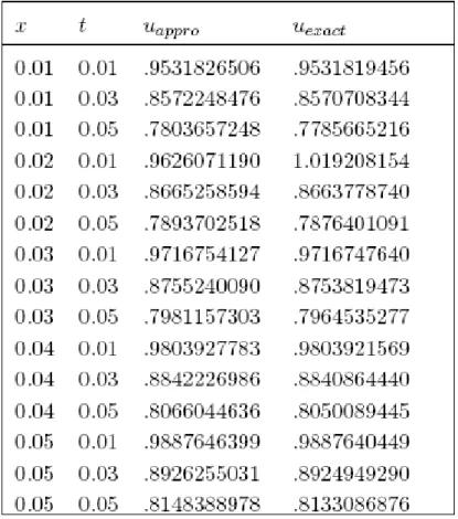
It is necessary to make tests for the approximate solution (series solution Eq.(18)) by making a comparison with the exact solution of linear heat equation. We take only four terms in each series, the approximate and exact solutions com-parisons can be found in Table 2, it seems that the series solution is confirmed with the exact solution.
Table 2. Comparison between the exact solution and the approximate solution (DTM) for Ex. 3.1.1
Example 3.1.2 In Eq.(2), taking = −2 and = 3, the following nonlinear heat equation is obtained,
(20) = − 23
We now solve Eq.(20) using DTM with the initial condition
(21) ( 0) = 1 + 2
2+ + 1
and the boundary conditions
(22) (0 ) = 1
6 + 1 (0 ) =
12 + 1 (6 + 1)2
Taking two-dimensional transform of Eq.(20), we have ( + 1) ( + 1) = ( + 1)( + 2) ( + 2 ) − 2 X =0 X− =0 X =0 − X =0 ( − − )( − − )( ) (23)
By equating the series form of Eq.(21) with Eq.(7), the initial transformation coefficients ( 0) ( = 0 1 ) can be obtained as follow.
(24) (0 0) = 1 (1 0) = 1 (2 0) = −2 (3 0) = 1 (4 0) = 1 By applying Eq.(25) into Eq.(23) , and so on, we can calculate another values of ( ) and by recursive method, some results are listed as follows in Table 3.
Table 3. Some values of ( ) Ex.3.1.2
Substituting all ( ) into Eq.(7), we have series solution as follows: ( ) = {1 + − 22+ 3+ 4− 25+ 6+ 7− 28+ 9+ }
+{−6 + 182 − 243 + 365 − 426 + 548 − 609 + } +{362− 362− 10822+ 28832− 18042− 32452 +75662− 43272− 64882+ 144392+ } + (25) The closed form of the first curly bracket is 1+2
2++1 the closed form of the
second curly bracket is (−6(1+2)2++1)2 the closed form of the third curly bracket is
36(1+2)
(2++1)33 and so on. Hence Eq.(25) can be written as
(26) ( ) = 1 + 2 2+ + 1 + −6(1 + 2) (2+ + 1)2 + 36(1 + 2) (2+ + 1)3 3+
The exact analytical solution of ( ) is given in [4]
(27) ( ) = 1 + 2
2+ + 6 + 1
In Table 4, we demonstrated how approximate solution of Eq.(20) with initial condition Eq.(21)is close to the exact solution by using DTM method. It is to be noted that only four terms were used in evaluating the approximate solution. We also achieved a very good approximation.
Table 4. Comparison between the exact solution and the approximate solution (DTM) for Ex.3.1.2
Example 3.1.3. In this example we consider the linear heat equation with = 0, = 2:
(28) − = 2 ∈ (0 1) 0
with boundary conditions and initial condition
(0 ) = (1 ) = 0 0 (29)
( 0) = sin() + (1 − ) 0 ≤ ≤ 1 (30) Taking the differential transform of Eq.(28), it can be obtained that
From the initial condition Eq.(30), (32) ( 0) = ⎧ ⎪ ⎪ ⎪ ⎪ ⎨ ⎪ ⎪ ⎪ ⎪ ⎩ ( + 1) = 1 −1 = 2 − ! = 3 7 11 ! = 5 9 13 0 otherwise.
Substituting Eq.(32) into Eq.(31), and by recursive method the results corre-sponding to ( ) ( = 0 1 2), we have ( 1) = ⎧ ⎪ ⎨ ⎪ ⎩ −+2 ! = 1 5 9 +2 ! = 3 7 11 0 otherwise. (33) ( 2) = ⎧ ⎪ ⎨ ⎪ ⎩ +4 2!! = 1 5 9 −2!!+4 = 3 7 11 0 otherwise. (34) ( 2) = ⎧ ⎪ ⎨ ⎪ ⎩ −3!!+6 = 1 5 9 +6 3!! = 3 7 11 0 otherwise. (35)
and so on. Substituting (32-35) into Eq.(7), the solution in a series form is ( ) = {( + 1) − 2+ (−1 6 3)3+ ( 1 120 5)5+ ( −1 5040 7)7 +( 1 362880 9)9+ ( −1 39916800 11)11 + } +{(−3) + ( 5 6 ) 3 + (− 7 120) 5 +( 9 5040) 7 + (− 11 362880) 9 + } +{( 5 2) 2+ (−7 12 ) 32+ (9 240) 52 (36) +(− 11 10080) 72+ ( 13 725760) 92 +( − 15 79833600) 112 + } +{(− 7 6 ) 3+ (9 36) 33+ (−11 720 ) 53 +( 13 30240) 73+ ( −15 2177280) 93 +( 17 299500800) 113 + } +
The closed form of the first curly bracket is sin() + (1 − ) the closed form of the second curly bracket is(−2 sin()) the closed form of the third curly
bracket is (242sin()) and so on. Hence Eq.(40) can be written as
(37) ( ) = sin() + (1 − ) + (−2 sin()) + (
4
2
2sin()) +
and, therefore, the exact solution
(38) ( ) = exp(−2) sin() + (1 − )
is readily obtained in [18]. It is obvious that the given boundary conditions justify the exact solution Eq.(38).
4.Conclusion
In this work, the differential transform method (DTM) was used for finding particular exact solution of a linear heat equation, and nonlinear heat equation that usually arises in mathematical biology with the initial conditions. It can be concluded that the DTM is very powerful and efficient technique for finding exact solutions for wide classes of problems. It is worth pointing out that the DTM presents a rapid convergence for the solutions.
All the examples in the text show that the results of the present method are in excellent agreement with those obtained by the Adomian’s decomposition method [6], Lie symmetry reduction method [9] and antireduction method [4]. The DTM has got many merits and much more advantage than these meth-ods. This method overcomes the difficulties arising in calculation of Adomian polynomials. The results also show that the DTM is a powerful mathematical tool for solving linear and nonlinear partial differential equations having wide applications in engineering and physics. The reliability of the methods and the reduction in the size of computational domain also make it applicable to many problems. As a result, this method can be applied to many complicated linear and nonlinear differential equations and does not require liberalization, discretization or perturbation.
References
1. J.D. Murray, Mathematical Biology, Springer, Berlin, 1993. 2. B.H. Gilding, R. Kersner, J. Diff. Eqns. 124 (1996) 27-79.
3. A.B. Cunningham, W.G. Charaklis, F. Abedeen, D. Crawford, Environ. Sci.Tech. 25 (1991) 1141-1148.
4. W. Fushchych, R. Zhdanov, Nonlinear Math. Phys.1 (1994) 60-64 5. S. Pamuk, Math. Models Meth. Appl. Sci. 13 (1) (2003) 19-33. 6. S. Pamuk, Appl. Math. Comput. 163 (2005) 89-96.
7. H.A. Levine, S. Pamuk, B.D. Sleeman, M. Nilsen-Hamilton, Bull. Math. Biol. 63 (5)(2001) 801-863.
8. B.D. Sleeman, A.R.A. Anderson, M.A.J. Chaplin, A mathematical analysis of a model for capillary network.
9. M. Euler, N. Euler, Sym. Nonlinear Math. Phys. 1 (1997) 70-78. 10. R.M. Cherniha, Sym. Nonlinear Math. Phys. 1 (1)(1997) 138-146. 11. Jang M.J., Chen C.L. , LiuY.C, Appl. Math. Comput; 2001; 121: 261-70. 12. Pukhov G.E. Differential transformations and mathematical modelling of physical processes. Kiev, 1986.
13. C.K.Chen, S. H. Ho, Appl. Math. Comput. 106 (1999) 171-179. 14. F.Ayaz, Appl. Math. Comput. 143 (2003) 361-374.
15. F.Ayaz, Appl. Math. Comput. 147 (2004) 547-567
16. Kurnaz A, Oturanç G, Kiri¸s M.E, Int J Comput Math;. 2005; 82: 369-80. 17. Abdel-Halim Hassan , I.H, Chaos, Solitons & Fractals; 2006;(in press)
18. M. Bayram, Fen ve Mühendislik için Nümerik Analiz, Aktif Yayınevi, Istanbul, 2002.