Repetition-rate stabilization of femtosecond stretched-spectrum fiber laser

(1)

REPETITION-RATE STABILIZATION OF

A FEMTOSECOND

STRETCHED-SPECTRUM FIBER LASER

A THESIS SUBMITTED TO THE DEPARTMENT OF PHYSICS

AND THE INSTITUTE OF ENGINEERING AND SCIENCE OF BILKENT UNIVERSITY

IN PARTIAL FULFILLMENT OF THE REQUIREMENTS FOR THE DEGREE OF

MASTER OF SCIENCE

By

Coşkun Ülgüdür August, 2008

(2)

ii

I certify that I have read this thesis and that in my opinion it is fully adequate, in scope and in quality, as a thesis for the degree of master of science.

. Asst. Prof. Dr. Fatih Ömer İlday

. Asst. Prof. Dr. Mehmet Özgür Oktel

. Instructor Hakan Altan

(3)

iii

Approved for the Institute of Engineering and Science:

. Prof. Dr. Mehmet B. Baray

(4)

iv

ABSTRACT

REPETITION-RATE STABILIZATION OF A FEMTOSECOND STRETCHED-SPECTRUM FIBER LASER

Coşkun Ülgüdür M.S. in Physics

Supervisor: Asst. Prof. Dr. Fatih Ömer İlday August, 2008

Passively modelocked lasers produce trains of femtosecond pulses, with the temporal separation between the pulses being determined by the length of the laser cavity. The repetition rate of the laser is inverse of this temporal separation. For a free-running laser, the repetition rate is very stable over short time scales (less than 1 ms), but drifts due to environmental effects on a longer time scale. For applications demanding a precise repetition rate to be maintained, such as optical frequency metrology, the laser needs to be locked to an RF or microwave reference source with a feedback loop acting on an actuator within the laser cavity.

In this work, repetition-rate stabilization of a “stretched-spectrum” fiber laser is reported, which corresponds to a new modelocking regime. As the name implies, the laser produces pulses undergoing periodic breathing of the spectra during a complete round trip through the cavity. To the best of our knowledge, this breathing is the strongest modification observed in a laser to date. It is noteworthy that even under such strong nonlinearity the laser is more robust than the regular stretched-pulse laser.

(5)

v

promising alternate to laser oscillators for frequency metrology applications and laser master oscillators in use with accelerator based next-generation light sources. After photodetection of the laser output, one of the upper harmonics of the laser is locked to a highly stable dielectric resonator oscillator (DRO) at 1.3 GHz. In order to reduce the environmental effects on the laser, a handmade encasing was developed and temperature control of the fibers in the cavity was implemented. Remarkably, the custom encasing of the laser dramatically improved the laser’s stability, outperforming the DRO up to a 5 kHz bandwidth. Since the heating-loop is not sensitive enough, latter upgrade does not decrease the phase noise of the laser, but ensures the temperature stability stays within limits in unclimatized environment. With the present setup, we observe a maximum locking range of a few kHz. The system has the potential to stay in-lock indefinitely, as long as the excessive perturbations on the system are prevented.

Keywords: Femtosecond fiber laser, stretched-spectrum fiber laser, laser phase noise, laser repetition rate, repetition-rate locking, phase-locked loop

(6)

vi

ÖZET

FEMTOSANİYE, GERİLMİŞ TAYFLI FİBER LAZERDE TEKRAR FREKANSININ DENGELENMESİ

Coşkun Ülgüdür Fizik Yüksek Lisans

Tez Yöneticisi: Asst. Prof. Dr. Fatih Ömer İlday Ağustos, 2008

Pasif olarak mod kilitli lazerler femtosaniye atım dizisi oluşturur. Bu atımların zamansal aralıklarını lazer kovuğunun uzunluğu belirler. Lazerin tekrar frekansı bu zamansal aralığın tersidir. Serbest hareketli lazerlerde, tekrar frekansı kısa zaman dilimlerinde (1ms’den daha az) oldukça kararlı olmasına rağmen çevresel faktörlerden dolayı daha büyük zaman dilimlerinde sapar. Optik frekans ölçme bilimi gibi tekrar frekansının kesin olarak belirli olması gereken uygulamalar için lazer bir geribesleme döngüsü ile RF ya da mikrodalga referans kaynağa kilitlenir.

Bu çalışmada yeni bir mod kilitleme rejimi olan gerilmiş tayflı bir fiber lazerin tekrar frekansının dengelenmesi bildiriliyor. İsmi işaret ettiği gibi, bu lazer kovuk içinde bir tur boyunca periyodik olarak daralıp genişleyen tayfa sahip atımlar üretir. Bilgimiz dahilinde bu daralıp genişleme şimdiye kadar bir lazer de gözlemlenmiş en güçlü değişimdir. Bu derece yüksek doğrusal olmayan etkilerde bile lazerin normal bir gerilmiş atımlı lazere nazaran daha sağlam olması dikkate değer.

Sağlamlığından cesaret alarak, gerilmiş tayflı fiber lazerin frekans ölçüm bilimi ve hızlandırıcı tabanlı yeni nesil ışık kaynağı uygulamalarında umut veren alternatif lazer

(7)

vii

1.3 GHz’de çalışan, yüksek derecede kararlı bir dielektrik çınlaç salıngacına (DRO) kilitlenir. Lazer üzerindeki çevresel faktörleri azaltmak için, el yapımı bir kutulama yapılmış ve kovuk içindeki fiberlerin sıcaklık kontrolü sağlanmıştır. Lazerin kutulanması kararlılığını dramatik olarak arttırmış, 5kHz bant aralığına kadar DRO’dan daha kararlı olmuştur. Sıcaklık kontrolü yeteri kadar hassas olmadığından, lazer faz gürültüsünü azaltmamış, fakat klimasız ortamda lazer sıcaklığının limitler içinde kalmasını sağlamıştır. Şu anki kurulumla, en fazla birkaç kHz kilitleme sınırı elde edilmektedir. Aşırı rahatsızlıklar engellenirse sistem potensiyel olarak sonsuza kadar kilitli kalabilir.

Anahtar sözcükler: Femtosaniye fiber lazer, gerilmiş tayflı fiber lazer, lazer faz gürültüsü, lazer tekrar frekansı, tekrar frekansı kilitleme, faz kilitli döngü

(8)

viii

Acknowledgement

Firstly I would like to thank my academic advisor Fatih Ömer İlday for his enthusiastic support of my thesis. His assistance at various points of the thesis carved the way it is finalized. Apart for his invaluable support, I would also like to thank him for the excellence of the working environment he provided in less than a year. The Ultrafast Lasers Group of Bilkent University would not be one of the pinnacles in its subject without his efforts to improve its facilities.

I am indebted to the members of the Ultrafast Lasers Group, Pranab Mukhopadhyay, Bastian Lorbeer, Alper Bayrı, İ. Levent Budunoğlu, Bülent Öktem, Kıvanç Özgören, Seydi Yavaş and Çağrı Şenel for providing a high standard scientific environment and for supporting me at various points of the thesis.

I want to express my special thanks to İ. Levent Budunoğlu for his friendship and support through the long days and nights of work. Thanks to our collaboration in laser noise measurements, most enlightening ideas come up during our discussions.

I am particularly grateful to Bülent Öktem for his support in numerical simulations part of the thesis. The initial parameters I used for my system were originally from his previous studies which helped me a great deal.

I wish to express my special thanks to Alper Bayri for his friendship and engineering support throughout the thesis. I am indebted to him for assisting me in the temperature control setup of the laser. His fast response in my orders of new equipment saved me days of invaluable time.

(9)

ix

discussions we had constantly for improving my setup.

I would like to thank Kıvanç Özgören for his friendship and for sharing his experience at various problems I encountered in the thesis.

Many thanks go to Dr. Aykutlu Dana for lending me his group’s power amplifier and for helping me about the problems I had with it.

I would also like to thank Paolo Sigalotti @FERMI Laser Group and Dr. Axel Winter @DESY for their introduction to phase-locked loops and noise phenomena in lasers. Their initial guidance helped me a lot throughout my studies.

I am grateful to Çağrı Şenel for his efforts on optimizing the numerical simulation algorithm for our needs and for writing the GUI of the simulation to let us use it efficiently.

Last but not the least I would like to thank all the members of Ultrafast Lasers Group for their lenience in my frequent use of public measurement devices and optic components toward the end of my thesis studies.

Finally, I wish to thank and acknowledge my thesis examination committee: Asst. Prof. Dr. Fatih Ömer İlday, Asst. Prof. Dr. Mehmet Özgür Oktel and Asst. Prof. Dr. Hakan Altan.

This work was supported by the Bilkent University, Department of Physics, Ultrafast Lasers Group and Turkish Scientific and Technical Research Council (TÜBİTAK).

(10)

List of Figures

2.1 (a) illustration of SHG. (b) Energy-level diagram SHG………..8

2.2 (a) illustration of SFG. (b) Energy-level diagram SFG………...9

2.3 (a) illustration of DFG. (b) Energy-level diagram DFG………10

2.4 (a) illustration of THG. (b) Energy-level diagram THG………12

2.5 Energy-level diagram of two-photon absorption………...15

2.6 Illustration and energy-level diagram of stimulated Raman scattering……….16

3.1 Illustration of (a) three-and (b) four-level lasing schemes……….30

3.2 Schematic of a fiber ring laser mode-locked via NPE………...40

4.1 Illustration of split-step Fourier method used for numerical simulations…….…….47

4.2 Screenshot of the simulator GUI………..…..48

4.3 Simulated spectrum of the pulse………52

4.4 Buildup of the pulse inside the simulated cavity over 50 roundtrips……….53

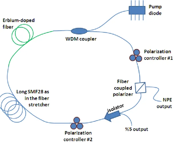
4.5 Schematic setup of the all-fiber stretched-pulse laser………54

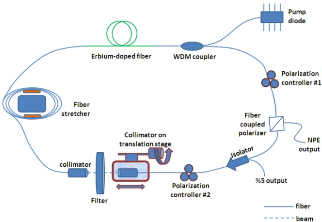
4.6 Schematic setup of the stretched-spectrum laser oscillator………...55

4.7 (a) Photo of the laser cavity including the fiber stretcher and free-space section, (b) Photo of the fiber laser inside the custom-made box. Temperature controller is set to keep the temperature inside the box at 26o_{C……….58}

4.8 Setup of an intensity autocorrelation……….60

4.9 Autocorrelation of the laser pulse train………..61

4.10 Measured optical spectrum of the pulse (simulation output – red)………62

4.11 Oscilloscope trace of the laser with 40 MHz repetition rate………..62

(13)

xiii

5.1 Time domain visualization of pulses from a mode-locked laser………...64

5.2 Time-to-frequency domain conversion of laser pulses………..65

5.3 Single comb line of the laser at 1.3 GHz………...65

5.4 Phase noise measurement setup……….67

5.5 Schematic of a phase noise measurement using SSA (from [40])……….…68

5.6 Single sideband phase noise for the laser oscillator in free-running mode…………70

6.1 Schematic setup of the PLL system………...72

6.2 Photograph of the system in operation. Error signal is monitored on the oscilloscope screen and the harmonic of the laser is monitored on the RF spectrum analyzer. Laser box is covered with thin metal sheet for temperature isolation………..73

6.3 Gain response of the power amplifier. Saturation after ±10 V DC input voltage with ±215 V DC supply………76

6.4 Performance record of the PLL (black line). Distorted lock (red line)………..79

6.5 Free-running laser and DRO phase noise comparison………...80

6.6 Phase noise comparison of the DRO and the laser at various conditions…………..82

6.7 Zoomed in section of the phase noise graph to show the PLL effect on the laser’s stability………..83

(14)

Chapter 1

1 Introduction

1.1. Brief History of Fiber Lasers

19th_{century hosts the origins of telecommunications. First the demonstration of telegraph}

by Samuel Morse in 1837, following the first telephone exchange operated by Alexander Graham Bell in 1878 initiated the rapid discoveries of communication means. James C. Maxwell’s clarification of “Maxwell’s Equations” in 1878 led to the discovery of radio waves by Heinrich Hertz in 1888 and in 1895 the first radio is demonstrated by Guglielmo Marconi. Early radio has a bandwidth 15 kHz and after more than a century the maximum bandwidth of wireless communication is still around a few hundred MHz. The reason is that free space propagation of signals is not suitable for reliable/fast communication links. The solution to this problem is to use a waveguide for light (information) propagation hence avoiding distortions present in free space. The basic phenomenon responsible for guiding of light in waveguides is total internal reflection. Optical fibers, the most common waveguides, were first fabricated uncladded in 1920s. However the real origin of fiber optics was not born until the first usage of cladding layer on optical fibers in 1950s. The use of cladding substantially improved the fiber performance. Nevertheless it is the use of low-loss silica in fiber fabrication that lets losses around 0.2 dB/km in the telecommunication wavelength, 1.5 µm.

(15)

The developments in optical fibers led not only to advancements in telecommunications, but also to the birth of a new field, nonlinear fiber optics. Studies of nonlinear phenomena in optical fibers such as Stimulated Raman- and Brillouin-scattering, optically induced birefringence, parametric four-wave mixing and self-phase modulation were conducted in 1970s [1-7]. An important milestone was that in 1973, it was suggested that optical fibers can support soliton-like pulses by the interplay between nonlinear and dispersive effects of fibers [8]. Optical solitons were first observed in a 1980 experiment [9] and led to further advances in the field of nonlinear optics. The field continued to grow in 1990s, especially after the fabrication of optical fibers doped with rare-earth elements (Erbium, ytterbium, etc). Fiber laser oscillators were the next phase in the field of nonlinear optics. However one problem was that soliton-like mode-locking regime in fiber lasers has severe limitations in terms of pulse energy and duration [10, 11]. Several other mode-locking regimes (dispersion-managed/stretched-pulse [12], similariton [13, 14], all-normal GVD [15]) have been demonstrated in recent years, which overcome many of these limitations. Using these new approaches, optimizing pulse energy, more than 10 nJ and optimizing pulse duration, pulses as short as 35 fs can be routinely obtained [16].

(16)

CHAPTER 1. INTRODUCTION 3

1.2. Motivation in Synchronization of Laser Oscillators

Passively modelocked lasers generate trains of femtosecond pulses, corresponding to a frequency comb in frequency domain. Although fiber lasers have superior short term stability (above 100 kHz), their long term performance suffers from various effects (i.e. rapid temperature change, pump power instabilities, upper state lifetime of the dopant in gain fiber, etc). This problem can be solved by locking the laser to an RF or microwave reference oscillator, hence improving its short term stability. As the laser pulses are depicted as frequency combs in frequency domain, synchronizing a laser to an ultrastable, but single frequency RF source would automatically turn out to be an ultrastable frequency source not at a single frequency but at discrete frequencies separated by the repetition rate of the laser. Clearly stabilizing a laser to an ultrastable source at particular frequency and getting the desired ultrastable frequency of choice would be much more efficient in every aspect rather than building a second RF source at the choice of frequency.

(17)

Chapter 2

2 Introduction to Nonlinear Optics

Much of ultrafast optics is based on understanding the basics of nonlinearities in optics. This chapter gives basic theories of nonlinear optics, followed by brief descriptions of major optical interactions due to nonlinearity. This chapter is mostly based on [17], further details can be found there.

2.1. Nonlinear Optical Susceptibility

Nonlinear optics emerged with the realization that optical properties of a material changes with light presence. Modification of optical properties in a material requires high intensities of light. At first this phenomenon seemed to be a problem for optical studies, but later became the foundation of laser technology.

The nonlinearity occurs in the sense that the response of a material to applied light is “nonlinear”. For example, high harmonic generation processes depends on power of the applied field strengths, i.e. square of the applied field leads to second harmonic generation, cube of the applied field leads to third harmonic generation.

(18)

CHAPTER 2. INTRODUCTION TO NONLINEAR OPTICS 5 Polarization has a key role in describing nonlinear optics. It shall be examined in section 3.1 that the nonlinear wave equation is,

1

2.1

where c is the speed of light in vacuum and n is the linear refractive index. One can see from the above equation that whenever term is nonzero, the charged particles are accelerated and as Larmor’s theorem stated, charged particles under acceleration are the source of electromagnetic radiation.

In conventional optics, polarization of a material depends on the field strength as;

2.2

where is the linear susceptibility of the material. However, nonlinear response of materials does not satisfy Equation (2.2). The applied field causes anharmonic motion of bound electrons in a material as a result polarization satisfies the more general relation;

… 2.3

(19)

where and are known as the second and third-order nonlinear optical

susceptibilities. In these generalized equations (Equations. (2.3) and (2.4)), or , the linear term is the dominant contribution to the overall polarization of the material. Other terms are the correction factors required for compensation of very high applied field effects on polarization. As one might expect, the propagation of light in fiber is ruled by Maxwell’s equations from which wave equation is emerged. Nonlinear terms in polarization also transform the wave equation into a nonlinear differential equation which has special solutions (light propagation in fibers will be examined in greater detail in later sections). , the second order nonlinear polarization is responsible for effects like

Second-Harmonic Generation whereas , the third order nonlinear polarization

triggers effects like Kerr Nonlinearity, both of which will be explained in detail in subsequent sections. occurs in media with molecular level inversion symmetry (centrosymmetric media), henceit is zero for liquids, gases, amorphous solids(i.e. glass) and most crystals because they have no inversion symmetry. However can occur both in centrosymmetric and noncentrosymmetric media. This distinction is the reason that in spite of high intensities, there is no second harmonic generation in a laser cavity consisting of only fibers and free-space; and one needs birefringent crystals inside a laser cavity to create second harmonic of the pulse. Similarly it is the reason that weaker polarization term ( ) has the dominant nonlinear effect in a fiber laser. i.e. Kerr effect.

A simple order of magnitude estimate of susceptibility values might be calculated as follows; the second order polarization term would be significant enough with respect to linear term when the amplitude of the applied field strength E is on the

(20)

CHAPTER 2. INTRODUCTION TO NONLINEAR OPTICS 7 order of atomic electric field strength Eat=e/ao2 where e is the electron charge and ao=ћ/me2 is the Bohr radius of the hydrogen atom (ћ is Planck’s constant divided by 2π and m is the electron mass). Substituting the values of physical constants ћ, m and e from literature,Eat is found to be 6. 66 10 m/V. Thus the second-order susceptibility χ(2) _{would be on the} order of χ(1)/ Eat. χ(1) is almost unity for condensed matter, so χ(2) value for condensed matter is given as;

χ(2) ≈ 2.09 x 10-11 m/V (2.5)

Similarly, χ(3)would be on the order of χ(1)/ Eat2, which has a value for condensed matter;

χ(3) ≈ 4.2 x 10-23 m2/V2 (2.6)

These order of magnitude values of linear susceptibility terms would be a hint why nonlinearity requires high intensities to govern light propagation inside optical media.

2.2. Nonlinear Optical Interactions

In this section a number of nonlinear optical interactions will be introduced briefly and be explained how they can be integrated into Equation (2.3), the general polarization equation. However some of these interactions are beyond the scope of this thesis, hence only the interactions that govern the physics in fiber lasers will be examined in detail in later sections.

(21)

Second-Harmonic Generation (SHG):

(a) (b)

Figure 2.1. (a) Illustration of SHG. (b) Energy-level diagram SHG.

In second-harmonic generation two photons at same frequency ω are vanished and a photon at frequency of 2ω is created in a single quantum mechanical process. This is illustrated in Figure 2.1.a. In Figure 2.1.b, the solid line is the ground state and the dashed lines are the virtual levels, which represent essentially the combined energy of one of the energy eigenstates of the atom and of one or more photons of the radiation field.

In theory a laser beam with electric field;

. . 2.7

is incident upon a crystal with a nonzero second order susceptibility χ(2) then the nonlinear polarization that is created in such a crystal is given as;

2 . . 2.8 ω 2ω ω ω ω 2ω χ(2)

(22)

CHAPTER 2. INTRODUCTION TO NONLINEAR OPTICS 9 In Equation 2.8, the second-order polarization consists of a contribution at zero frequency and a contribution at frequency 2ω. According to Equation (2.1), the nonlinear wave equation, contribution at frequency 2ω leads to the generation of radiation at the second-harmonic frequency. However contribution at zero frequency cannot lead to the generation of any electromagnetic radiation because its second time derivative is zero.

Sum-Frequency Generation (SFG):

(a) (b)

Figure 2.2. (a) Illustration of SFG. (b) Energy-level diagram SFG

Sum-frequency generation is analogous to that of second-harmonic generation, except that in SFG the two input frequencies are different as in Figure 2.2.a. If a laser beam with electric field E(t) (Equation (2.7)) is incident upon a crystal with nonzero χ(2), the nonlinear polarization that is created in SFG process is given by;

2 2.9 ω3= ω1+ ω2 ω2 ω1 χ(2) ω2 ω1 ω3

(23)

Difference-Frequency Generation (DFG):

(a) (b)

Figure 2.3. (a) Illustration of DFG. (b) Energy-level diagram DFG

In difference-frequency generation, difference frequency of applied fields is generated (Figure 2.3). The process is described by the nonlinear polarization;

2 2.10

To consider the general picture of second order frequency generation, assume an optical field with electric field;

. . 2.11

is incident upon a nonlinear medium with nonzero χ(2). Then the nonlinear polarization created in such a medium is of the form;

ω3= ω1- ω2 ω2 ω1 χ(2) ω1 ω3 ω2

(24)

CHAPTER 2. INTRODUCTION TO NONLINEAR OPTICS 11

2 2

_. ₂ _2.12

Each of the complex amplitude term of various frequency components of this nonlinear polarization corresponds to different nonlinear process. First two terms would be the SHG form, third one is the SFG form and the last one is the DFG form. However, one should note that no more than one of these frequency components will be present with any appreciable intensity in the radiation generated by the nonlinear optical medium. The reason is that nonlinear polarization processes can produce decent output signal only if a certain phase-matching condition is satisfied.

Third-Order Polarization:

Third-order contribution to the nonlinear polarization in a nonlinear media with nonzero χ(3) is;

2.13

For the general picture, an applied electric field consisting three frequency components is assumed to be incident upon the nonlinear media;

(25)

However in this case calculated E3(t) contains 44 different frequency components

corresponding to distinct mixing processes, hence the expression for P3(t) will be very

complicated. For the purpose of simplicity and sufficiency, the simple case in which the applied field is in single frequency is considered;

2.15

Through the use of the trigonometric identity, 3 , the

nonlinear polarization can be found as;

3 2.16

In Equation (2.16) each term corresponds to a different nonlinear process which will be briefly introduced below.

Third-Harmonic Generation (THG):

(a) (b)

Figure 2.4. (a) Illustration of THG. (b) Energy-level diagram THG

ω 3ω ω χ(3) ω ω 3ω ω

(26)

CHAPTER 2. INTRODUCTION TO NONLINEAR OPTICS 13 The first term in Equation (2.16) describes a nonlinear response at frequency 3 created by an applied field at frequency . This term defines the process of third-harmonic generation, which is described in Figure 2.4. In this process three photons at frequency are destroyed and one photon at frequency 3 is created in a single quantum mechanical process.

Intensity-Dependent Refractive Index:

The second term in Equation 2.16 describes a nonlinear contribution to the polarization at the frequency of the incident field . Hence it leads to a nonlinear contribution to the refractive index experienced by the incident field at frequency . The nonlinear refractive index can be represented as;

2.17

where is the linear refractive index and 3

8 2.18 is an optical constant that decides the strength of the optical nonlinearity and where

| | 2.19

(27)

This process is also known as Kerr nonlinearity which plays an important role in fiber lasers.

All of the processes described up to this point are examples of parametric processes. In parametric processes the initial and final quantum mechanical states of the system are same. Conversely, processes in which the initial and final quantum mechanical states are distinct real levels are known as nonparametric processes. Mainly two differences are there between parametric and nonparametric processes. The former one is always described by a real susceptibility, whereas the latter can be described by a complex susceptibility. The second difference is that photon energy is conserved in a parametric process; conversely photon energy need not be conserved in a nonparametric process. The following two nonlinear processes are examples of nonparametric processes.

Saturable Absorption:

Many materials’ absorption coefficient decreases when measured using high intensity lasers. The dependence of the measured absorption coefficient on the intensity I of the incident field is given by;

1 ⁄ 2.20

where is the low-intensity absorption coefficient and is the saturation intensity.

Saturable absorption is one of the key concepts in mode-locking of lasers hence its role in laser operation will be described in detail in Section 3.3.

(28)

CHAPTER 2. INTRODUCTION TO NONLINEAR OPTICS 15

Two-Photon Absorption:

Figure 2.5. Energy-level diagram of two-photon absorption.

In two-photon absorption (illustrated in Figure 2.5) an atom has a transition from its ground state to an exited state by the simultaneous absorption of two photons. In contrast with linear optics, the absorption coefficient that describes two-photon absorption increases linearly with laser intensity as;

2.21

where σ is a coefficient that describes two-photon absorption. In addition, the atomic transition rate due to two-photon absorption is proportional to the square of the field intensity, since ⁄ ω, or to; ħ

ħ 2.22

ω ω

(29)

Stimulated Raman Scattering:

(a) (b)

Figure 2.6. Illustration and energy-level diagram of stimulated Raman scattering.

In stimulated Raman scattering (illustrated in Figure 2.6) a photon at frequency vanishes and a photon at the Stokes frequency forms. In this picture is the frequency that the atom is left in an excited state with energy ħ after the scattering. The stimulated Raman scattering process is very efficient compared to normal or spontaneous Raman scattering where both an exited atom’s vibration and a photon is annihilated to have a photon at the anti-Stokes shifted frequency

ωs= ω- ωv ω Raman medium ω1 ωv ωs= ω- ωv

(30)

Chapter 3

3 Theory of Fiber Lasers

To understand and describe the propagation of laser light in a dispersive optical medium, it is necessary to take the theory of electromagnetic wave propagation into account. This chapter gives derivation of basic wave equation, followed by the theory of pulse propagation in dispersive optical medium. Discussion of amplification in fibers and mode-locking will conclude the section. This chapter is mostly based on [18,19], further details can be found there.

3.1. Ultra-short Pulse Propagation in Fibers

Like all electromagnetic phenomena, the propagation of pulses in optical fibers is ruled by Maxwell’s equations;

. 3.1 . 0 3.2 3.3

(31)

where B and D are magnetic and electric flux densities, respectively, and H and E are the corresponding magnetic and electric field vectors. Since there are no free charges in optical fibers, free charges and current density vanish. The flux densities are related to electric and magnetic field through the relations given by;

3.5 3.6

Where is the vacuum permittivity, is the vacuum permeability, and P and M are induced electric and magnetic polarizations respectively. For an optical medium M is zero. Using the mathematical identity . and taking the curl of both sides of Equation (3.3) gives;

. 3.7

Using Equations (3.4), (3.5) and (3.6) one can obtain;

3.8

Substituting Equation (3.8) in (3.7) gives an equation depending on E and P only;

(32)

CHAPTER 3. THEORY OF FIBER LASERS 19 Since there are no free charge carriers, . 0 and using the relation 1⁄ , Equation (3.9) can be reduced to the wave equation;

1

3.10

A few assumptions need to be made before solving Equation (3.10). First the nonlinearity in P is treated as a small perturbation. Second, the optical field maintains its polarization along the fiber length so that a scalar approach is valid. Third, the polarization response of the field is instantaneous. This is valid for a nonlinear response that is electronic in nature, since the reconfiguration time of the electron cloud is significantly smaller than the period of the optical light wave. The contributions of molecular vibrations to the nonlinear part of the polarization (the Raman effect) is neglected for now and will be discussed later in this section.

The third assumption lets the expansion of the induced polarization in a series of powers of instantaneous electric field;

, , , , … 3.11

The electric field has a time structure that has a rapidly and slowly varying component. The slow timescale is the width of the pulse, which is typically on the order of 100 fs. The fast timescale is the optical cycle, which is on the order of ⁄ 5 fs. Hence it is useful to separate the timescales of electric field and polarization components in the form;

(33)

, 1 2 , exp . . 3.12 1 2 , , exp . . 3.13 , 1 2 , exp . . 3.14 , 1 2 , exp . . 3.15 Only the real part of the above equations is physically relevant, hence complex conjugate parts will not be stated anymore. Here, is the unit vector perpendicular to the propagation direction, which can be ignored because of the assumption that the polarization is maintained during the propagation through the fiber. , and _/ , are the slowly varying envelopes of the corresponding components. For future simplifications, the dependencies on and (modal pattern) from that on and (propagation) are separated. This is appropriate because the transverse mode structure in the fiber is to first order independent of propagation length and time. The quickly varying parts in both and are expressed as a plane wave which propagates in the -direction and is of definite frequency

and associated wave number ⁄ .

The assumption in Equation (3.11) lead to the approximation of nonlinear polarization [18]

, , , 3.16

(34)

CHAPTER 3. THEORY OF FIBER LASERS 21

, 3

4 | , | 3.17 To obtain the wave equation for the slowly varying amplitude , it is useful to work in the Fourier domain. However, because is intensity dependent, it is not possible to apply a Fourier transform. In the subsequent approach perturbative assumption of is used, hence can be treated as locally constant. Substituting Equations (3.12) through (3.15) in Equation (3.10), the Fourier transform Ẽ , , defined as;

Ẽ , , exp 3.18

is found to satisfy the Helmholtz equation;

, Ẽ , 0 3.19

with the dielectric function given by

1 3.20

Equation (3.19) can be solved by using the method of separation of variables. A solution of the form;

(35)

which is the Fourier transform of Equation (3.13), is assumed; where , is a slowly varying function of and , is the modal distribution of the pulse in the fiber. Further calculations (see [18] for details) leads to two equations for , and , ;

0 3.22

2 0 3.23

, is assumed to be a slowly varying function of , its second derivative was neglected. The wave number is determined by solving the eigenvalue equation for the fiber modes (see [18] for details). The dielectric function in Equation (3.22) is approximated by;

∆ 2 ∆ 3.24

where ∆ is a small perturbation given by the nonlinearity of the refractive index and the absorption and gain in the fiber;

∆ | |

2 3.25

The solution for the modal distribution , is not affected compared to the case without the perturbation. However, the eigenvalue solution becomes;

(36)

CHAPTER 3. THEORY OF FIBER LASERS 23 ∆ 3.26

∆ ∆ | , |

| , | 3.27

Only single-mode fibers are considered here, , corresponds to the modal distribution of the fundamental fiber mode HE11 given by [18]

, , 3.28 inside the core and;

, / exp , 3.29

outside the core. This modal distribution is cumbersome in practice, is approximated by the Gaussian distribution;

, exp / 3.30

where the width parameter is obtained by curve fitting.

Rewriting Equation (3.23) by using (3.26) and approximating by

2 gives;

(37)

After this point, one can go back to the time domain by taking the inverse Fourier transform of Equation (3.31), and obtain the slowly varying envelope function , . Since an exact functional form for is not known, it is useful to expand it in a Taylor series around the carrier frequency as;

1 2 1 6 3.32 where and, 1,2, … 3.33

The cubic and higher-order terms in the expansion are negligible it the pulse duration in the ps-range. For femtosecond pulses however, third-order dispersion has to be taken into account. Using a similar expansion for ∆ , substituting both expansions in Equation (3.31) and taking the inverse Fourier transform it by using;

, 1

2 , exp d 3.34

gives the resulting equation for , ;

(38)

CHAPTER 3. THEORY OF FIBER LASERS 25 The effect of fiber loss and nonlinearity is included in the term ∆ and can be evaluated using Equation (3.27). Using / and assuming , in (3.27) does not change much over the pulse bandwidth lead to;

2 2 | | 3.36 with the nonlinear parameter defined as;

3.37

where is the effective mode area of an optical fiber. Evaluation of it requires the use of the modal distribution , . If , is approximated by a Gaussian distribution,

. Typically, ranges between 1-100 μm2 in the 1.5 μm region.

A transformation of Equation (3.36) into a reference frame moving at the group velocity 1⁄ of the pulse envelope leads to;

2 2 | | 3.38

where . Because of resemblance this equation is called the nonlinear Schrödinger equation (NLSE) and is used to describe the propagation of ps-range pulses through optical fibers, taking into account chromatic dispersion by , fiber losses by and fiber nonlinearities by γ.

(39)

It is useful to introduce two length scales, dispersion length LD and nonlinear length LNL. This makes it possible to compare the relative strengths of effects over the propagation distance. These lengths are defined as;

, 1 3.39

Here is the initial pulse length and is the pulse peak power. Rewriting equation 2.29 with these new parameters leads to;

2 2 | | 3.40

where the absolute square of the field now gives power instead of intensity, through the

transformation , , ⁄ .

Unfortunately, some of the assumptions used in deriving the NLSE are not valid for ultra-short pulses (100 fs regime). The bandwidth needed to support such ultra-short pulses is so large that third-order dispersion effects can no longer be neglected. Furthermore the assumption that the fiber nonlinearity responds instantaneously compared to the pulse duration is no longer supported. In addition, the contribution to from the Raman effect becomes significant, as it occurs over a time scale of around 60 fs. The next few pages in this section will deal with the extension of the NLSE to include these effects.

For pulses with a wide spectrum, the Raman effect can amplify low-frequency components of a pulse by energy transfer from the high-frequency components of the same pulse. As a

(40)

CHAPTER 3. THEORY OF FIBER LASERS 27 result of it, a red-shift of the optical spectrum of the pulse, a feature referred to as

Raman-induced frequency shift takes place. To include this effect, one needs to re-evaluate the

nonlinear polarization equation (3.10). Any related effects are still neglected as they require phase-matching. The scalar form of nonlinear polarization is given by;

, 3

4 , | , | 3.41

which includes the nonlinear effects in a response function where is defined similarly to a time-delayed delta function such that 1.This corresponds to ∆ . The upper limit of integration extends up to to ensure causality. Somewhat lengthy algebra leads to the expression (see [18] for details);

2 6

1 2

, | , | 3.42

For pulse durations that can contain many optical cycles (pulse width 100 fs), it is possible to simplify Equation (3.42) by setting 0 and / and using a Taylor expansion of the form;

(41)

The following equation is acquired;

2 2 6 | | | |

| |

3.44

where a reference frame moving with the group velocity is used similar to the case in Equation (3.38). is defined as the first moment of the nonlinear response function . This latest form of the NLSE also contains the third-order dispersion ( term), the effect of self-steepening ( term) caused by the intensity dependence of the group velocity and the Raman-induced frequency shift ( term) caused by the delayed Raman response. A numerical value has been deduced experimentally as 3 fs for the spectral region around 1550 nm.

Solution of the NLSE is pretty straight-forward for negative . For this case, the solution does not change along the fiber length. Such a phenomenon is called a solitary wave solution. It was first observed in 1834 by Scott Russell in water waves propagating with undistorted phase over several kilometers through a canal.

The physical origin for optical solitons is a balance of dispersion and nonlinearity. Equation (3.38) can be rewritten as;

| |

(42)

CHAPTER 3. THEORY OF FIBER LASERS 29 with the assumption of no fiber losses ( 0). If both and are negative, there can be a combination of pulse duration (the parameter responsible for the magnitude of ) and pulse energy (the parameter responsible for magnitude of ), such that both terms cancel and 0. This means that, the envelope of the pulse does not change while propagating through a fiber if fiber losses and higher order nonlinear effects are neglected. The solution is characterized by a hyperbolic secant pulse shape;

| | | |sech 3.46

3.2. Amplification in Rare-Earth Doped Fibers

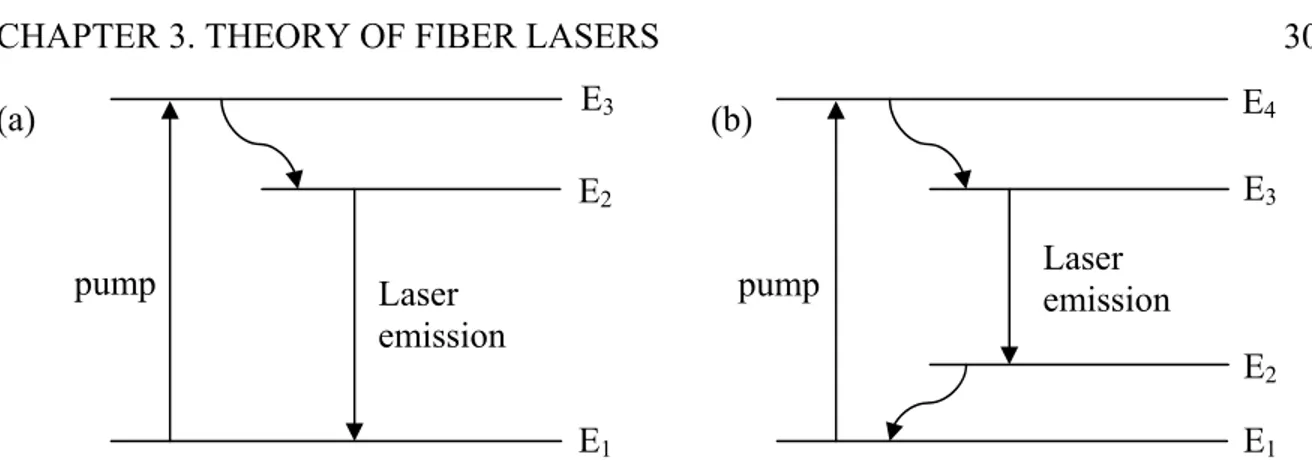
Optical fibers can amplify light at correct wavelength through stimulated emission. This is done by optically pumping the amplifier fiber to obtain population inversion. Depending on the energy levels of the dopants (rare-earth elements like erbium, ytterbium, neodymium, samarium and thulium), lasing schemes can be classified as a three- or four-level scheme (Figure 3.1). In either case, dopants absorb pump photons to reach an excitation stage than relax rapidly into a lower-energy excited state. The life time of this intermediate state is usually long (around 10ms for erbium and 1ms for ytterbium), and the stored energy is used to amplify incident light through stimulated emission. The difference between the three- and four-level lasing schemes is the energy state to which the dopant relaxes after each stimulated-emission event. In the case of a three-level lasing scheme, the dopant ends up in the ground state, whereas it occupies an exited state in the case of a four-level lasing scheme. Erbium-doped fiber lasers and amplifiers make use of three-level scheme.

(43)

(a) (b)

Figure 3.1. Illustration of (a) three-and (b) four-level lasing schemes

Optical pumping creates the necessary population inversion between two energy states and provides the optical gain. Using the appropriate rate equations (see [20] for details), the gain coefficient for a homogeneously broadened gain medium can be written as;

1 / 3.47 where is the peak gain value, is the frequency of the incident signal, is the atomic transition frequency and is the optical power of the signal being amplified. The saturation power is mainly influenced by the parameters such as the fluorescence time T1 (in the range of 1 μs to 10 ms for commonly used dopants) and the transition cross section σ. The parameter is the dipole relaxation time and is usually on the order of 0.1 ps for fiber amplifiers.

If the saturation effect is neglected in Equation (3.47), the gain reduction for frequencies off the transition frequency is governed by a Lorentzian profile. The gain bandwidth ∆v is

E3 E2 E1 Laser emission pump pump E4 E3 E2 E1 Laser emission

(44)

CHAPTER 3. THEORY OF FIBER LASERS 31 defined as the full width at half maximum (FWHM) of the gain spectrum , given for a Lorentzian spectrum as;

∆ ∆

2

1

3.48

However, the actual gain spectrum of a fiber laser can deviate significantly from the Lorentzian profile. The shape and the width of the gain spectrum are sensitive to core composition (i.e. the amorphous nature of the silica and the presence of other co-dopants such as aluminum or germanium).

In the latter part of this section, the effects of gain provided by dopants for the NLSE will be examined.

The lasing process can be approximated by a two-level system, as the lifetime of the first upper state is significantly shorter than the lifetime of the state from which stimulated emission takes place. The dynamic response of a two-level system is governed by the Maxwell-Bloch equations [20]. The starting point is the wave equation (3.10), but the induced polarization has to include a third term representing the contribution of dopants. Using the slowly varying envelope approximation similar to Equation (3.14);

, 1

2 , exp . . 3.49 The slowly varying part is dictated by the Bloch [20] equations which relate the population inversion density to the polarization and electric field;

(45)

, ,

,

ħ , 3.50 1

ħIm , . , 3.51

where is the magnetic dipole moment, is the atomic transition frequency, and , is the slowly varying amplitude defined as in Equation (3.14).

Following the same method in previous section for the derivation of NLSE, the NLSE (3.36) is modified as;

2 2 | | 2 , 3.52

where the angled brackets denote an averaging over the mode profile | , | . The preceding three equations (3.50)-(3.52) need to be solved for pulses of a duration comparable to the relaxation time (0.1 ps). The analysis is simplified considerably for longer pulses, where the dopants respond so fast that the induced polarization follows the optical field adiabatically (see [20] for details). Dispersive effects can be included by working in the Fourier domain and defining the dopant susceptibility as;

, , , 3.53

(46)

CHAPTER 3. THEORY OF FIBER LASERS 33 , / 3.54

Similar approach used in deriving in NLSE can be performed, provided the dielectric constant is modified to take into account. This leads to a change in Equation (3.25);

∆ | |

2 3.55 The major difference is that ∆ in Equation (3.27) becomes frequency dependent due to . Hence, when transforming the optical field back to the time domain, both and ∆ must be expanded into a Taylor series. The resulting equation is found after somewhat lengthy algebra (see [21] for details);

2 2 | | 2 1 1 3.56 where 2 1 2 1 3.57 2 3 1 3 1 3.58 and the detuning parameter . The gain is given by;

(47)

, , | , |

| , | 3.59

Spatial averaging is due to the use of Equation (3.55) in (3.27). Equation (3.56) shows that gain not only affects the group velocity of the pulse ( ), but also the chromatic dispersion through the effective . The change in the group velocity is usually negligible, since the second term is smaller on the order of 10-4 compared to . In contrast, not so for since near the zero-dispersion wavelength of the optical fiber, the two terms can become comparable. Even in the special case of 0, does not reduce to , in fact it comes down to;

3.60

which is a complex parameter caused by the gain induced by the dopants. The physical origin of this contribution is called gain dispersion which is due to the finite gain bandwidth of doped fibers. Equation (3.60) is a result of the parabolic-gain approximation used in the derivations in [21].

The integration of Equation (3.59) is difficult since the inversion profile depends on the spatial coordinates , and and the mode profile | , | because of gain saturation. However, in practice only a small portion of the fiber core is actually doped. If both the mode and dopant intensity are nearly uniform over the doped region, can be assumed to be constant there and zero outside. Then Equation (3.59) can easily be integrated leading to;

(48)

CHAPTER 3. THEORY OF FIBER LASERS 35 , , 3.61

where is the fraction of mode power within the doped region. Using Equation (3.61) and (3.51), the equation for gain dynamics can be found;

| |

3.62

where is the small signal gain. For most fiber amplifiers the fluorescence time is long compared to the pulse width and hence spontaneous emission and pump power changes do not occur over the pulse duration, Equation (3.62) can be integrated, leading to;

, exp 1 | , | 3.63

where is the saturation energy which is on the order of 1μJ for fiber amplifiers. This energy level is not reached in the lasers and fiber amplifiers, so gain saturation is negligible over the pulse duration. However, for a long pulse train, saturation can occur over timescales longer than . The saturation is determined by the average power in the

amplifier system 1 / .

Pulse propagation in an optical fiber is governed by a generalized NLSE (3.36) with coefficients and that are not only complex but also vary along the fiber length. In the specific case where the detuning parameter is zero, the NLSE can be written as;

(49)

2 | | 2 3.64

where is the reduced time. The term accounts the decrease in gain for spectral components of the pulse far from the gain peak. This equation is called the “Master Equation of Mode-locking” [22].

3.3. Modelocking of Fiber Lasers

Mode-locking a laser leads to ultra-short pulses with duration of a few-ps or less. For this purpose a phase relation between the many longitudinal modes which can exist in a laser cavity should be found. In this section, the principle of only passive mode-locking will be introduced using an artificial saturable absorber, as this is the method implemented in the erbium-doped fiber laser used in this thesis.

An electromagnetic pulse propagating in a laser cavity can be denoted by a superposition of plane waves with different wavelengths. The possible wavelengths of the longitudinal modes are given by the condition;

2 3.65

where is the wavelength of the longitudinal mode and is the cavity length. A large number of modes of different frequency can exist at the same time and each will be independent in phase and amplitude. Thus the total electric field in the cavity is given by the sum of the field of all modes;

(50)

CHAPTER 3. THEORY OF FIBER LASERS 37

, , _, , _, _, 3.66

where , is the complex amplitude of the n-th mode and its phase. Assuming equal

amplitude for all modes, the intensity is;

, , , | | Ω 3.67

where

Ω 3.68

being the frequency difference between two consecutive modes. If all modes have fixed phase relation, Equation (3.67) simplifies to;

, , , | | Ω 3.69

The second exponential part in the above equation will be 1 for all terms of the sum if the condition;

Ω 2 2 , 0,1,2, … 3.70

(51)

| | 3.71

The temporal and spatial distances of neighboring pulses as a function of the intensity can be derived from Equation (3.70) as;

∆ 2 , ∆ 2 3.72

This means the intensity maxima repeat with the revolution time of the laser resonator and there is one maximum inside the cavity at any time. Due to a fixed phase relation between the modes in the cavity, pulses with peak intensity will grow, proportional to the square of the number of modes. To calculate the FWHM of the pulses, the superposition of N modes is assumed to be similar to the interference of N planar waves at a fixed time 0. Using geometric series;

sin ₂Ω

sin Ω₂ 3.73

The FWHM of the pulses can be derived from the above equation as;

∆ 1

2 ∆

1 2 1

3.74

The pulse width decreases with the number of superposed modes and is directly proportional to the revolution time of the laser cavity.

(52)

CHAPTER 3. THEORY OF FIBER LASERS 39 A phase relation between superposed modes can be achieved by a modulation of the gain of the cavity with the difference frequency Ω of subsequent modes. All techniques to get a mode-lock rely on this principle. Due to loss modulation, the electromagnetic field in the cavity gets additional time dependence;

, _, cosΩ 3.75 , 1 2 Ω Ω , 1 2

The above equation hints that the time dependence induces sidebands in every mode whose frequencies coincide with the one of the neighboring modes. Since this is valid for the total bandwidth, a phase synchronization so called “mode-lock” between all longitudinal modes is achieved.

There are several ways to have mode-lock state in a laser. They are categorized by the method of how gain modulation is done. If an actively driven device, i.e. a switch or amplitude modulator is used, it will be active mode-locking, if a passive device like a saturable absorber is used, it will be passive mode-locking. However for the relevance of this thesis, only a special case of passive mode-locking will be explained in greater detail in the subsequent part.

(53)

In passive mode-locking the nonlinear component used to make mode-locked lasing more favorable than continuous-wave (cw) lasing simply introduces a higher loss at low power so that a short pulse with higher peak power experiences a stronger net gain.

Fiber lasers can also be mode-locked by using intensity dependent changes in the state of polarization when the orthogonally polarized components of a single pulse propagate inside an optical fiber. The polarization of the intense center of the pulse is rotated more than the less intense wings.

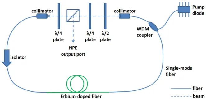
Figure 3.2. Schematic of a fiber ring laser mode-locked via NPE

The mode-locking process can be understood considering a fiber laser built in a ring configuration as shown in Figure 3.2. The pulse is linearly polarized after the polarizing beam splitter (PBS). The quarter wave plate following the PBS set the polarization to be

(54)

CHAPTER 3. THEORY OF FIBER LASERS 41 slightly elliptical, such that Kerr effect in the fiber section has a notable effect on the polarization of the pulse. After the fiber section, the polarization of the pulse center will differ from the polarization of the wings. The combination of quarter- and half-wave plate makes the polarization to be linear in the central part of the pulse, so the center of the pulse passes through the PBS cube and the wings are reflected out of the cavity through the nonlinear polarization evolution (NPE) port. The overall effect of the waveplates, PBS cube and fiber is shortening of the pulse after each round trip, with the PBS effectively acting as a saturable absorber.

The pulse at the beginning of the fiber section after free-space has to have elliptical polarization. The reason is explained as: The main contributors to the intensity dependence of the polarization evolution are self-phase and cross-phase modulation (SPM and XPM). Assuming the two eigenmodes are polarized along the - and -axis with intensity levels and , the total phase delays Φ and Φ along the axis can be obtained by adding the linear phase delays 2 and 2 as well as self- and cross-phase modulation term [23];

Φ 2

3 2 3.76

Φ 2

3 2 3.77

where is the fiber length. The difference of the above equations gives the net phase shift between the two axes;

(55)

∆Φ Φ Φ 2

3 2 3.78 Equation (3.78) suggests that circular input polarization does not lead to any intensity dependent phase shift, so the polarization of the pulse has to be elliptical when entering the fiber section of the cavity. This is achieved by the quarter-wave plate after the PBS cube.

(56)

Chapter 4

4 Laser Oscillator System and Characterization

Ultrafast fiber lasers have the potential to serve as master oscillators in accelerators. Pulse durations on the order of 100 fs are required to work in this area, hence the most promising candidate is a passively mode-locked laser through nonlinear polarization evolution. Noting these arguments, an erbium-doped fiber laser is selected to be used as the oscillator in this thesis for which components are widely available due to its operation at the telecommunication wavelength of 1550 nm.

4.1. Stretched-pulse vs. Stretched-spectrum Type Similaritons

One stability limit for mode-locking is the amount of nonlinear phase shift the pulse accumulates during one round trip. A soliton, the stable solution to the NLSE as discussed in Section 3.1, becomes unstable if it accumulates a phase shift of 2π or more per round trip. This would mean a soliton-laser’s output power is limited to very small levels.

In an approach first found by Tamura et.al. in 1993 [24], alternating pieces of normal and anomalous dispersion fibers were combined to have breathing of the pulse duration one round trip, making the pulse short in the middle of the normal and anomalous pieces of the fiber cavity. This results in an effective decrease in peak power, as the pulse is only short

(57)

for a small portion of the fiber cavity. Since nonlinear effects are peak power dependent, the nonlinear phase shift accumulated per round trip is considerably decreased to the case of a soliton. In other words pulse energy that the laser can sustain before becoming unstable is increased, thus laser has a higher output power. A further increase in the output power can be achieved by construction a laser such that the net dispersion of the cavity is not zero but slightly positive. Therefore the pulse will not reach the transform limit inside the cavity and will always have a positive chirp. This will further increase the maximum energy of the pulse inside the cavity while still maintaining stability. However, compared to solitons, stretched-pulses require more pump power to achieve high enough peak power in order to have mode-locking sustained.

Pulse formation is dominated by a rich interplay between group velocity dispersion (GVD) and nonlinear effects [25-27]. Developments leading to better performance are typically triggered by new pulse shaping concepts and better understanding of underlying dynamics. Recent studies of Ilday et. al. showed experimental demonstration of a new laser type that can be regarded as a “stretched-spectrum” laser [28].

The establishment of self-similarity is a fundamental physical property that has been extensively studied to understand widely different nonlinear physical phenomena [29], including asymptotic self-similar behavior in radial pattern formation [30] and in stimulated Raman scattering [31], the evolution of self-written waveguides [32], and the formation of Cantor set fractals in soliton systems [33] in the field of nonlinear optics; the propagation of thermal waves in nuclear explosions, the formation of fractures in elastic solids, and the scaling properties of turbulent flow [34]. Kruglov et. al. [35] and Fermann

(58)

CHAPTER 4. LASER OSCILLATOR SYSTEM AND CHARACTERIZATION 45 study pulse propagation in normal-dispersion fiber amplifiers, with the result showing that linearly chirped parabolic pulses are asymptotic self-similar solutions of the NLSE with a constant gain profile. These results have been confirmed experimentally and have extended previous theoretical and numerical studies of parabolic pulse propagation [37, 38]. Furthermore Ilday et.al. [39] have observed self-similar pulse evolution in a laser cavity. Recently Ilday et. al. reported first experimental and theoretical observation of stable pulses that propagate self-similarly in the presence of amplification (Kruglow-type) in a laser cavity [see [28] for details]. This corresponds to coexistence of dissipative self-similar solutions and soliton-like solutions to a modified NLSE subject to periodic boundary conditions. These solutions are robust enough against perturbations to be observed experimentally. A characteristic feature of Kruglow-type self-similar pulses is exponential broadening of the spectrum which must be undone at the end of each round trip. As such, periodic breathing of the spectrum is observed in the cavity due to alternate of interference filtering (bandwidth cutoff) and spectral-broadening in a single round trip.

4.2. Numerical Simulation of the Laser Oscillator

In this section, the numerical model used for simulating mode-locking of the erbium-doped fiber laser is presented. It is based on solving the NLSE (3.44) which was derived in chapter 3. The model includes the effects of saturable gain, second- and third-order dispersion, linear losses and nonlinear effects such as gain dispersion in the amplification section, self-phase modulation, Raman scattering, saturable absorption and bandpass filter. The pulse is assumed to start from noise and is iterated over many round trips until a steady state solution is reached. The simulator is based on a code written by Prof. F. Omer Ilday of

(59)

Bilkent University, and a Java interface written by Cagrı Senel, one of Ilday’s students. It employs the split step Fourier method, which will be explained in the following subsection.

4.2.1. Split-step Fourier Method

A convenient way to solve the NLSE;

2 2 6 | | | |

| |

4.1

is the split-step method. It assumes dispersion and nonlinear effects act independently over a short piece of fiber. It is practical to use Equation (4.1) as;

4.2

where is the differential operator representing dispersion and absorption in a linear medium and is the nonlinear operator ruling all nonlinear effects on pulse propagation. These operators are given by;

2 2 6 4.3

(60)

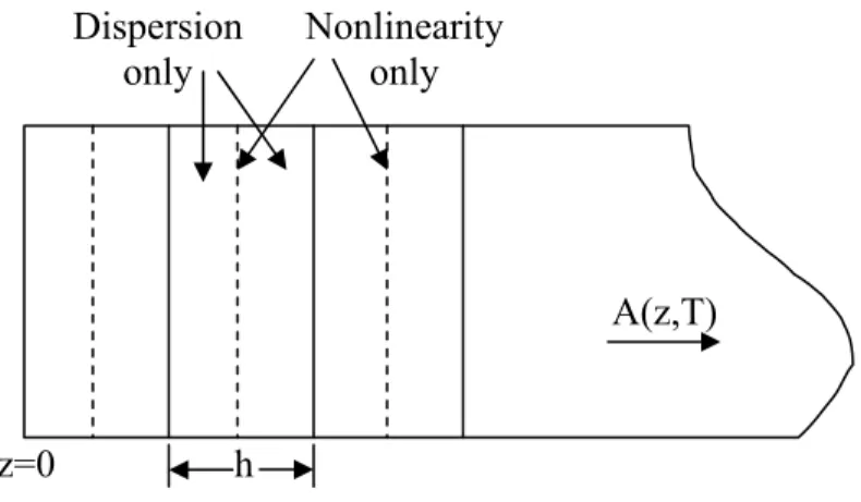
CHAPTER 4. LASER OSCILLATOR SYSTEM AND CHARACTERIZATION 47 The split-step Fourier method obtains an approximate solution by assuming that propagation over a small distance h is carried out in three steps. First, the pulse propagates over half the distance with only dispersive effects. Then, in the middle of the section, nonlinearity is included after which the pulse propagates again half the distance (Figure 4.1).

Figure 4.1. Illustration of split-step Fourier method used for numerical simulations

Mathematically,

, exp

2 exp exp 2 , 4.5

The exponential operators can be evaluated in the Fourier domain. For the dispersive operator exp , this yields

exp 2 , exp 2 , 4.6 Dispersion only Nonlinearity only A(z,T) z=0 h

(61)

where denotes the fourier transform operation, is obtained by replacing the differential operator / by . As is just a number in the Fourier space, the evaluation of Equation (4.6) is straightforward (see [18] for details).

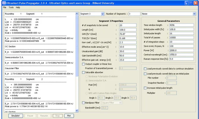
4.2.2. Simulator Interface

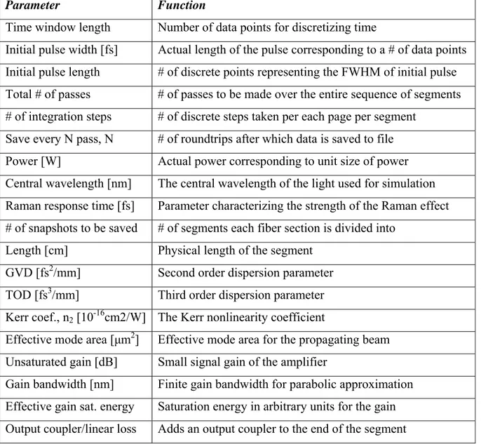
A screenshot of the simulator interface is shown in Figure 4.2. Table 4.1 summarizes the parameters needed for the numerics of the simulation.

(62)

CHAPTER 4. LASER OSCILLATOR SYSTEM AND CHARACTERIZATION 49 Parameter Function

Time window length Number of data points for discretizing time

Initial pulse width [fs] Actual length of the pulse corresponding to a # of data points Initial pulse length # of discrete points representing the FWHM of initial pulse Total # of passes # of passes to be made over the entire sequence of segments # of integration steps # of discrete steps taken per each page per segment

Save every N pass, N # of roundtrips after which data is saved to file Power [W] Actual power corresponding to unit size of power Central wavelength [nm] The central wavelength of the light used for simulation Raman response time [fs] Parameter characterizing the strength of the Raman effect # of snapshots to be saved # of segments each fiber section is divided into

Length [cm] Physical length of the segment GVD [fs2/mm] Second order dispersion parameter TOD [fs3/mm] Third order dispersion parameter Kerr coef., n2 [10-16cm2/W] The Kerr nonlinearity coefficient

Effective mode area [μm2] Effective mode area for the propagating beam Unsaturated gain [dB] Small signal gain of the amplifier

Gain bandwidth [nm] Finite gain bandwidth for parabolic approximation Effective gain sat. energy Saturation energy in arbitrary units for the gain Output coupler/linear loss Adds an output coupler to the end of the segment

(63)

The initial pulse shape can be one of the pre-defined pulse shapes ranging from Gaussian pulse shape to noise. Each segment of the laser should be configured separately. The saturable absorber is implemented at the end of a segment, by converting the total nonlinear phase shift accumulated over the round trip into an amplitude modulation. The semiconductor saturable absorber is modeled as;

1

1 4.7

where is the modulation depth and is the saturation power of the saturable absorber. For nonlinear polarization evolution, the model is;

1 cos

2 4.8

4.2.3. Simulation Results

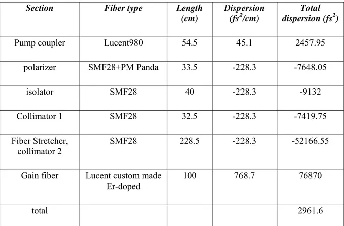
Simulation of the laser is done with the parameters summarized in Table 4.2. A total of six segments are required for the actual imitation of the laser. However, number of segments severely increases processor usage. For practical purposes, laser is simulated after some approximations resulting in just three segments instead of six segments. This approximation and %5 uncertainty associated with fiber properties (mode-field diameter, core diameter, numerical aperture, etc.) caused minor mismatch in simulated and experimental results. The output coupler section of the simulation is approximated as the total loss due to %5 tap port at isolator in addition to the loss at the NPE output. Although NPE, output coupler and interference filter are separated by single mode fibers, they were

(64)

CHAPTER 4. LASER OSCILLATOR SYSTEM AND CHARACTERIZATION 51 all assumed to be located at the end of first segment. Second- and third-order dispersion has been calculated from the data available in the component datasheets as dispersion depends linearly on core diameter and numerical aperture. There is no option for backward or forward pumping in the simulation, so any possible effect of backward pumping (experimental case) is not accounted for in the simulation results. Initial pulse is selected as noise for testing the simulation results. The numerical accuracy is also verified by checking that results are unaffected after doubling the sampling resolution.

Section Fiber type Length

(cm)

Dispersion (fs2/cm)

Total dispersion (fs2)

Pump coupler Lucent980 54.5 45.1 2457.95

polarizer SMF28+PM Panda 33.5 -228.3 -7648.05 isolator SMF28 40 -228.3 -9132 Collimator 1 SMF28 32.5 -228.3 -7419.75 Fiber Stretcher, collimator 2 SMF28 228.5 -228.3 -52166.55

Gain fiber Lucent custom made Er-doped

100 768.7 76870

total 2961.6

(65)

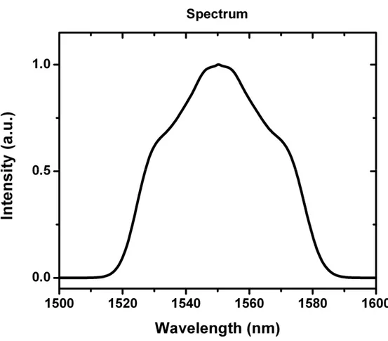
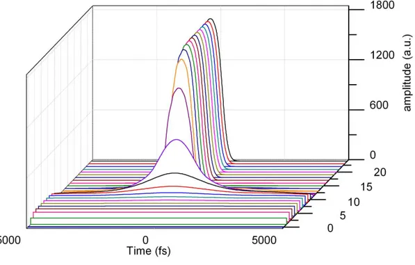
Figure 4.3 shows spectrum of the mode-locked laser which is a stable solution after 4500 roundtrips. In fact, laser can reach mode-lock state after around 50 roundtrips, but for the sake of stability check, pulse is rotated inside the cavity for 4500 roundtrips to achieve convergence to the last digit of the solution. Figure 4.4 shows buildup of the pulse from noise after 50 roundtrips.

(66)

CHAPTER 4. LASER OSCILLATOR SYSTEM AND CHARACTERIZATION 53