A newsvendor approach to energy imbalance mechanism in a day ahead electricity market

A NEWSVENDOR APPROACH TO ENERGY

IMBALANCE MECHANISM IN A DAY

AHEAD ELECTRICITY MARKET

a thesis submitted to

the graduate school of engineering and science

of bilkent university

in partial fulfillment of the requirements for

the degree of

master of science

in

industrial engineering

By

Ece C

¸ i˘

gdem

A NEWSVENDOR APPROACH TO ENERGY IMBALANCE MECHANISM IN A DAY AHEAD ELECTRICITY MARKET

By Ece C¸ i˘gdem June 2017

We certify that we have read this thesis and that in our opinion it is fully adequate, in scope and in quality, as a thesis for the degree of Master of Science.

Ay¸se Selin Kocaman (Advisor)

Kemal G¨oler(Co-Advisor)

Alper S¸en

¨

Ozgen Karaer

Approved for the Graduate School of Engineering and Science:

Ezhan Kara¸san

ABSTRACT

A NEWSVENDOR APPROACH TO ENERGY

IMBALANCE MECHANISM IN A DAY AHEAD

ELECTRICITY MARKET

Ece C¸ i˘gdem

M.S. in Industrial Engineering Advisor: Ay¸se Selin Kocaman

Co-Advisor: Kemal G¨oler June 2017

We study an energy imbalance problem in a day ahead electricity market from the perspective of a distribution company. This company commits to buy a cer-tain amount of electricity in the day ahead market the day before the actual demand of its customers is realized and faces energy imbalance due to demand uncertainty. This energy imbalance of the distribution company is penalized by a mechanism which includes penalty parameters defined by energy market reg-ulatory authorities. By developing a variant of the newsvendor model, we find the optimal commitment amount of the distribution company and analyze the effect of penalty parameters on this amount. We show that the way that penalty parameters are selected in current practice may lead the distribution company to underbid. With an empirical analysis performed on real data, we also show that effect of these penalty parameters could differ hourly, daily, seasonally, regionally and according to sectoral demand profiles. Considering that the traditional policy used to decide on the penalty parameters does not have a systematic approach, in this paper, we present insights for distribution companies on the optimal com-mitment decision as well as for the energy market regulatory authorities on how to choose the penalty parameters.

Keywords: day ahead electricity market, balancing market, power distribution company, newsvendor model, imbalance mechanism, penalty parameters.

¨

OZET

G ¨

UN ¨

ONCES˙I ELEKTR˙IK P˙IYASASI DENGES˙IZL˙IK

MEKAN˙IZMASINA GAZETEC˙I C

¸ OCUK YAKLAS

¸IMI

Ece C¸ i˘gdem

End¨ustri M¨uhendisli˘gi, Y¨uksek Lisans Tez Danı¸smanı: Ay¸se Selin Kocaman

E¸s-Tez Danı¸smanı: Kemal G¨oler Haziran 2017

Bu ¸calı¸smada, G¨un ¨Oncesi Elektrik Piyasası’ndaki bir da˘gıtım ¸sirketinin kar¸sıla¸stı˘gı enerji dengesizli˘gi problemi incelenmi¸stir. G¨un ¨Oncesi Elektrik Piyasası’ndaki da˘gıtım ¸sirketi, market i¸ci t¨uketim miktarı ¨ong¨or¨ulerini yapıp ger¸cek t¨uketim bilgisi ortaya ¸cıkmadan ¨once bu miktarı piyasadan satın almakla y¨uk¨uml¨ud¨ur. Fakat, da˘gıtım ¸sirketi sistemdeki talep belirsizli˘gi y¨uz¨unden enerji dengesizli˘gi ile kar¸sıla¸sabilir. Da˘gıtım ¸sirketinin kar¸sıla¸sabilece˘gı bu enerji den-gesizli˘gi, Enerji Piyasası D¨uzenleme Kurumu tarafından belirlenen ceza parame-trelerini i¸ceren bir ceza mekanizması ile cezalandırılır. Bu durum g¨oz ¨on¨une alınarak, bu ¸calı¸smada, ”Gazeteci C¸ ocuk” probleminin varyantı olan bir model ¨

onerilerek, da˘gıtım ¸sirketinin karını y¨ukseltmek i¸cin markete bildirilecek en iyi en-erji miktarının bulunması hedeflenmi¸s ve ceza paremetrelerinin bu miktara olan etkisi incelenmi¸stir. ˙Inceleme sonucunda, ceza parametrelerinin ¸su anki se¸cilme y¨onteminin, da˘gıtım ¸sirketinin ¨ong¨ord¨u˘g¨u enerji miktarından daha azını markete sunmalarına yol a¸ctı˘gı g¨osterilmi¸stir. Ayrıca, ger¸cek veriler kullanılarak, ceza parametrelerinin etkisinin saate, g¨une, sezona, b¨olgelere ve sekt¨orel talep profiller-ine g¨ore de˘gi¸siklik g¨osterdi˘gi bulunmu¸stur. Ceza parametrelerinin se¸cimi i¸cin kul-lanılan mevcut y¨onteminin herhangi bir sistematik yakla¸sıma dayandırılmamasını g¨oz ¨on¨unde bulundurarak, da˘gıtım ¸sirketlerinin en iyi talep tahmini kararlarını markete sunmalarına ve aynı zamanda Enerji Piyasaları D¨uzenleme Kurumu’na ceza parametrelerinin nasıl se¸cilmesi gerekti˘gine dair ¨ong¨or¨uler sunulmaktadır.

Anahtar s¨ozc¨ukler : g¨un ¨oncesi elektrik piyasası, dengeleme piyasası, da˘gıtım ¸sirketi, gazeteci ¸cocuk problemi, dengeleme mekanizması, ceza parametreleri.

Acknowledgement

I would like to express my sincere gratitude to my advisor Assist. Prof. Ay¸se Selin Kocaman and my co-advisor Assoc. Prof. Kemal G¨oler for all their support, guidance, understanding and help throughout this research and preparing me for the PhD journey.

I especially would like to thank Ay¸se Selin Kocaman for believing in me during my study. Not only she guided me on my thesis, but also she supported me in various ways with her friendliness. I consider myself lucky to have had the opportunity to work with her.

I also would like to thank Assoc. Prof. Alper S¸en and Assist. Prof. ¨Ozgen Karaer for accepting to read and review my thesis and their beneficial comments. I would also like to express my sincere thanks to B¨u¸sra ¨Okten who has sup-ported me during my study. Especially and most importantly, I would like to thank O˘guz Kaan Karakoyun for always being there for me. His efforts enabled me to achieve all my accomplishments.

Above all, I am deeply grateful to my mother Sevil Mete and my uncle Edip Sebahattin Mete, my aunt Sevgi Talas, my grandmother Mesrure Mete and my brother in law Aziz Talas for their endless support, patience and love throughout my life. They are my main motivation and always has been. It is important for me to feel that they are always proud of me.

Contents

1 Introduction 1

2 Literature Review 13

2.1 The Day Ahead Market . . . 13 2.1.1 Forecasting Techniques for Finding Optimal Electricity

Price in the Day Ahead Market . . . 14 2.1.2 Optimization Models for Finding Optimal Electricity Price

in the Day Ahead Market with Considering Non-Convexity of the Problem . . . 15 2.1.3 Optimal Bidding/Commitment Strategies in the Day

Ahead Market . . . 16 2.2 The Classical Newsvendor Model and its Applications in

Electric-ity Market . . . 21

3 A Newsvendor Model and Analysis 25 3.1 Analysis of the Model . . . 28

CONTENTS viii

3.2 Analysis of a special case: Uniformly-distributed realized demand

with linear supply function . . . 29

3.2.1 Standard uniformly distributed realized demand with linear supply function . . . 31

4 An application: Empirical calibration with real data 36 4.1 Hourly Analysis . . . 39

4.2 Daily Analysis . . . 42

4.3 Seasonal Analysis . . . 43

4.4 Regional Demand Analysis . . . 43

4.5 Sectoral Demand Analysis . . . 44

5 Conclusion 53

A Proofs of the Analytical Results 61

List of Figures

1.1 Illustration of bids of the market participants . . . 6 1.2 An example of a supply and demand curve where the equilibrium

point represents the market clearing price . . . 7 1.3 The process of the day ahead market and the balancing power market 9

3.1 The change in optimal commitment value with respect to penalty parameters k and l, where Y ∼ U (0, 1). . . 33 3.2 k and l combinations for different optimal commitment values

where k, l ∈ [0, 1] and Y ∼ U (0, 1) . . . 34 3.3 k and l combinations for different optimal commitment values

where k, l ∈ [−2, 2] and Y ∼ U (0, 1) . . . 35

4.1 Consumption amounts of the households of Baskent Distribution Inc. for the dates of January 2, 2014 and June 2, 2014 with respect to time. . . 38 4.2 Consumption amounts of the households and industries for

LIST OF FIGURES x

4.3 Consumption amounts of the households of Baskent and Bogazici Distribution Inc. in June 2, 2014 with respect to time. . . 39 4.4 The histogram and empirical distribution function of 1 a.m. . . . 45 4.5 The histogram and empirical distribution function of 8 a.m. . . . 46 4.6 The optimal commitment value x∗ for each hour with respect to

penalty parameters k and l . . . 47 4.7 The optimal commitment value x∗ for a peak (1 a.m.) and off-peak

hour (8 a.m.) with respect to penalty parameters k and l . . . 48 4.8 The optimal commitment value x∗for weekends and weekdays with

respect to penalty parameters k and l . . . 49 4.9 The optimal commitment value x∗ for different seasons with

re-spect to penalty parameters k and l . . . 50 4.10 The optimal commitment value x∗for Central Anatolia Region and

Marmara Region. . . 51 4.11 The optimal commitment value x∗ for different sectoral demand

profiles with respect to penalty parameters k and l . . . 52

B.1 The histogram and empirical distribution function of weekday . . 68 B.2 The histogram and empirical distribution function of weekend . . 69 B.3 The histogram and empirical distribution function of summer season 70 B.4 The histogram and empirical distribution function of winter season 71 B.5 The histogram and empirical distribution function of spring season 72 B.6 The histogram and empirical distribution function of fall season . 73

LIST OF FIGURES xi

B.7 The histogram and empirical distribution function of Baskent dis-tribution region . . . 74 B.8 The histogram and empirical distribution function of Bogazici

dis-tribution region . . . 75 B.9 The histogram and empirical distribution function of household . 76 B.10 The histogram and empirical distribution function of industrial . . 77

List of Tables

1.1 An example for single bids . . . 4 1.2 An example for block bids . . . 4 1.3 An example for flexible bids . . . 5

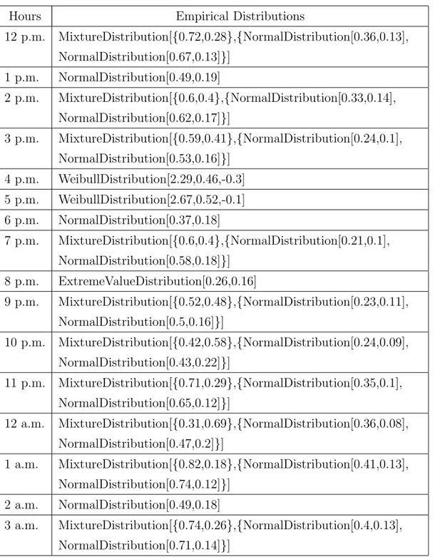
4.1 Empirical distributions for the hours between 12 p.m. and 11 a.m. of the household demand data for the months between September 2013 and August 2014 for Baskent Distribution Inc. . . 41

Chapter 1

Introduction

Historically, the electricity market structure was based on vertically integrated monopolies. Rather than being operated independently, electricity generation, transmission and distribution systems were operated from a single source. This market structure led lack of competition among companies, resulted with high operating costs, high retail prices and low supply security [1]. In order to over-come these inefficiencies, liberalization process started in the electricity sector in the late 1990’s [2]. With the emerge of liberalization process, electricity has be-come a tradable commodity. Trading electricity is, however, a challenging task. With having limited storability and transportability, electricity differs from other commodities and requires continuous balancing of demand (usage) and supply (generation). Over the past years, several trading mechanisms have been put into operations with this purpose. Goals of these mechanisms usually are to make the transactions between buyers and sellers easier, provide a safe balancing and settlement service, increase competition and hence provide a reliable mar-ketplace.

Day ahead markets can be considered as the backbone of the most liberalized electricity markets as the prices (market clearing prices) determined in this market are also used as reference points in other electricity markets and contracts [3]. By giving market participants a chance to purchase and sell energy for the next

day, the day ahead market aims to ensure that production and/or consumption needs and contractual obligations of them can be balanced one day ahead of the actual transfer. With this opportunity, if market participants could not sign a bilateral contract for trading electricity, they have another chance to trade.

Two main models are used while designing day ahead markets: Pool Models and European Exchange Models. In Pool Models, suppliers provide price contin-gent generation capacities (price-quantity bids) to the operator, however, demand is estimated by the system operator; meaning that distribution companies do not submit any demand bids. Based on the submitted bids by suppliers, and the esti-mated demand information, the system operator calculates the hourly electricity price of the market. In Pool model, as all physical transaction in the market is performed by the system operator, the transmission and generation coordination can be accomplished easily. Also, since the system operator realizes all dispatch in the market, the utilization of all resources can be increased if suppliers report their cost information accurately [4]. However, as suppliers are independent pri-vate power producers, they can reflect their cost structure untruthfully. If this situation occurs, because the demand side of the market does not have much contribution to the determination of prices, the calculated electricity price may be deceptive. Therefore, one can see that the Pool Model is vulnerable to the ma-nipulations by the supply side. Because of the reasons that are discussed above, many states of USA changed their market model from Pool Model to European Exchange Model, especially after California had suffered from the electricity crisis in 2000 [4].

European based day ahead markets use an exchange model where the genera-tion and distribugenera-tion companies both submit their bids to sell and buy electricity. Therefore, different than the Pool Model, the demand side participation is active in European Exchange Model, hence both sides of the market have contribution on determining the price of electricity. Suppliers can offer their electricity and buyers can purchase electricity either short or long term contracts in bilateral market. However, an appropriate supplier (buyer) may not always exist for a buyer (supplier) to make a contract or suppliers may not always sell their de-sired amount and buyers may not buy their needed amount of electricity with

contracts. In order to cope with this situation, day ahead market with European Exchange Model takes place for presenting suppliers and buyers another chance to trade electricity. With this chance, buyers can bid in order to compensate their energy deficit, whereas suppliers can bid for their unused capacity. Hence, the market price is determined with both buyers’ and sellers’ committed bids.

In this thesis, we are referring to the current Turkish day ahead market which adopts European exchange model for its operations [5]. The day ahead market is the main area in which purchase and sale transaction of electricity is traded one day ahead of the actual transfer of energy. In order to enable the market to operate without any disruption, the market operator and system operator play an important role. The main responsibility of the market operator is to manage the day ahead market and settlement activities of the market with transparency and accountability by balancing supply and demand. It is also responsible for informing market participants about transmission capacity of the grids, collecting and evaluating participants’ bids, and thereby calculating the market clearing price. After the market clearing price and dispatch amount are finalized, the market operator has to deliver this information to the participants and evaluate the objections that come from them.

The system operator ensures instantaneous balance of the actual and commit-ted purchases and sales while conserving supply quality [6]. It has to calculate the transmission capacity of grids and inform the market operator before the day ahead market starts. Moreover, in the real time operations, the system opera-tor checks the feasibility of dispatchings and calculate the system marginal price in the balancing power market in order to balance supply and demand. In the Turkish Day Ahead Market, Market Financial Settlement Center (MFSC) and National Load Dispatch Center (NLDC) which are both under the body of Turk-ish Electricity Transmission Company (TEIAS) are the market operator and the system operator, respectively [6].

The day ahead market transactions are performed every day on hourly basis. Transactions in each day starts at 12:00 p.m. and ends at 12:00 p.m. next day. Hence, the submission of the bids has to end one day before the actual transfer of

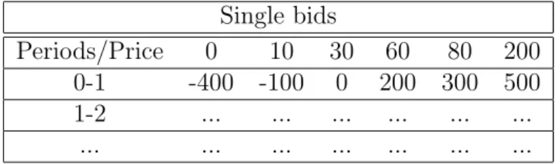
Table 1.1: An example for single bids Single bids Periods/Price 0 10 30 60 80 200 0-1 -400 -100 0 200 300 500 1-2 ... ... ... ... ... ... ... ... ... ... ... ... ...

Table 1.2: An example for block bids

Block bids

Periods Price Quantity 0-6 100 100 12-24 35 -30

energy. Market participants submit their bids for every hour in a 24-hour period. The submitted bids should consist of a certain time period (hour), quantity in MW (production or demand quantity), and price in TL/MW. Each bid that consists of price and quantity pairs may differ hourly. There are three types of bids that can be submitted in the day ahead market such as single bids, block bids and flexible bids. Single bids that include price and quantity schedules are traded for a particular period of the next day. Table 1.1 demonstrates a single bid for the first hour. For example, the bidder is ready to sell 300 MWh if the market clearing price is greater than or equal to 80 TL/MWh and ready to buy 100 MWh if the market clearing price is less than or equal to 10 TL/MWh. In block bids, participants can submit block selling or buying bids for more than one successive time periods. However, contrary to single bids, they can not submit a selling and buying bid for the same time period. For instance, in Table 1.2, the bidder is ready to sell 100 MWh for each period of 0 to 6 if average market clearing price is greater than 100 TL/MWh and willing to buy 30 MWh for the periods of 12 to 24 unless the average market clearing price is greater than 35 TL/MWh. The block bids can be used in the case where the production is continuous and the cost of starting and stoping a power plant is high [5]. In flexible bids, there are single hour sale or purchase bids that are not restricted for a certain period or

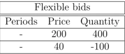
Table 1.3: An example for flexible bids

Flexible bids

Periods Price Quantity - 200 400 - 40 -100

periods. The quantity and price schedule that market participants submitted is valid for each time period. In Table 1.3, in the first flexible bid, the bidder is willing the sell 400 MWh if the maximum market clearing price is greater than 200 TL/MWh and in second bid, he/she is ready to buy 100 MWh if minimum market clearing price is smaller than 40 TL/MWh.

Market operator informs market participants at 9:30 a.m. about the hourly available transmission capacity of the grid which is determined by the system operator. By 11:30 a.m, market participants submit their bids to the market operator. Each submitted bid is accepted or rejected by the market operator until 12:00 p.m. Any bid that does not satisfy the collateral liabilities of the market participants is rejected. In addition to that, each total sale and purchase quantity amount submitted to day ahead market should not exceed the limits determined by the market operator. To balance the supply and demand, all accepted hourly selling bids and their corresponding quantities are listed increasingly starting from the lowest price and its corresponding quantity value and all submitted hourly buying bids and their corresponding quantities are listed decreasingly starting from the highest price by the market operator. Those bids are inserted to the supply-demand curve in which hourly selling bids constitute supply and hourly buying bids constitute demand curve. The intersection of these curves is the point where there is no surplus or shortage of electricity for the market; meaning that the system is in equilibrium. The point calculated by the market operator between 11:30 a.m. and 1:00 p.m. is the next day’s day ahead market price (market clearing price). Since demand and supply bids are differed for each hour, market clearing price is calculated on hourly basis, thus, each hourly period has different market clearing price.

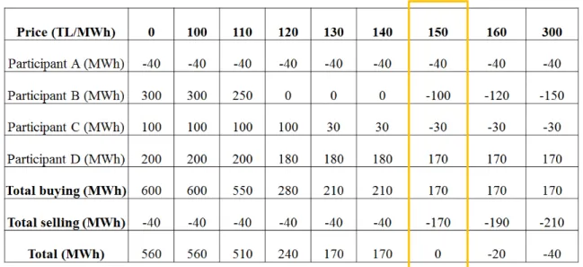
Figure 1.1: Illustration of bids of the market participants

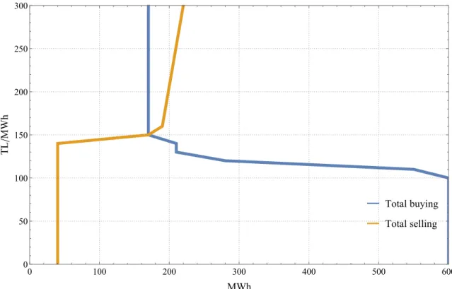
Figure 1.1 illustrates the bids of 4 participants to the day ahead market. All prices are listed from lowest to the highest price (- denotes bids for selling and + denotes bids for buying electricity). Selling bids of each participant constitute the supply curve and buying bids of each participant constitute the demand curve. In total, for each price value, electricity amounts for each price value are added to each other. The point where 0 occurs represents the equilibrium point where buying quantity is equal to selling quantity. Combined supply demand curve using interpolation method is shown in Figure 1.2. Figure 1.2 shows that the equilibrium point which gives the market clearing price is obtained at 150 TL/MWh with the amount of 170 MWh of electricity. Hence, 170 MWh of electricity has to be produced as well as consumed at the specific time period in the day ahead market.

Total buying Total selling 0 100 200 300 400 500 600 0 50 100 150 200 250 300 MWh TL /MWh

Figure 1.2: An example of a supply and demand curve where the equilibrium point represents the market clearing price

After market clearing price is calculated, the approved buying and selling quan-tities and prices that are valid for the next day are announced by the market operator. For example, for the bids that are shown in Figure 1.1, the resultant day ahead market dispatching is as follows;

Participant A will sell 40 MWh energy Participant B will sell 100 MWh energy Participant C will sell 30 MWh energy Participant D will buy 170 MWh energy

After related dispatching is announced to the market participants, they have a right to object to the tradings between 1:00 p.m and 1:30 p.m. The objections are evaluated by the market operator till 2:00 p.m. and the final trading is determined. Hence, the energy trading is completed one day before the actual

transmission. The process of the day ahead market can be seen in Figure 1.3. In the day ahead market, participants are encouraged to submit their best predictions about their generation or demand amounts to minimize the difference between actual purchases or sales as a result of real-time balancing of supply and demand. This difference between scheduled generation (or usage) and the actual generation (or usage) is called the energy imbalance and managed in the balancing power market. In the balancing power market, market participants submit their offers/bids (the difference between the realized and committed amounts) till 4:00 p.m. to the system operator. These offer and bid volumes are lined up according to the price for every hour. After 5:00 p.m, in order to prevent the falling to the imbalance in the system, the submitted offer volumes and bid volumes are balanced and a reference price (system marginal price) is calculated by the system operator. Imbalance in the system can be seen in two ways such as energy deficit and excess energy. System marginal price is determined as the maximum hourly offer price in the case of energy deficit and the minimum hourly bid price in the case of excess energy. The process of the balancing power market can also be seen in Figure 1.3.

In the electricity market, demand and supply must be in equilibrium at all times since if not, the energy imbalance may cause degradation of the whole power system, or even black out. Therefore, in the Turkish day ahead market, market participants who experience energy imbalance in the market are penalized by a double price mechanism in which the penalty is based on both the system marginal price (SM Pt), market clearing price (M CPt), and penalty parameters (k and l)

according to the 111th _{article of Electricity Market Balancing and Settlement}

Regulation given below:

EIPt = EIVt(−)max(M CPt, SM Pt)(1 + k) + EIVt(+)min(M CPt, SM Pt)(1 − l)

(1.1) The energy imbalance penalty (EIPt) consists of the positive and negative

Figure 1.3: The pro cess of the da y ahea d mark et and the ba lancing p o w er mark et

system marginal price (SM Pt) at settlement period t and penalty parameters (k

and l). This pricing mechanism guarantees that if the market participant has an excess of energy, this energy is sold with a price which is less than or equal to the minimum of SMP and MCP. Likewise, if the market participant has a deficit of energy, the company buys the energy with a price which greater than or equal to the maximum of SMP and MCP. With this mechanism, participants are punished both when they make an overcommitment and an undercommitment. How much the price will differ from the minimum (maximum) of SMP and MCP in case of overage (underage) depends on the penalty parameter l (k).

In Turkey, market participants were penalized with the unit prices used in undercommitment (maximum of M CPt and SM Pt) and overcommitment

(min-imum of M CPt and SM Pt) before 2013. However, in this pricing mechanism,

there were situations in which market participants were able to avoid to commit their true forecasts. According to Annual Report of Energy Market Regulatory Authority of Turkey in 2013, to fix these situations, the penalty mechanism for energy imbalance has changed on 5th of January, 2013 [7]. New penalty param-eters are defined as the coefficient in the case of undercommitment (k) and the coefficient in the case of overcommitment (l) are implemented in the energy im-balance penalty mechanism. They are defined between 0 and 1 (k, l ∈ [0, 1]), and they are both 0.3 for the time being in 2017 [7]. The reason why these penalty parameters are included in the energy imbalance payment is to force the company to make accurate predictions about their generation or consumption and report their true forecast information and reduce overall imbalance rates. At this point, the question that comes to mind is how effective these parameters are to reduce the energy imbalance rate.

In this thesis, we analyze the selection policy of the penalty parameters while focusing on their effects on the optimal commitment of a distribution company. A distribution company in the market commits predictions of its customers’ con-sumption to the day ahead market in a day before the actual demand is realized. Those predictions are not always made accurately since the forecasts are generally based on seasonal conditions and system constraints. Moreover, the distribution company can make a false demand reporting deliberately in order to manipulate

the regulating price as the optimal amount which maximizes the profit of the company would be different than the forecasted amount because of the imbal-ance penalty mechanism. Therefore, the main aim of this study is to analyze the effectiveness of the selection policy of penalty parameters in this imbalance penalty mechanism by developing an analytical model. To examine this, we work in the day ahead market by assuming that there is a single distribution company who faces demand uncertainty and suppliers’ behaviors are exogenous and fixed in the market. Also, we assume the prices are determined based on monotoni-cally increasing supply functions. According to our assumptions, we develop a variant of the newsvendor model to analyze the distribution company’s optimal commitment amount in the day ahead market which maximizes its profit and to illustrate the impact of penalty parameters on this amount.

We show that without the penalty parameters, the distribution company has tendency to underbid. Choosing the penalty parameters equal to each other and between 0 and 1, as it is currently done, still leads the distribution company to underbid in the market and in order for the distribution companies to commit their actual predictions, the penalty parameters (k and l) should be chosen dif-ferently than the current practice. Moreover, we show that the time and season of the year and demand profiles for different regions and sectors are important factors that should be taken into account while choosing the penalty parameters. Characterizing the impact of the penalty parameters for energy imbalance pay-ments on the commitment amount both analytically and empirically using real data from Turkey, is the main contribution of this thesis. Considering that the traditional policy does not have a systematic approach on the selection process; in this study, we present insights for distribution companies on the optimal com-mitment decision as well as for the Energy Market Regulatory Authorities on how to choose the penalty parameters.

The rest of this thesis is organized as follows: In Chapter 2, we review the lit-erature of the day ahead electricity market and the classical newsvendor problem and its applications in electricity market. In Chapter 3, we present the overview of the proposed model and propose analyses of the model in order to discuss the behavior of a distribution company in the market and the efficiency of the

selection policy of penalty parameters. In Chapter 4, an empirical calibration and analysis are presented with real data in order to see the effect of time, re-gion, season and demand profiles on the penalty parameters. The final chapter, Chapter 5, includes the concluding remarks.

Chapter 2

Literature Review

In this chapter, we review the literature related to our work. We summarize the existing works under two subsections: (i) the day ahead market, and (ii) the classical newsvendor model and its applications in electricity market.

2.1

The Day Ahead Market

The day ahead market literature is divided in to two streams: finding optimal electricity prices in the market and finding optimal bidding/commitment strate-gies for the market participants.

The determination of the market clearing price in the day ahead market is im-portant since it helps companies to make their risk management in short term and long term. Market clearing price is used as a reference price by the participants to determine their future price and quantity bids. Finding optimal electricity prices in the day ahead market stream considers both forecasting the optimal prices from the historical data and modeling the day ahead problem of finding optimal prices in the case of non-convexities in the market.

2.1.1

Forecasting Techniques for Finding Optimal

Elec-tricity Price in the Day Ahead Market

In order to determine hourly market clearing price, several statistical forecasting methods are used. Generally, autoregressive (AR), moving average (MA), au-toregressive moving average (ARMA), auau-toregressive integrated moving average (ARIMA), and generalized autoregressive conditional heteroskedastic (GARCH) models are used as stochastic time series methods. Additionally, causal models (regression models) which take electricity price as a dependent variable and model it as a function of independent variables (e.g.demand) are presented. Since elec-tricity price has high volatility and nonlinearity, artificial neural network based models and data-mining models are also used as forecasting techniques. In addi-tion to all these models, optimizaaddi-tion models are also used in order to find the optimal electricity price in the day ahead market.

Cuaresma et al. [8] use univariate time series models (AR and ARMA) to predict hourly market clearing prices. They analyze the performance of those models by using the hourly data taken from German Leipzig Power Exchange (LPX). They find that hourly modeling improve the prediction accuracy of linear univariate time series models.

Garcia et al. [9] predict next day market clearing price by using GARCH model in which demand is taken as an exogenous variable. They make an empir-ical analysis using Spain and California electricity market data. Their proposed method gives a better forecast comparing to ARIMA model when there are price volatility and spikes.

Nogales et al. [10] use two techniques such as dynamic regression and transfer function models in order to forecast the next day electricity prices. They find that price forecasts obtained from their models provide accurate results for buyers and suppliers to prepare their bidding strategies. They also analyze Spain and California markets and observe that comparatively high volatility and dispersion are seen in the prices of Spain market.

Rodriguez and Anders [11], and Amjady [12] use neural network models to predict market clearing price. Their models differ from each other with respect to input variables, number of trained data and preprocessing techniques. However, they both claim that their proposed methods find better results than univariate time series models.

Yan et al. [13] propose support vector machine (SVM) approach in order to forecast electricity price. Since it is important to select efficient training param-eters for SVM in order to increase its performance, they use genetic algorithm to predict SVM parameters. The analysis, which is performed by using the elec-tricity price data of China, shows that proposed method has better prediction accuracy than artificial neural network algorithm.

2.1.2

Optimization Models for Finding Optimal

Electric-ity Price in the Day Ahead Market with Considering

Non-Convexity of the Problem

When market participants submit their bids, the day ahead market problem (finding clearing prices) is a convex optimization problem. If the strong duality holds in the problem, the dual variables of the problem can be regarded as optimal prices [14, 15, 16]. However, some orders (e.g. block orders) lead non-convexities in the optimization problem so finding market clearing price becomes an NP-Hard problem [5]. To deal with non-convexity, several mixed integer programming (MIP) formulation and solution approaches have been developed.

Ruiz et al. [16] propose a methodology that relies on finding an LP and its dual program by relaxing the integrality constraints of the MIP problem and minimize the duality gap between two LPs. Since they minimize the duality gap, the resulting prices can be taken as the optimal market clearing prices.

The solution time of the day ahead problem (finding optimal electricity prices) is important since the decrease in the solution time gives the market operator a

chance to examine the offers and related dispatching before announcing them to participants. Regarding this issue, Derinkuyu [5] develops an MIP model to find electricity prices in the Turkish day ahead market with less computational time. Their MIP formulation with aggregation and variable elimination techniques re-duce the MIP formulation size significantly. They also develop an Integer Pro-gramming based neighborhood heuristic to find an upper bound for the optimal value.

Additionally, in order to decrease the solution time of the day ahead problem, some exchanges restrict the block orders in the market. Meeus et al. [17] discuss the logic behind the restrictions against the block orders. Their mixed integer programming model includes the binary variables for both block and hourly bids. They find that on the contrary to the current belief, the restriction of the block orders may not decrease the solution time of the day ahead market problem.

Madani et al. [18] considers both block orders and piece-wise linear orders in their MIP model. They use strong duality theory for their quadratic optimization problem and propose a method which can be directly implemented in existing MIP solvers.

2.1.3

Optimal Bidding/Commitment Strategies in the

Day Ahead Market

In the day ahead market, all market participants are required to submit their commitments which show the amount of energy that they are willing to buy/sell in the market. Since participants aim is to increase their profits, their commitments in the day ahead market gains importance. Therefore, there are several studies on the optimal bidding/commitment strategies. These studies generally include the analysis of the commitment schedules of the supply side (generators) and/or the demand side (distributors) of the market by using optimization and/or game theory based models when supply and/or demand certain or uncertain.

2.1.3.1 Optimal Bidding/Commitment Strategies for the Supply Side of the Day Ahead Market

Song et al. [19] optimize the bidding decision of a single supplier in the centralized day ahead market by using stochastic optimization method. The competitors’ bids are constructed with the probability distributions that are obtained from the related historical market data. They find a robust solution to respective optimization problem. Also, they consider bidding under ”multiple commodity second price auction” mechanism. This mechanism pushes the company to bid at their marginal costs (their true cost information). They show that suppliers can increase their profits by bidding under this concept.

Conejo et al. [20] consider a price-taker producer and aim to find the opti-mal bidding schedule of this producer who faces with price uncertainty in the day ahead market. The electricity prices are determined as hourly random vari-ables which represent the prediction of the actual prices. They find an optimal commitment value by maximizing the producer’s profit. According to this value, they provide a bidding strategy. By verifying their model with multiple cases, they assert that their model is effective to solve the optimal bidding schedule of a price-taker producer.

Rodriguez and Anders [21] also propose a methodology for finding the optimal bids for a price-taker producer. They improve the method that is proposed in [20] to consider two types of participants which are risk averse and risk seeker. They model the uncertainty of price (scenario based) based on the predicted price and the forecast error revealed in the forecasting process. They built a bidding curve with several scenarios and propose several decisions like based on which blocks of the curve participants should submit for each hour.

Gountis et al. [22] propose a model with two level optimization problem in order to develop the optimal bidding strategies for producers. In the first level, the market participant maximizes its expected profit, and in the second level, the system operator solves an optimization problem in order to find the market prices and optimal dispatches. They assume that suppliers bids are built as linear

supply functions and suppliers commit their production schedules according to the estimated demand and their rivals’ behavior. They use Monte Carlo simulation to calculate the expected profit and a genetic algorithm to find optimal bidding strategies for suppliers.

Wen and David [23] highlight the importance of imperfect market where partic-ipants do not have information about their rivals’ bids. They affirm that suppliers in the perfectly competitive market is willing to bid close to their marginal pro-duction costs so as to increase their profits, yet in the imperfect market they may want to give higher bids compared to their marginal production costs. Given this point, they model the optimal bidding decision of suppliers by using stochastic optimization model. They assume that every supplier in the market bid a linear supply function and can choose the coefficients of their linear supply functions in order to maximize their gains. Constructing an example with six suppliers, they observe that the market clearing price is higher in the imperfect market when suppliers propose their bids strategically compared to the perfectly competitive market.

Baillo et al. [24] propose strategies for generation companies using mixed linear integer programming considering the effect of company’s bids on the price of electricity and the uncertainty that the company faces because of not knowing the behavior of other rivals.

Many studies in the literature about the day ahead market has disregarded the transmission congestion in their models. However, Peng et al. [25] model the optimal bidding strategy of suppliers by considering transmission congestion which can have an influence on the market clearing prices and hence the bidding strategies of the market participants. They model the bidding strategy of the supplier as a three level optimization problem including transmission congestion management and implement a game theory model to find the optimal bidding strategies of suppliers.

generation in a day ahead market that consist of finitely many competing com-panies in the presence of supply uncertainty. They define two different markets such as credit-dominated and penalty-dominated market in the day ahead market. Generators are penalized in penalty dominated market with the sum of undersup-ply and oversupundersup-ply penalty rate, whereas in credit-dominated market they have to pay an undersupply penalty and get an oversupply credit. Those penalty and credit rates are defined as linear functions of the market clearing price. Based on their market definition, they use the theory of ordinary differential equations in order to characterize each firm’s committed production schedule and respec-tive actual production volumes in the day ahead market with or without subsidy. They find that the oversupply and undersupply penalty rates have trivial ef-fects on the committed production schedules and actual production strategies of generators, and also on the market clearing price. They also prove that if un-dersupply penalty rate is imposed to the market, companies tend to overcommit their expected production quantity and lower market clearing price is observed.

2.1.3.2 Optimal Bidding/Commitment Strategies for the Demand Side of the Day Ahead Market

Liu et al. [27] consider energy service providers’ problem on purchase allocation and demand bidding in different markets with two objectives: the total cost and risk. They generate demand curves and market prices according to the real data taken from California market. The optimal purchase allocation is found by using stochastic modeling.

Fleten and Pettersen [28] propose a stochastic linear programming model for constructing piece-wise linear bidding curves that are submitted to the Nordic power exchange. They examine a price-taker buyer in the market. In their models, they consider the imbalance volumes that occur because of the difference between predicted and realized demand. The buyer is penalized with the unit prices of respective imbalance volumes. They find that there is a trade-off between the expected profit and expected penalty. Hence, they conclude that in order for a retailer to increase its expected profit, it should increase the difference between

its commitment amount and realized demand.

Philpott and Pettersen [29] present a model which includes a buyer and seller in Norway day ahead electricity market. The main aim of this study is to analyze the behavior of buyers (purchasers) in the day ahead market and thereby examine the market clearing price deviations. The first model that they present, consists of a single buyer in the market. They find that the optimal commitment amount of the buyer is its expected demand when all generators submits same prices in the market. However, when generators submit supply functions with a single price and its respective quantity, they find that the buyer bids less than its expected demand. In the second model, they examine the two-period game played between many purchasers and a single supplier in a competitive environment. In both models, they show that the day-ahead prices would be lower than the expected real-time prices as the purchasers have an incentive to underbid.

Herranz et al. [30] propose a genetic algorithm which solves the optimization problem of a buyer in order to find its optimal bidding value to achieve minimum purchase cost. The market structure that they defined is a combination of a day ahead market and an intra-day market. They present the effect of the participants on the market clearing price by residual supply curves in order to compute new clearing prices. They assume that the buyer sell the amount energy with minimum price and buy the amount of energy with maximum price in the market; meaning that prices in their model are chosen to be deterministic. The model is tested with the real Spanish day ahead market and intra-day market. They assert that the solution methodology is efficient, feasible and robust.

Kazempour et al. [31] propose a mathematical model and a heuristic approach for large consumers to develop bidding strategies to affect the prices for their own benefit. They find that a strategic consumer may commit at prices lower than of that will increase their marginal utility. Hence, the market clearing price decreases and expected utility of the consumer increases respectively.

buyers in the day ahead market. In addition, they propose a solution using mixed-linear integer programming for risk-averse buyers. They assume that the demand may change according to the price of electricity (price-dependent demand). They find that when the buyer is risk-neutral, they should give a single bid. However, when the buyer is risk-averse, block bidding curve provides more benefit to the buyer by mitigating the risk.

There are many studies that mainly base on finding optimal market clearing price and optimal bidding decisions for market participants. Studies that deal with the optimal bidding decisions generally approach to the problem for the supply side of the market. Thus, there is relatively less focus on the bidding strategies for demand side. Unlike the aforementioned studies, we characterize the impact of the penalty parameters for energy imbalance payments on the com-mitment amount both analytically and empirically using real data from Turkey. We also analyze the behavior of a distribution company in the presence of these penalty parameters.

2.2

The Classical Newsvendor Model and its

Applications in Electricity Market

The problem faced by a newsvendor is to decide how many newspapers to order before observing the real demand. The newsvendor faces overage or underage costs if he/she orders too much or too little. This famous operations research problem has also been studied in the literature for the operations in energy mar-kets.

Sethi et al. [33] aim to provide insights to the suppliers about their best bidding strategies. They study a market that consists of two suppliers and one buyer who uses the classical newsvendor solution as his/her forecasted demand. Since each supplier competes for the buyer’s purchase amount, a game theory environment occurs. Therefore, each supplier’s optimal bidding strategy is found

by using game theory approach. The suppliers’ bidding curves are accepted as linear functions. They show that the buyer benefits from the competition among suppliers since a lower market clearing price is observed. The proposed method is applied to the power generator plants in the California electricity market.

Kim and Powell [34] derive the closed form representation of the optimal en-ergy commitment policy for wind farms by using newsvendor model. With their proposed model, they are also able to make derivations about the value of storage and storage losses. Their optimal commitment policy model is based on heuristics and simulation models instead of stochastic optimization models. Their assump-tions about distribution of wind (uniform distribution) and size of the storage make their model easy to evaluate. However, in the real life, for more general cases about the distribution of the wind speed and energy storage, they assert that their analytical model may not work but they can use numerical results to calibrate their model.

Bitar et al. [35] use newsvendor model in order to find the optimal contract offerings and optimal expected profit of a wind power producer in the competitive market. In the profit function of their model, the producer is punished both for their overcommitment and undercommitment. Bitar et al. [35] assume that imbalance prices which are used in overcommitment and undercommitment case can take both positive and negative values, and the producer does not have energy storage option. Based on these assumptions, optimal contract offerings are found. They state that there is a trade-off between imbalance prices and the need for energy curtailment.

Densing [36] studies a price-driven dispatch planning problem by using newsvendor approach to decide when to sell or buy a certain amount of en-ergy in the first stage of their research. The dual of their primal optimization problem gives a newsvendor problem which turns the price-driven dispatch plan-ning to demand-driven dispatch planplan-ning. They find certain price thresholds that help the generation company to determine the amount that it should produce for a given price. In the second stage, they use multistage stochastic linear pro-gramming for high-frequency dispatch decisions, and test their model with a case

study.

Secomandi and Kekre [37] investigate the optimal policy for suppliers which is based on submitting their production amount partially in the forward market rather than submitting all of their production in the spot market. The aim of the study is to provide a balance between the costs that a supplier faces with in the spot market and in the forward market. In their study, the supplier can not store the energy, yet it can sell energy to the spot market. Also, it can sell energy partially by entering the forward market. How much energy to sell to the market is obtained by solving a generalized newsvendor problem. In the newsvendor model that they consider the demand as well as the spot price as uncertain variables.

Nair et al. [38] aim to search the effect of long term contracts on the bid-ding strategies of renewable energy generators (e.g. wind power producers) and how the optimal bidding strategy changes as the level of renewable penetration increases. They evaluate the optimal bidding strategy of a wind power pro-ducer who signs long term contracts with companies instead of participating in a competitive electricity market. They use a variant of the classical newsvendor model by substituting demand with residual demand (thereby making demand uncertain). Using the price as a shortfall penalty, they compute a closed form solution for the optimal energy commitment value. Moreover, they change the market structure by adding new intermediate market (forward market). It turns out that adding an intermediate market will decrease the average cost of sell-ing energy, however, the change in total amount of conventional energy is based on the distribution of the difference between wind estimate and the actual wind realization.

Aflaki and Netessine [39] investigate the link between the intermittency of renewable energy sources and the effectiveness of promoting policies for renew-able sources such as carbon pricing. They use the classical newsvendor model to find the optimal capacity to be invested in the long term contracts. They show that charging more for emissions resulting from nonrenewable sources can unexpectedly discourage investment in renewables.

Wan and Fan [40] develop two-stage method on newsvendor problem for strate-gic purchasers in the day ahead market and real-time market. In the first stage of the proposed method, the purchaser commits to buy a certain amount and makes another commitment in the second stage. The prices are chosen to be deterministic and not dependent on the commitment size. The model decides on the optimal commitment amount in the first and second stage.

Based on our analysis of the day ahead market and newsvendor model used in electricity market literature, to the best of our knowledge, there is no study that considers the effect of penalty parameters on distribution companies’ commitment strategies and the selection policy of penalty parameters used in the Turkish day ahead market by using a newsvendor model. This thesis aims to contribute the literature by providing an analytical approach to the market on the selection policy of the penalty parameters which plays an important role on the energy imbalance volume and by providing a discussion on the behavior of distribution companies in such a penalty mechanism.

Chapter 3

A Newsvendor Model and

Analysis

The main aim of the day ahead market is to balance supply and demand for the following day. In a European exchange type day ahead market that we study in this thesis, a buyer (a distribution company) submits the desired amount of energy to be purchased based on the forecasted demand of the customers for each hour on the next day; whereas a seller (a generation company) submits the amount of energy that is planned to sell for each hour on the next day. In our model, we consider a distribution company who faces demand uncertainty in the day ahead market.

Consider a day ahead market with a single distribution company that has commitment amount (also assumed to be the cleared demand bid amount) x. The distribution company’s decision process is based on the newsvendor problem that divides its decision process into two stages. In the first stage, the day ahead market is run and the distribution company has to decide its commitment amount which will determine the market clearing price. We assume that the behaviors of the suppliers are exogenous and fixed with a supply curve S(·). With perfect knowledge of S(·), which is a monotonically increasing supply function, the distribution company can decide on the commitment amount x and chooses

any decreasing demand curve that passes through (x, S(x)). The point (x, S(x)) represents the company’s commitment (i.e. the company is willing to buy x amount of electricity with a price of S(x)). Therefore, the market clearing price is determined as S(x) in our market structure.

The second stage of the newsvendor model consists of the real time operations of the market. The realized energy amount in the real time is defined as a random variable Y , with a mean µY > 0, a differentiable cumulative distribution function

F (·) and density function f (·) > 0 on support R+_{. Based on the energy deficit or}

surplus observed after the actual demand is realized, the distribution company makes a new commitment to buy or sell the amount of energy according to the dif-ference between realized demand and the committed amount that was determined in the first stage. When the actual demand is realized, the point which represents the realized demand (Y ) in the supply function determines the system marginal price. In Philpott and Pettersen [29], the system marginal price is taken as the market clearing price plus another supply function (e.g. δ(·)) that denotes the difference between the system marginal price and the market clearing price (e.g. S(x) + δ(Y − x)), whereas Fleten and Pettersen [28] represent system marginal price with a constant parameter. Hence, there are several representations of the system marginal price. Here, since we assume that the supply function is fixed in the model, the system marginal price is also defined by the monotonically in-creasing supply function S(·). This implies that the system marginal price which is determined as S(Y ) and market clearing price S(x) are specified based on the same supply function. Note that, since Y is a random variable, system marginal price is also a random variable.

The total imbalance payoff formula given in equation (1.1) is revised according to our model by writing (Y − x) instead of negative imbalance amount EIVt(−),

(x − Y ) instead of positive imbalance amount EIVt(+), S(x) instead of M CPt,

and S(Y ) instead of SM Pt according to the assumptions that are given above.

The revised formula is given below:

The energy imbalance volume is reflected to the distribution company as a cost in the case of their commitment amount is different than the realized demand. The profit of the distribution company during a single time-slot is driven as a variant of the newsvendor model since the distribution company commits the forecasted amount to the market; meaning that it gives an order, and in the case of overcommitment or undercommitment (overforecast or underforecast), it has to pay an overage or underage costs with respect to the difference of realized and committed demand. Hence, the profit function of the distribution company is given below: Π(x, Y ) =    pY − S(x)x − (Y − x)max[S(x), S(Y )](1 + k) if x < Y pY − S(x)x + (x − Y )min[S(x), S(Y )](1 − l) if x ≥ Y (3.2)

According to the model, the distribution company sells Y with the retail price p ∈ R+ _{to the customers in the actual day. It buys x from the market with the}

market clearing price S(x) the day before the actual demand is realized. Ac-cording to its commitment value x, it has to pay a negative energy imbalance payment (underage cost), (Y − x)max[S(x), S(Y )](1 + k), if it commits less than the realized demand. On the other hand, it has to pay an positive energy imbal-ance payment (overage cost), (x − Y )min[S(x), S(Y )](1 − l), if it commits more than the realized demand. The imbalance price in the case of undercommitment is given as max[S(x), S(Y )] and as min[S(x), S(Y )] in the case of overcommitment. The term (1 + k) causes to increase the loss of the company and (1 − l) causes the company to make less profit than they should make otherwise. In total, the company has revenue from selling the actual demand to the customers, costs from buying, loss from selling in the day ahead market and cost from creating energy imbalance in the system by failing to meet the commitment. Therefore, while deciding on the amount of energy to purchase in the day ahead market, the de-cision must incorporate the imbalance prices max[S(x), S(Y )], min[S(x), S(Y )] and also the penalty parameters k and l.

x, that maximizes the expected profit given below:

E[Π(x, Y )] = Z x

0

(py − S(x)x + (x − y)S(y)(1 − l))f (y)dy +

Z +∞

x

(py − S(x)x − (y − x)S(y)(1 + k))f (y)dy (3.3)

Using the general formula given in 3.2, after the optimal commitment amount that maximizes equation 3.3 is found, the behavior of the distribution company in the market with and without penalty parameters and the efficiency of the current selection policy of the penalty parameters are analyzed in this chapter. Also using the formula 3.3 again, the effect of the time of the year, region and demand profiles on the penalty parameters are discussed in Chapter 4.

3.1

Analysis of the Model

Proposition 1 below proves the existence of a closed form solution for the optimal commitment value x∗.

Proposition 1. The value of x that solves S(x)+xS0(x)+(k+l)R₀xS(y)f (y)dy = (1 + k)µS(Y ) is the optimal solution to the following maximization problem:

max

x≥0 pµY − S(x)x + (1 + k)(xµS(Y )− µS(Y )Y) − (k + l)

Z x

0

(x − y)S(y)f (y)dy (3.4)

Proof. See Appendix A.

Proposition 2. The optimal commitment value x∗ changes with the following rates with respect to negative energy imbalance penalty parameter k and positive energy imbalance penalty parameter l:

∂x∗ ∂k = µS(Y )− Rx∗ 0 S(y)f (y)dy 2S0_(x∗_{) + x}∗_S00_(x∗_{) + (k + l)S(x}∗_{)f (x}∗₎ (3.5) ∂x∗ ∂l = − Rx∗ 0 S(y)f (y)dy 2S0_(x∗_{) + x}∗_S00_(x∗_{) + (k + l)S(x}∗_{)f (x}∗₎ (3.6)

Proof. See Appendix A.

Proposition 2 shows the effect of the penalty parameters (k and l) on x∗. It proves that the optimal commitment value x∗ is directly affected by the penalty parameters k and l and shows the changing rates of x∗ according to k and l. Therefore, it highlights the fact that distribution company could determine the commitment values to maximize their profit not just based on the traditional demand forecasting techniques but also based on the penalty parameters k and l. Also, in expression (3.5) it is seen that there is a positive rate of change between x∗ and k (∂x_∂k∗ > 0), whereas there is a negative rate of change between x∗ and l (∂x_∂l∗ < 0) in expression (3.6). This result implies that the optimal commitment value is increasing over the negative energy imbalance penalty parameter (k) and decreasing over the positive energy imbalance penalty parameter (l).

3.2

Analysis of a special case:

Uniformly-distributed realized demand with linear

supply function

In this section, we perform an analysis for a special case in which the realized demand is uniformly distributed between µ −δ₂ and µ +₂δ (Y ∼ U (µ − δ₂, µ + δ₂)) where µ is the mean demand and δ represents the demand dispersion. Having uniformly distributed realized demand between µ − δ₂ and µ + δ₂ gives F (y) =

y−µ+δ 2

δ , f (y) = 1

prices are assumed as linear functions: S(x) = α + βx and S(Y ) = α + βY where α ≥ 0 and β > 0 on R+_.

Proposition 3 shows that the optimal commitment value x∗ can be found as a function of penalty parameters, distribution parameter and supply function parameters (k, l, µ, δ, α and β) explicitly for this special case.

Proposition 3. For uniformly distributed realized demand between µ − ₂δ and µ + δ₂ with prices coming from a linear supply function (S(x) = α + βx and S(Y ) = α + βY ), the optimal x that maximizes equation (3.3) is given as;

x∗ = −2(k + l)α − 4βδ 2β(k + l) + p2k(4βδ(2α + βµ) + l(β2_δ2_{+ 4(α + βµ)}2₎₎ 2β(k + l) +p2α 2_{(4 + 9β}2_{+ 8βδ) + 8βµ(2α + β(µ + αδ))} 2β(k + l) (3.7) where β(k + l) 6= 0.

Proof. See Appendix A.

Proposition 4. In the case of truthful reporting, the penalty parameters, k and l, should be selected according to the given expressions below so that the optimal commitment amount equals to the mean-realized demand (x∗ = µ) where µ > 0, 0 < δ < 2µ, α ≥ 0,β > 0 and k, l ∈ R. β(β(δ − 2µ)2_{− 4α(δ − µ))} 4(α + βµ)2 ≤ k < βµ α + βµ & l = k(4α + βδ) − 4βµ(2 − k) 4α − βδ + 4βµ ! k k > βµ α + βµ & l = k(4α + βδ) − 4βµ(2 − k) 4α − βδ + 4βµ ! (3.8)

In Proposition 4, it is seen that although the effects of penalty parameters on optimal commitment value are different from each other (k effects x∗ positively, whereas l effects x∗ negatively as shown in Proposition 2), in order to approximate the optimal commitment value to the true forecast value, the penalty parameters should be considered together. Equation (3.8) shows that the selection of the value of k affects the value of l. Hence, in the selection process their combination gains importance in order to force distribution company to commit the expected demand. Moreover, the range of the penalty parameters changes according to demand distribution and supply function parameters. Hence, they can have both positive and negative values in the domain of R.

Proposition 5. In the case of no penalty parameters (k = 0, l = 0), the optimal commitment value of distribution company is equal to µ₂ which means that the distribution company has a tendency to underbid.

Proof. See Appendix A.

We analyze the behavior of the distribution company when the penalty pa-rameters are zero in Proposition 5. When there is no penalty papa-rameters in the system, the distribution company is just penalized with the unit price of overcom-mitment and the unit price of undercomovercom-mitment. In this case, the distribution company is supposed to give the optimal commitment value as the mean-realized demand (µY = µ). However, the distribution company’s optimal commitment

value is found as µ₂. The result implies that the distribution company has a tendency to commit less than its forecasted demand.

3.2.1

Standard uniformly distributed realized demand

with linear supply function

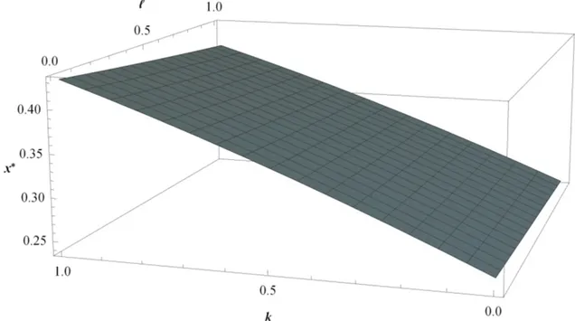
In this section, we examine the results for standard uniformly distributed realized demand, Y ∼ U (0, 1) with F (y) = y, f (y) = 1 and E(Y) = 1/2. Again we assume that supply functions that correspond to prices are linear functions: S(x) = α+βx

and S(Y ) = α + βY where α ≥ 0 and β > 0 on R+_{. Given our assumptions, the}

optimal commitment value x∗ where β(k + l) 6= 0 is found by plugging µ = 1/2, δ = 1 as follows: x∗ = − " α(−k − l) − 2β +p(k + l)2_α2_{+ 2(k + l)(2 + k)αβ + (4 + (1 + k)(k + l))β}2 β(k + l) #

For simplicity, when α = 0, the optimal commitment value the x∗ is reduced to the following expression:

x∗ = p((1 + k)(k + l) + 4) − 2

(k + l) (3.9) According to the optimal commitment value formula in 3.9, Figure 3.1 shows the optimal commitment values that correspond to the each combination of (k, l) within the range of 0 and 1. It represents the change in x∗with respect to penalty parameters k and l. The positive effect of k and negative effect of l on x∗ that we present in Proposition 2 can be seen clearly in this figure. Additionally, it can be seen that when the values of both k and l go to 0 (no penalty parameters in the real-time market), the limit of expression (3.9) is 0.25, meaning that the optimal commitment value is 0.25 (µ₂). However, in this special case one could expect the optimal commitment value to be 0.5 (µ) because of the uniform dis-tribution setting. This outcome supports our assertion in Proposition 5 which is the distribution company has incentive to underbid.

Figure 3.2 represents several k and l combinations that gives the same optimal commitment value. For instance, the (k,l) combinations (0.02,0.2), (0.05,0.8) and (0.06,1) gives the same optimal commitment value, which is 0.25, whereas the (k,l) combinations (0.72,0), (0.8,0.43) and (0.9,1) gives 0.4. When k and l combinations are selected within the range of [0,1] (as it is currently selected in practice), they incentivize the company to commit for some specific values such as such as 0.25, 0.275, 0.3, 0.325, 0.375, 0.4, 0.425 and 0.448 to maximize

Figure 3.1: The change in optimal commitment value with respect to penalty parameters k and l, where Y ∼ U (0, 1).

its profit. In the current practice where k and l are 0.3, a company’s optimal commitment value is found as 0.31 in our setting. The maximum commitment value that could be observed in Figure 3.2 is 0.448. Therefore, the distribution company can commit 0.448 at maximum for all possible combinations of k and l in the current range. However, it should be 0.5 for our special case. This finding indicates that the current range of penalty parameters defined by Energy Market Regulatory Authority still leads distribution company to underbid.

In Figure 3.3, the range of k and l parameters are extended to [-2,2] and the counter plots are provided for the positive optimal commitment amounts. The combinations which incentivize the company to commit expected optimal commitment value, 0.5 are identified as (0.6,-2.2),(1,-1),(1.4,0.2),(2,2). It is seen that for the true forecast value, the penalty parameter l can have both positive and negative values that supports the result that we show in Proposition 4.

The results of Figure 3.2 and 3.3 implies that as long as these penalty param-eters are chosen in the range of [0,1], the distribution company is not forced to forecast or report the true forecast value which is 0.5 for our special case.

0.25 0.275 0.3 0.325 0.375 0.4 0.425 0.448 0.0 0.2 0.4 0.6 0.8 1.0 0.0 0.2 0.4 0.6 0.8 1.0  ℓ

Figure 3.2: k and l combinations for different optimal commitment values where k, l ∈ [0, 1] and Y ∼ U (0, 1)

0

0

0.05

0.05

0.1

0.1

0.2

0.2

0.25

0.25

0.3

0.3

0.4

0.4

0.48

0.48

0.5

0.5

0.6

0.6

0.7

0.7



ℓ

Figure 3.3: k and l combinations for different optimal commitment values where k, l ∈ [−2, 2] and Y ∼ U (0, 1)

Chapter 4

An application: Empirical

calibration with real data

We work with real demand data to examine the effect of penalty parameters based on different demand characteristics such as hour, day, season, region and sectoral demand profiles. In previous anaysis, we took realized demand as uniformly distributed. However, for these anayses, we use real data and find emprical distribution functions for the realized demand in every anaysis. The data that we work on consists of the load profiles of 21 distribution companies that cover the energy needs of 7 regions in Turkey for the months between September 2013 and August 2014 is obtained from the Energy Market Regulatory Authority of Turkey (EMRA) website [41]. The data also includes consumption amounts for different sectoral demand profiles such as household, industrial, commercial, agricultural irrigation and lightening. Once the data to be used are determined, the data are normalized on an hourly basis, so that it becomes compatible with each sectoral demand profile.

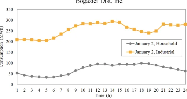
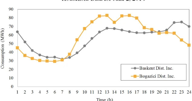
The demand data that we work on shows differences according to hours, sea-sons, regions and sectoral demand profiles. For instance, Figure 4.1, 4.2 and 4.3 show the hourly household and industrial data for a winter month (January) and a summer month (June) for Baskent distribution region and Bogazici distribution

region. As can be seen in Figure 4.1, the consumption amounts differ for winter and summer seasons and the time of the day. For example, in every hour, the consumption amounts in winter day (January 2) are greater than the amounts in summer day (June 2). In addition to that, the maximum consumption amount seen on January 2, 2014 is observed at 9:00 p.m., whereas, it is seen at 11:00 p.m. in June 2, 2014. Moreover, the sectoral demand profile differences can be seen in Figure 4.2. The industrial demand is greater than the household demand in each time period of the day. Figure 4.3 also shows the demand vary according to distribution regions: Baskent and Bogazici.

Hence, as the hourly demand data shows high variety, for our analysis, the realized demand distribution is found by fitting empirical demand distribution functions to the hourly data by Mathematica. Based on the best distribution fits for each analysis, we find the expected profit of the distribution company (can be seen in equation 3.3) by taking S(x) = α + βx and S(Y ) = α + βY where α = 0 and β = 1 for simplicity and obtain the optimal commitment amounts. We also examine how the effects of penalty parameters on the optimal commitment amount vary based on time of the year, seasons, regions and sectoral demand profiles.

In our analysis, we first show that the penalty parameters could be chosen differently for different times of the year such as seasons, days or even the hours. Then, we perform the same analysis on the two different distribution regions in Turkey: Baskent distribution region and Bogazici distribution region. Baskent distribution region includes seven mid-north cities of Turkey including capital Ankara and Bogazici region includes the European side of Istanbul. Results show that effect of the penalty parameters depend on the regions significantly. Finally, we obtain similar results on sectoral demand profiles such as household and industrial.

Figure 4.1: Consumption amounts of the households of Baskent Distribution Inc. for the dates of January 2, 2014 and June 2, 2014 with respect to time.

Figure 4.2: Consumption amounts of the households and industries for Bogazici Distribution Inc. in January 2, 2014 with respect to time.