BUSTLE, a new circuit simulation tool

I ' A - ш ш : с т с ш т . ш м і л т т н t o o l

:

' А ш т ш

втштт-

т о

:;Т

н і

■

ёттжтшт-ш

il s

.

: ■

а ш

: £

lsc

^

q

#İÇS іШ ш вм нт ш

.viï4.· t?» и ’.Г; İ;İV.W «ьч^ >*'·ν· w-Ä' «w v·'·^' ·*· »и*- vJ ' -Ій ííS-S C e 'I ^ C i ííS-S ííS-S ':

0

£ ' Ş ^ t Â İ İ i î ¥ ^ ^ ö r . "Η ·£ ;Й!

2 0

У Ш р ^ Щ

11

"Ш :' V; ’■ : ' · r;£!Ä O r ' ^ ; ;

- М Д І Т Ё Я І C Æ 'i e r E N Ô S ^ · '.:

J:;;.:.,.· ώ/·Μϋ^- . . ♦W '.«.*'4Ä'

BUSTLE, A NEW CIRCUIT SIMULATION TOOL

A THESIS

SUBMITTED TO THE DEPARTMENT OF ELECTRICAL AND ELECTRONICS ENGINEERING

AND THE INSTITUTE OF ENGINEERING AND SCIENCES OF BILKENT UNIVERSITY

IN PARTIAL FULFILLMENT OF THE REQUIREMENTS FOR THE DEGREE OF

MASTER OF SCIENCE /M. L

:-.-By

M. Murat Alaybeyi

July 1990

τ κ .

I certify that I have read this thesis and that in my opinion it is fully adequate, in scope and in quality, as a thesis for the degree of Master of Science.

■ / h U ^

Prof. Dr. Abdullah Atalar(Principal Advisor)

I certify that I have read this thesis and that in my opinion it is fully adequate, in scope and in quality, as a thesis for the degree of Master of Science.

Assoc. Prof. Dr. Mehmet Ali Tan

I certify that I have read this thesis and that in my opinion it is fully adequate, in scope and in quality, as a thesis for the degree of Master o f Science.

.A

"'"Assoc^ ^ rof.' Ayhan Altıntaş

Approved for the Institute of Engineering and Sciences:

/V y ________ Prof. Dr. Mehmet Bafay

ABSTRACT

BUSTLE, A NEW CIRCUIT SIMULATION TOOL

M. Murat Alay beyi

M.S. in Electrical and Electronics Engineering

Supervisor: Prof. Dr. Abdullah Atalar

July 1990

A new circuit simulation tool, BUSTLE, using Asymptotic Waveform Evalua­ tion (AW E) technique and Piece-wise Linear (P W L ) models, is implemented. The results are very promising, especially for large circuits.

This piece of work, in cooperation with [1], explains the techniques used in the simulator BUSTLE, such as

• efficient LU decomposition of the sparse matrices,

• using derivative and integral moments in order to get rid of the instability problem,

• combining the PWL approach with AWE in transient analysis,

and illustrates some simulation results.

ÖZET

BÜSTLE, YENİ BİR DEVRE SİMÜLATÖRÜ

M. Murat Alaybeyi

Elektrik ve Elektronik Mühendisliği Bölümü Yüksek Lisans

Tez Yöneticisi: Prof. Dr. Abdullah Atalar

Temmuz 1990

BÜSTLE, asimptotik eğri tahmini ve parçalı doğrusal yaklaşımını kullanan yeni bir devre çözümleme programıdır. Elde edilen sonuçlar, özellikle büyük devreler için oldukça olumludur.

Bu çalışma, [

1

] ile birlikte, BUSTLE’de kullanılman bazı metodları açıkla­ maktadır. Bunlar arasında

• seyrek elemanlı matrislerin etkili üçgensel ayrıştırılması,

• asimptotik eğri tahmini metodunun kararsızlık problemini çözmek için türev ve entegral momentlerin birlikte eşleştirilmeleri,

• zamanda geçici inceleme için asimptotik eğri tahmini ve parçalı doğrusal yaklaşım tekniklerinin birleştirilmesi

sayılabilir. Son olarak bazı simülasyon sonuçları verilmiştir.

ACKNOWLEDGMENT

My first debt is to Prof. Abdullah Atalar who has taught me the meaning of the word “research” , and provided perfect dosage of criticism and unfailing support throughout the project.

1

am thankful for his proper combination of justice and mercy on deadlines to ensure the completion of this thesis. I explicitly want to acknowledge the support of Assoc. Prof. Mehmet Ali Tan for his critical guidance and useful advice. In addition I am grateful to Prof. Ronald Rohrer of Carnegie Mellon University not only for his encouragement and suggestions but also for initiating the research.

I owe debts of gratitude, too, to Cemal Tamer Dikmen and Satılmış Topçu who are members of CAD group in Bilkent University, for their co-operation in the project. This thesis would not have existed without their contributions. No brief statement can adequately acknowledge the many kinds of help that I have received from Cemal both in the project and in the course of preparing this thesis, even the “acknowledgment” part.

A special note of thanks is due to another contributor. Prof. Erol Sezer for his stimulating insights, and to Assoc. Prof. Ayhan Altıntaş for his com­ plementing study. I am indebted as well to Mujtaba Fidaul Haq for his co­ operation in forming the LU package, and to Gözde Bozdagi, Gökhun Tanyer and Mustafa Karaman for their helps in shaping the project in its early stages. I feel obliged to mention Ogan Ocali and his nice discussion as well as his great pleasure in the exchange of ideas often on the way home from the office at midnight.

Finally I owe a measure of gratitude to my respective institution, Bilkent University and to the sponsor of the project NATO-SFS.

Contents

1 IN T R O D U C T IO N 1

2 DC ANALYSIS 4

2.1

Determination of the Operating P o i n t s ... 4

2.2 Modeling of Nonlinear D e v ice s... 5

2

.

2.1

Modeling of two-terminal nonlinear d e v ice s...

6

2

.

2.2

Modeling of three-terminal nonlinear d e v ic e s ... 7

2.3 The Algorithm U s e d ...

8

3 LU D EC O M P O SITIO N 10 3.1 The Function of LU D e co m p o sitio n ...

11

3.2

Implementation of the Program Taking Various Aspects Under C on sid era tion ...

11

3.2.1 Criteria of E ffic ie n c y ...

11

3.2.2 Possible Data Structures and the Data Structure Actu­ ally Used

12

3.2.3 Methods Generally Used to Increase the Efficiency . . . . 18

3.2.4 Our Strategy for Pivot S election ... 19

3.3 Some of the Tricks Used in the S o f t w a r e ... 20

3.3.1 Memory A llo c a t io n ... 20

CONTENTS vm

3

.

3.2

Listheaders and Multiplication T a b l e ...

22

3.3.3 Representing the Values with Two F ie ld s ...'. 24

3.3.4 Multiple Pivot C a n d id a tes... 24

4 Asymptotic Waveform Evaluation 25 4.1 Using the Combination of Derivative and Integral Moments to Obtain Stable Approxim ations... 26

4.2 Transient Analysis Using AWE 27 5 RESULTS 29 6 H O W TO USE BUSTLE 45

6.1

INPUT FORM AT 45

6.2

CIRCUIT D E S C R IP T IO N ... 46

6.3 BEGIN CARD, COMMENT CARDS, END C A R D ...46

6.3.1 Begin C a r d ... 46

6

.

3.2

Comment C a r d ... 47

6.3.3 End C a r d ... 47

6.4 ELEMENT CARDS 47 6.4.1 R esistors... 47

6.4.2 Capacitors and Indu ctors... 47

6.4.3 Linear Dependent Sources 48 6.4.4 Independent Sources (Time Invariant) 50 6.4.5 Time Varying Independent S o u r c e s ... 50

6.5 PW L D E V IC E S ... 51

6.5.2 Three Terminal PW L D e v ic e s ... 51

6.6

MODEL C A R D S ... 52

6

.

6.1

Two T e r m in a ls ... 52

6

.

6.2

Three Terminals 52 6.7 CONTROL CARDS

54

6.7.1 TR AN C a r d ... 54 6.7.2 PRINT Card 54 6.7.3 PLOT C A R D ... 55 6.7.4 OPTIONS C a r d ... 55

6.8

EXAM PLE INPUT FILE 56

7 Conclusion 59

List of Figures

2.1

(a) Representation of a two-terminal nonlinear device; (b) i-v characteristics of a two-terminal nonlinear device...

6

2.2 Representation of a three-terminal nonlinear device...

8

3.1 A possible one dimensional data structure for the M matrix

12

3.2

A possible two dimensional data structure for the M matrix 13

3.3 Representation of a 4 X 4 sparse matrix having only

6

elements, according to the structure we used... 14

3.4 Structure of (a) a panel, and (b) a node ... 15

3.5 The structure of Listheaders and Multiplication T a b le ... 23

5.1 Pillage’s

6

th order RLC circuit 30

5.2

Output waveforms of the capacitor voltages, for the circuit in Fig. 5.1, computed using different minorder values. 32

5.3 An

200

’th order RLC ladder c i r c u i t ... 34

5.4 Output waveforms of the node voltages 15,

101

and

201

(the volt­ age on the 500 ohm resistor), for the

200

’ th order RLC circuit, computed using BUSTLE with different minorder values, and S P I C E ... 35

5.5 Full-wave rectifier c ir c u it ... 36

5.6 Output waveforms of BUSTLE and SPICE for the full-wave rec­ tifier c i r c u i t ... 36

LIST OF FIGURES XI

5.7 CMOS NOR c ir c u it...

37

5.8 Piece-wise Linear NMOS model used, in the simulation of the CMOS NOR g a t e ...

37

5.9 The output waveform of the CMOS NOR g a t e ... 38

5.10 The operating regions of MOSFETs in the simulation of the CMOS NOR g a t e ...

39

5.11 A Simple Flip-Flop. The input file for this circuit is given at the end of the

6

th chapter... 41

5.12

The plotting routine of BUSTLE showing the Flip-Flop outputs. 42

5.13 The Ring Oscillator Circuit ... 42

5.14 Transient analysis of the ring oscillator c i r c u i t ... 43

5.15 Simulation results of BUSTLE, for CMOS Full-Adder circuit. First two waveforms are the inputs, the other two are SUM and CARRY outputs respectively, (carry-in is grou n ded)... 44

List of Tables

5.1 Approximate Poles for resi^onse at C

2

and the actual poles of

the circuit. 30

5.2

Trials of BUSTLE to find a second order approximation and

conclusion with a third order approximation. 30

5.3 Total execution time list for different minorder requirements . . 31

5.4 Total execution time list of the

200

’th order RLC ladder for dif­ ferent minorder requirements, and the normalized rms difference

from SPICE. 33

5.5 The CPU time for some major functions of BUSTLE, measured in the simulation of the

200

’th order RLC circuit (minorder=3). 33

5.6 Total execution time list of the full-wave rectifier circuit, and the normalized rms differences with lOOOpt SPICE waveform. 34

Chapter 1

INTRODUCTION

Simulation plays an important role in the design of integrated circuits. Using simulation, a designer can determine the functionality and the performance of a design before the expensive and time-consuming step of manufacture. BUSTLE, (Bilkent University Simulation T ool for Linearized Environment), is a circuit level simulator determining the analog waveforms for the branch voltages and currents and the node voltages.

Circuit simulation tools, with different accuracy and speed, are used in cir­ cuit analysis and design. The accuracy and speed requirements vary depending on the type and size of the circuit, and the aims of the user. There is a trade-off between the accuracy and the speed of the simulation. This trade-off assumes the most important role when the number of elements increases prohibitively as is the case in VLSI circuits.

The extensive computations and thus very long simulation time are mainly due to the complex nonlinear characteristic of devices and the large number of iterations for computing the transient response in timing analysis. Most of the circuit simulators employ various numerical and iterative methods (e.g. New­ ton Raphson) to find the operating points of nonlinear circuits and numerical integration methods (Forward Euler, Backward Euler, Trapezoidal, etc.) to compute the transient response of energy storage elements.

Aspects of stability, convergence and hence completion of the job in a suc­ cessful manner are all important issues for circuit simulators. Moreover the models of new devices resulting from the emerging technology must be easily put into a simulator. Otherwise, the simulator may become obsolete in a short time. The simulator should have provisions such that even the user has the capability of doing this integration.

CHAPTER 1. INTRODUCTION

BUSTLE is developed, with the motivation of the above facts. The first aim is to complete the simulation successfully without any problem such as conver­ gence. BUSTLE employs Asymptotic Waveform Evaluation (AWE) technique instead of numerical integration methods, in order to compute the response of energy storage elements.

Piece-wise linear (PW L) representation is used to characterize the nonlinear elements. The main reason to choose the PW L characterization is to avoid solving nonlinear equations and to deal with a set of linear equations to decrease the time complexity and guarantee the convergence in DC Analysis. AWE is mainly for linear(ized) circuits. Thei'efore, the use of PW L approximation makes the utilization of AWE easy and efficient for nonlinear devices.

Another important advantage facilitated by PW L approximation is that the user can define his own device models for nonlinear devices easily. Subse­ quently, it provides a considerable flexibility to the user for choosing his own model and determining the trade-off between speed and accuracy in the simu­ lation. This also renders the simulator independent of the trends of technology.

Consequently, PW L approach brings the advantages of guaranteed DC con­ vergence, efficient usage of AWE, and user defined modeling property.

While using AWE, transient analysis is the part that calls for most of the attention and care. Since the approximate poles and the residues are found for any output of the circuit, only a simple plotting routine does the AC analysis. Note that it is also possible to give an approximate proper rational transfer function of a system in terms of s. The sensitivity analysis using AWE tech­ nique may also be performed with a little additional cost [5] [20].

BUSTLE is the result of a co-operative study of the CAD group in the Department of Electrical and Electronics Engineering of Bilkent University. The whole of the program is written in C, using the UNIX operating system and some programming tools (i.e. Lex, Yacc) and SUN 3/110 Workstations. This thesis is a complementary work with [1]. Some important points are not examined in detail but referred to [

1

].

The following chapter, DC analysis, discusses piece-wise linear modeling, and determination of the operating points using PW L approach. Chapter 3 is about the implementation of LU decomposition of sparse matrices on the computer. This chapter mainly deals with the data structures and algorithms used. Chapter 4 consists of a short description of AWE technique, and the mo­ ment matching algorithm used in the implementation. A detailed examination

CHAPTER 1. INTRODUCTION

of the concepts of this chapter can be found in [

1

]. Then merging PW L with AWE for the transient analysis is discussed in the last section.

Chapter 5 is a collection of some simulation results. Some other examples can be found in [

1

]. This chapter illustrates the advantages that is brought by BUSTLE. The results are compared with those of SPICE. Chapter

6

is a guide for users, and finally the conclusions and the future work can be found in Chapter 7.

Chapter 2

DC ANALYSIS

The solutions to a circuit with DC inputs are called operating points. The term D C analysis refers to the determination of the operating points. The behavior of non-linear circuits are quite different from that of linear circuits. Though there may be no solution or multiple solutions for a non-linear circuit, there is always a unique solution for a linear circuit. BUSTLE uses piece-wise linear (PW L) techniques to determine the operating points of a circuit. Therefore, a nonlinear network is replaced by a piecewise-linear network with a correspond­ ing simplification of the problem. Consequently, solution of nonlinear algebraic systems of equations are reduced to the solution of a set of linear systems of equations :

M x = b (2.1)

where M is the matrix that describes the resistive network, and b is the source vector.

2.1

Determination of the Operating Points

The general methods used to determine the operating points are mesh analysis, nodal analysis, and the tableau analysis. BUSTLE uses tableau analysis which is a completely general analysis method and works for all linear circuits. This method avoids some restrictions caused by nodal and mesh analysis and con­ ceptually it is simpler than the others. Tableau analysis consists of writing out the complete list of linearly independent KCL equations, linearly independent KVL equations, and the branch equations. KCL can be expressed as

CHAPTER 2. DC ANALYSIS

whereas the KVL is given by

V

6

- =

0

(2.3)

where A is the reduced incidence matrix [24], it is the vector containing branch currents, v;, and v „ are the branch and node voltages respectively.

Branch constitutive equations can be written as

G vt + R Í

6

= w (2.4)

where w is the vector including the independent current and voltage sources, as well as the influence of initial conditions on capacitors and inductors. This vector also includes the equivalent sources due to linearization of nonlinear elements. Equations (2.2)-(2.4) can be put into one matrix equation.

I 0 G 0 A R M -A^ 0 0 V

6

'

0

‘ h =

0

. . w (2.5)

Listing the tableau equations, none of the variables is eliminated so all three vectors Vt, ij, and v „ are present as variables. Since we must have as many equations as there are variables, it is clear that the price we pay for the increased generality is that the tableau analysis involves many more equations than node analysis does. In computer-aided circuit analysis, however, this objection turns out to be an advantage because the matrix associated with tableau analysis is extremely sparse which brings the benefits of highly efficient numerical algorithms. The algorithms and the data structure used to solve this sparse systems of linear equations are described in Chapter 3.

2.2

Modeling of Nonlinear Devices

Modeling is the process by which the electrical properties of a non-linear device is represented by means of mathematical equations or tables. Physical device models usually involve many complicated equations. Typical timing studies have shown that the major part of the computational effort in network analysis is spent in evaluating these complicated relationships. Further, most analysis methods also require derivatives of the model equations, which is a cumbersome and error-prone task for the designer. The iterative methods, such as Newton- Raphson, to solve the nonlinear equations do not guarantee the convergence. In

CHAPTER 2. DC ANALYSIS

+

V ..

6

b (a ) (b)

Figure

2

.

1

: (a) Representation of a two-terminal nonlinear device; (b) i-v characteristics of a two-terminal nonlinear device.

order to avoid these problems, piece-wise linear (PW L) representation is used in BUSTLE for the modeling of nonlinear devices. Table models are employed to describe two and three terminal nonlinear devices.

2.2.1

Modeling of two-terminal nonlinear devices

Consider a two terminal element as shown in Fig.

2

.

1

.a. If the voltage v across the element, and the current i which enters the element satisfies /( u , i) =

0

for every time instant, it is called a resistor. Probably the most familiar circuit element is the two terminal linear resistor. Linear resistor is a special Ccise of the resistor and Ohm’s law states that, at all times

/ ( u , i) = v — R i = i — G v = 0

(2.6)

where the constant R is the resistance and the constant G is the conductance. Equation 2.6 can be represented in either the i-v plane or the v-i plane.

The i-v characteristics of two-terminal nonlinear resistors is approximated with a piece-wise linear model, passing through some sample i-v values which are given by the user. BUSTLE assumes that the i-v characteristics is linear between these points, so that the characteristics becomes a combination of linear segments. By using these values, the resistance Ri or the conductance Gi, and the equivalent source to; due to linearization of a two-terminal nonlinear device can be calculated very easily, where I is the segment number. The branch equation of the /th segment of an element can be written as

CHAPTER 2. DC ANALYSIS

i — "f* Giv V = -|- Rit and, in general,

G/ V t + R; it = W ; + w

The tableau equations can be written as follows:

0 A 0 R/ 0 I 0

G;

V t 0 ’ 0 ' h 0 + 0 . - . . w

or in a more compact form

M / X/ = W/ + w

(2.7)

(

2

.

8

)

(2.9)

(2.10)

The subscript / denotes the segment in which the network operates. The right-hand-side vectors denote the equivalent sources due to linearization and the independent sources respectively; they are written separately for clarity.

2.2.2

Modeling of three-terminal nonlinear devices

Three-terminal nonlinear devices are represented as a combination of two 2- terminal devices placed between the three nodes as shown in Figure

2

.

2

. The parasitic capacitors are also included in the device model. The values of these capacitors are given in the model card.

The characteristics of a three-terminal nonlinear device is defined by two branch equations and a number of boundaries for each region. These two branch equations define a 2-dimensional hyperplane in the 4-dimensional space which describes the characteristics of the nonlinear device where the bound­ aries describe the region at which these equations are valid. The two branch equations for the three-terminal nonlinear devices are of the general form:

OiUi + 02^2 + «3*1 + «4*2 +

«5

= 0 (2.11)

and at most three of the coefficients a i,a

2

, «

3,«4

can be nonzero. This does not impose any restriction on the generality since one of them can be elim­ inated using the other plane equation. The boundaries are described by the inequalities of the following form.

CHAPTER 2. DC ANALYSIS

©

+

V,

Figure

2

.

2

: Representation of a three-terminal nonlinear device.

and at most two of the coefficients

01

,

02

,

03,04

can be nonzero since two of the variables can be eliminated, using the two branch equations of the region. Each nonlinear device must contain a segment that satisfies the origin (both the equations and the boundaries) in order to have a valid solution when all of the independent sources are killed. This is required in order to start the DC analysis which will be described in the next section. Also this rule does not impose any restriction on the generality, since any device which does not fit this rule can be modeled with a PW L device satisfying this rule and an independent current source in parallel.

2.3

The Algorithm Used

For DC solution, all inductors and capacitors are replaced by independent sources. Given a valid solution Xq for an arbitrary source vector yo, satisfying

the boundaries of the region Rq,

M o Xo = Wo -I- yo (2.13)

we would like to find the solution x and the region R j for a given source vector

y

M / X = w / -f- y. (2.14)

The algorithm used for the DC Analysis has been derived from the Katzenel- son’s algorithm [9 ,

10

] which guarantees the convergence in the DC Analysis [

8

].

CHAPTER 2. DC ANALYSIS

The modified version of the Katzenelson’s algorithm, used to find the solution X and the final operating region set R f, is as follows:

1

. Set i = 0.

2. Solve X from M i X = Wi + y.

3. If X satisfies the boundaries of Ri then TERMINATE, else GOTO 4.

4. Let A be the ratio of the distance from Xi to the first region boundary crossed when traversing from Xj to x, to the distance from Xi to x.

5. Compute Xi+i as

Xi+i = Xi + A(x - Xi).

6

. Set Ri+i to the neighbor region of Ri separated from it with the first crossed boundary.

7. Increment i and GOTO

2

.

Note that for the first DC analysis, Xo and yo can be selected as

0

, since by definition, every nonlinear element is modeled to have a passive resistive segment satisfying the origin, and

0

is the solution when all the independent sources are killed. It is obviously a poor starting point, but that is the only valid solution known initially. Afterwards the lastly found operating points are chosen as Xq, yo, and Rq. We are expected to do less computation starting

from the last solution, since it is more probable that the old solution is closer to the new one than the origin (

0

).

Chapter 3

LU DECOMPOSITION

The major part of the computation time of the circuit simulation tools is spent on finding the solutions of sets of linear equations. BUSTLE uses LU decompo­ sition and Forward and Backward Substitutions to solve these equations. This section is a detailed explanation of the methods used by BUSTLE to solve linear sets of equations efficiently.

The simulator uses piecewise linear (PW L) approach in DC analysis which is performed several times throughout the program. In DC analysis Sparse Tableau Analysis is used which in the end , boils down to finding the solution of the matrix equation M x = b. The matrix M is usually a very sparse matrix for large circuits, having only

0

.

1

% or fewer non-zero elements on the average. DC analysis generally performs a set of LU decompositions in order to find the operating segments of the PW L devices. Most of the LU decompositions performed by the simulator are this type. There is also another LU decompo­ sition following each DC analysis in order to find the steady state solutions of the circuit.

Solving a set of linear equations on the computer efficiently is a problem which has been investigated for a long time and is also being investigated now [14, 13,

11

]. The problem gets even more complicated when the set of equations form a sparse matrix. The problem springs from the fact that it is not straightforward to harvest the advantages of the sparsity of the matrix that can be translated to profitable gains in memory consumption, computational speed and accuracy.

CHAPTER 3. LU DECOMPOSITION 11

3.1

The Function of LU Decomposition

This part of the progrcim is a package of C functions used to quickly and accurately solve large sparse and real systems of linear equations which can be expressed as M x = b. The package is optimized for speed using a good strategy of pivot selection and is able to perform numerical pivoting to avoid numerical inaccuracy in the solution. What it actually does is,

• It decomposes M into two triangular matrices such that M = LU , where L is a lower triangular matrix and U is an upper triangular matrix.

• then it solves the y vector from L y = b by forward substitution which is a very easy task. Next U x = y is solved by a backward substitution where y is found from the forward substitution. This whole process is called Forward and Backward Substitution (FBS). Once the LU decomposition is performed, the x vector can be solved for the same M matrix and different b vectors using only FBS.

3.2

Implementation of the Program Taking Various

Aspects Under Consideration

3.2.1

Criteria of Efficiency

Efficiency of the program is characterized by the following points

C o m p u ta tio n tim e : Since the speed of the whole simulator crucially de­ pends on the computation time of both the LU factorization and FBS (especially for large circuits), they must be executed as fast as possible. Minimization of the computation time is one of the major concerns for us while developing the program. We have been extremely cautious to cut off any redundancy in the computation to make the program as fast as possible.

A c c u r a c y : Since various routines of the simulator uses the LU factorization and FBS quite frequently, the error in computing them has an immense effect on the overall accuracy of the simulator. It should be mentioned here that algorithms used to compute LU decomposition and FBS in­ variably causes an error which is cumulative in nature, though the error

CHAPTER 3. LU DECOMPOSITION 12

Row Panel

Figure 3.1: A possible one dimensional data structure for the M matrix

incurred by the simulator itself may or may not be cumulative. Various methods like numerical pivoting, minimization of fill-in’s etc. which will be described later, are used in order to make as little compromise with the accuracy of the program as possible. If necessary, the program has the capability of doing iterative refinements on the solution.

In order to increase the accuracy one has to make frequency scaling [4], which is not related with LU decomposition.

M e m o r y C o n s u m p tio n : It is quite reasonable to expect that owing to the sparse nature of the matrix M , an efficient and compact use of the mem­ ory is possible. But minimizing the consumption of the memory may not optimize the overall performance of the program. In this program though we have been careful not to make waste of memory allocation, we did not seek optimizing the program from the memory consumption standpoint.

3.2.2

Possible Data Structures and the Data Structure

Actually Used

There can be several ways to store the sparse matrix in an efficient form. Two of the feasible data structures are illustrated in Fig. 3.1 and Fig.

3

.

2

, while the data structure we have actually used is shown in Fig. 3.3.

CHAPTER 3. LU DECOMPOSITION ₁₃ Rüvv Panel

Column Panel

Other ' fie ld s other f ie ld s A A y\ I A A A A_{N. A} 1 A

A

A

A A

y\.

A A j\

CHAPTERS. LU DEC0A4P0SITI0N 14 COLUMN PANEL ROW PANEL N2 CO Q.' ÜJ X I-o NZ CO LL· LÜ X H r-i OR N0 OR NO L. JZ NODE

7

Figure 3.3: Representation of a 4 x 4 sparse matrix having only

6

elements, according to the structure we used.

arrays of structures. Each element of row or column panel has five fields. They are shown in detail in Fig. 3.4, and their function is described below.

o r : It is the original row or column number which remains unchanged through­ out the program.

n o : It indicates the order of selection of a row or column as the pivot row or column.

b e g in : This is a pointer field pointing to the first element of the row or column.

m a x : This pointer field points to the largest element in magnitude of the row or column.

N Z : The number of nonzero elements in a row is known as NZUR and the NZ field of a row stores the NZUR of that row. Whereas, the number of nonzero elements in a column is known as NZLC and the NZ field of a column panel stores it.

CHAPTER 3. LU DECOMPOSITION ₁₅

( b )

CHAPTER 3. LU DECOMPOSITION 16

On the other hand, the nonzero elements of the matrix are stored in “nodes” which are connected both to the panels and to each other. The fields of a node are illustrated in Fig.

3

.

4

.b and are described below.

row p an el p o in te r : This is a pointer field pointing to the specific row in the row panel which it belongs.

co lu m n p an el p o in te r : This is a pointer field pointing to the specific col­ umn in the column panel which it belongs.

righ t : This pointer points to the node on the right, if there is any.

d o w n ; This pointer points to the node below, if there is any.

val, value : They contain the value of the nonzero elements and they are described in section 3.3.3 in more detail.

n e x tm a x m a x , p re v io u s m a x m a x : These fields are used to link the pivot candidates to each other, and also to mark the elements which are not pivot candidates.

In order to solve a matrix equation using LU decomposition we must per­ form the following operations n times where n is the order of the M matrix.

1. Pivot selection

2. Row and column interchange

3. Normalizing the pivot row and zeroing the elements under pivot

4. Updatings

And then FBS is performed as many times as required by the simulator.

We are going to calculate the time complexity of the above items for all of the structures mentioned above, then show that the structure we have used performs best.

1

. P iv o t S e le c tio n : The complexity of the calculations made for pivot selection highly depends on the pivot selection algorithm. But it is easily seen that the data structure we have used eases the work of pivot selection for any algorithm.

CHAPTER 3. LU DECOMPOSITION 17

2

. R o w and C o lu m n In terch a n ge : As soon as a pivot is selected we have to interchange the pivot row and column with the ¿’th row and column, where i is the order the pivot is selected. In the data structure we have used, a row or column interchange has time complexity of

0

(

1

) as there is no physical row or column interchange in this structure. Whenever an element is chosen as the pivot, the no field of the row panel of that element is numbered in the order it is selected. For example, if an element say, of the fourth row, is chosen as the pivot at the beginning; instead of interchanging the first and the fourth row, the number field of the fourth row-panel is set to “

1

” . The column interchange is also performed in a similar way. In fact this numbering operation is used for marking a row or column when it is selected, so that in the later operations they are skipped and they are not subjected to any further execution. Although we do not perform any physical interchange, the algorithm behaves as if the interchanges are done physically.

But this is not the case with the data structures in Fig. 3.1 and Fig. 3.2. The first structure has 0 (1 ) time complexity for row interchange, whereas the time complexity of column interchange is O(nfc), where k is the aver­ age number of nonzero elements in a row or column, and n is the order of the matrix. Although k is usually a small number, the performance gets worse as n increases. For the second structure it can be easily shown that the time complexity of both the row and column interchange is 0{kS).

3. N o rm a liz in g th e p iv o t row and z e ro in g th e elem en ts u n d er th e p iv o t : In fact the factorization can be done without the other items but this item is the fundamental job during the LU decomposition. There are two major things to consider in this part. They are

F lo a tin g p o in t o p e ra tio n s (flo p s ): Operations like normalizing the pivot row and multiplications and subtractions in the subsequent rows involve flops which can not be avoided. The computation time to perform floating point operations are the same for all the struc­ tures, as long as the same algorithm is employed in the pivot selec­ tion. It can be shown that the time complexity is 0{nk'^). These operations are generally more time consuming than the non-floating point operations which are mentioned below.

N o n -flo a tin g p o in t o p e ra tio n s : Operations like visiting a node and checking if it is marked or not are non-floating point operations. These operations must be performed in addition to flops to LU fac­ torize the matrix and they vary from structure to structure.

CHAPTER 3. LU DECOMPOSITION 18

4. U p d a tin g s : Tn oi-dc.r to make a proper selection of pivots we have to store certain information about the matrix such as NZU R’s of the rows. This information may change at any step of the LU factorization and hence must be updated whenever undergoes a change. The.se updatings are highly dependent on the data structure, and the algorithm employed. For the data structure we have employed, the updating procedures will be explained later.

3.2.3

Methods Generally Used to Increase the Effi­

ciency

The methods generally used to achieve efficiency are as follows:

Numerical Pivoting

The element by which a row is normalized is known as the pivot element. The selection of the pivot regarding the numerical values of the elements in the matrix is called numerical pivoting. In order not to lose much from accuracy, several type of pivoting strategies can be employed. The most widely used of these strategies are partial pivoting and complete pivoting which are well known pivoting strategies and can be found in any elementary book on numerical analysis [

12

,

11

]. Hence, they are not discussed here.

M in im iz a tio n o f N u m b e r o f Fill-ins

Let’s suppose an is chosen as the pivot, and the pivot row is normalized. While zeroing the pivot column, aji is multiplied with a,·*, and subtracted from ajk, when j > i and ^ > L If ajk was 0 previously, it was not stored in the memory. But now a new non-zero value has occurred at ajk] this is called a fill-in. A fill-in causes the following problems.

1

. A new memory location to be allocated for it which is not very desirable.

2

. An increase in the time complexity, due to a few extra non-flops.

CHAPTER 3. LU DECOMPOSITION 19

4. New fill-ins , which is the most important of the problems, as these new fill-ins, in turn, cause the trouble mentioned in above items and a host of new fill-ins.

So it is clear from the problems mentioned above that we should try to minimize the number of fill-ins. An estimate on the number of possible fill-ins a pivot can cause is { N Z U R — l) X ( N Z L C —1) of pivot row and pivot column, as this is the total number of multiplications that should be performed. These products are then subtracted from ajk, which because of the sparsity of the matrix has a great probability of being zero.

Hence, { N Z U R — 1) x { N Z L C — 1) is a proper estimate on the possible number of fill-in’s a pivot will create. So, the smaller the product, the lesser the number of fill-ins. As can be seen, if either NZUR or NZLC is 1, there is no fill-in. More over the elements in the pivot row(column) are not included in the calculations anymore, which causes a decrease in NZUR(NZLC). All these are very desirable. So it is a good strategy to select the pivot from a row or column whose NZ field is 1, even though the element is not large in magnitude.

3.2.4

Our Strategy for Pivot Selection

Our pivot selecting strategy is a combination of classical numerical pivoting strategies and minimum fill-in strategy. The algorithm used for LU decompo­ sition is described below.

1. A pivot must be the maximum element of both its row and column, in our jargon, we say a pivot must be тахтах (this strict rule is modified in multimaxmax strategy which will be described later). Note that there is at least one maxmax element : the maximum element in the matrix. So there is always at least one pivot candidate which is necessary for the continuation of the job.

2. The elements satisfying the above condition are found, and then among these pivot candidates the one which has a minimum value of the product { N Z U R — 1) X { N Z L C — 1) is selected to be the pivot.

3. Floating point operations are performed according to the selected pivot above. Then we discard the elements in the pivot row and column from the further calculations.

CHAPTER 3. LU DECOMPOSITION 20

4. Because of the operations and discardings there will be changes among the pivot candidates selected according to the first rule. Therefore we must handle these changes by updating maxmax’es.

5. Because of the discardings in “3” , there will be changes in NZUR and N ZLC’s of some rows and columns. We have to register these changes and update the list which is composed of maxmax elements sorted in the ascending order of the products ( N Z U R — 1) x ( N Z L C — 1).

3.3

Some of the Tricks Used in the Software

3.3.1

M em ory Allocation

The package uses dynamic memory allocation, because of the large variety of the input matrices in dimension and spai'sity. The memory allocation per­ formed by the system may be very slow if it is not used judiciously. For example, for a specific type of data structure of size m, allocating memory space to n variables of this structure type separately, that is using malloc(m) n times, is much slower than allocating them altogether by malloc(n * m). For our M matrix, we know the number of nonzero elements from the very begin­ ning. Hence, we can utilize this situation by allocating all the required memory space right at the beginning. In this subsection we will mention some of the procedures which use tricks like this in the memory allocation.

D u p lic a te : At the beginning of the program, the M matrix is set up in the memory. Since we will have to deal with the matrix for a lot of times, we duplicate the matrix to a different memory location and perform the LU factorization on this copy of the matrix. In the very beginning of the program chunks of memory of ec^ual size are allocated for both the original and the copy of the matrix. However the actual size of memory allocated to each of them is a bit larger than the number of nonzero elements in the matrix, which we call the “tolerance” . The tolerance is introduced to take care of the changes in the stencils of the original matrix which may cause an increase in the number of nonzero elements in the matrix, requiring extra memory space.

After the initial set up of the original matrix, memory spaces are allo­ cated for copies of the list-header and panels in a similar way. The only remaining task to be done at this stage of duplication is to copy the web

CHAPTER 3. LU DECOMPOSITION 21

of pointers of the original setup to the duplicate copy. The original setup is full of pointers as was shown if Fig. 3.3, Fig. 3.4 and Fig. 3.5. So if not done cleverly, it can take a long time to duplicate the pointers to their re­ spective position in the duplicate copy. The strategy we have used to copy the pointers which are in fact addresses of memory locations, resembles the method of relative addressing. First of all, the offset, M ->beginning- of-nodes — M copy->beginning-of-nodes, is calculated. Then, this offset is added to the memory address written in the pointer field of the nodes of the original setup and copied to the respective pointer fields of the duplicate. This works if all nodes of the original setup and the duplicate setup are allocated in the same page and hence has a constant relative address difference between them. The same relative copying method is used to copy the panel pointers.

s ta llo c (allocation for stencils) : In order to use the advantage of the infor­ mation that all of the nodes use same amount of memory, the memory allocation is handled by the program. If a memory space for a new node is requested, then since we know how much memory is necessary, there is no need to call a system function. Instead the package routines uses stalloc or falloc.

A few elements of the M matrix can change values or even disappear and a few new elements can appear whenever the stencils of the matrix is changed at the beginning of each LU factorization in a particular sim­ ulation. The function stfree pushes the address of the freed nodes into a stack and the function stalloc allocates memory space for a new element by popping an empty node address from the stack. The tolerance nodes which are allocated at the very beginning of the of the setup are also pushed into the stack.

If, in case, the stack happens to be empty, i.e. there is no free space left, we allocate a new space of memoiy which has STACKPAGE number of more space than previous one and duplicate all the elements ( N Z U R — 1) X [ N Z L C — 1) to the new one. Now, we have STACKPAGE amount of new free space.

fa llo c (fill-in allocation) : During LU factorization of M copy, we will need new space for fill-in nodes, falloc is used in order to provide these new nodes. When the first fill-in occurs, a page of size FILL-IN-PAGE is created, using the system’s allocation command. The pointer indicating the beginning of the page is then pushed into a stack. The page is then used to store subsequent fill-ins until if is full whence a new page is

CHAPTERS. LU DECOMPOSITION 22

created and the pointer showing its beginning address is pushed into the stack.

When a stencil or stencils of M copy is altered by some other routine of the simulator, the M copy is LU factorized from the beginning. Hence the data in the “FILL-IN-PAGE” s become unnecessary and are virtually freed by the procedure ffrce. What actually happens is instead of being freed physically, they are overwritten as new fill-ins occur. This technique serves our purpose better as nearly the same number of fill-ins occur for the handful of stencil changes. This procedure saves us the time of freeing memory spaces and reallocating them.

3.3.2

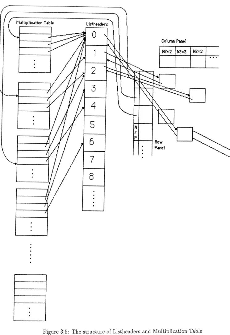
Listheaders and Multiplication Table

In order to implement the efficiency increasing strategies explained in sec­ tion 3.2.4, a separate data structure is constructed. Fig. 3.5, in addition to the structure which stores the nonzero elements of the matrix. A part of this struc­ ture is listheaders which in fact, is an array of nodes whose nextmaxmax fields point to possible pivot candidates (maxmax’es) in an ordered manner. The first element of the array points to maxmax’es whose { N Z U R —l) x { N Z L C — 1) = 0, the second element points to maxmax’es whose { N Z U R —l) x { N Z L C —l) = 1 and so on.

The listheader array facilitates the task of selecting a pivot quite elegantly. We always select the pivot such that it is the maxmax pointed by the non- NULL nextmaxmax pointer of the topmost element of the listheader array. It should be mentioned that with a high probability the nextmaxmax pointers of the upper listheaders will point at some maxmax’es after the updatings have been performed at each operation. Using the data structure, Addmaxmax, which inserts a maxmax to the list pointed by the proper listheader, is a very fast and simple function.

The two way linked list structure if the maxmax elements provides simplic­ ity at the updatings. For example a deletemaxmax operation consists of only two pointer changes. The nextmaxmax fields of the non-maxmax elements are equated to a specific address, called ABYSS, so that maxmax elements can be easily identified.

CHAPTER 3. LU DECOMPOSITION 23

CHAPTER 3. LU DECOMPOSITION 24

3.3.3

Representing the Values with Two Fields

In the sparse tableau analysis, we know that most of the nonzero elements ai'e I ’s or - I ’s. There is no need for a floating point multiplication with these elements, the result is obvious, the number which is multiplied with these elements either stay the same or change sign. In order to speed up using this property we use two fields to store a value. If the value is 1 or -1 we store it in the integer field, val. Otherwise we put a zero into the val field and the number is stored in the double (floating point) field, value.

3.3.4

Multiple Pivot Candidates

We introduce multiple pivot candidates strategy in order to reduce the bad effects of the strict rule, “a pivot must be a maxmax” . Because of this strict rule we may be burdened with a lot of unnecessary fill-ins. For example, an element of numeric value 10, may be selected as a pivot candidate although an element of numeric value 9.5 at the same row has a lower ( N Z U R — 1) x ( N Z L C — 1). In order to prevent such situations, we can allow more than one element in a row or column, to be pivot candidates, which we call multimaxmax strategy. We can normalize every row and afterwards every column, with the maximum element of that row/column, then defining a threshold, select the elements greater then this threshold as pivot candidates. Another way to do this is to define a fast function, may be a function of the power bits of the floating point number, which is a rough measure of the magnitude and then assume all of the elements which has the maximum rough magnitude to be pivot candidates.

Chapter 4

Asymptotic Waveform Evaluation

Asymptotic Waveform Evaluation (AWE) is a recently proposed technique for the approximate pole zero representation of linear time invariant circuits [2] [3]. It is, in fact, a form of Fade approximation [16]. AWE uses the differential state equations

x = A x + Bu (4.1)

to find an approximation for the state variables. We know that, the homoge­ neous solution of 4.1 is of the form

x ,(i) = (4.2)

1=1

where q is the order of the circuit. ki and pi are the residues and poles respec­ tively.

AWE finds an approximation to 4.2 such that

x,(i) =

/=1

(4.3)

where q' is the order of approximation which is smaller than q (in most cases q' <C g), and k\ and p\ are the dominant approximate residues and poles re­ spectively. They are calculated from the moments of the circuit. An important restriction with AWE is that it may produce unstable poles even though the circuit is stable, which is also a major problem for Fade approximation [16] [15]. This problem is overcome by combining differential and integral moments.

The computation of derivative and integral moments, and the calculation of poles and residues using the combination of derivative and integral moments is described in [1].

CHAPTER 4. ASYMPTOTIC WAVEFORM EVALUATION 26

4.1

Using the Combination of Derivative and Integral

Moments to Obtain Stable Approximations

Using AWE, we may find unstable approximations for stable circuits. This is because we are trying to api^roximate a higher order system with a lower order- one. And the moments may give inconsistent information for that lower order system. For example, assume that the original waveform has a negative initial condition and goes to zero at steady state after a large positive overshoot (i.e., the area under the original respoirse is positive). If we use the integral moment for matching, the first order approximation can not find a stable solution. But if we use the first derivative momeirt approximation or a second order approximation (derivative or integral or a combination of both), we can find a stable approximation. We can also conclude with right half-plane (RHP) poles using only derivative moments. So it is a good idea to use an appropriate combination of integral and derivative moments for the calculation of poles and residues of every state variable independently. Here is the algorithm used for this purpose.

• Necessary moments are computed according to the order of approxima­ tion.

• For every state variable DO

(i) Compute the poles using the proper moments (initially start from all integral moments if the user does not redefine this parameter). (ii) If there is any right-hand-plane pole then

If there are no integral moments used then increase the order of approximation by 1, else

replace the highest order integral moment with the next derivative moment, and go to (i) to compute the poles. (iii) Compute the residues.

So, the number of derivative moments used in the approximation is in­ creased one by one until a stable approximation is found or all of the integral moments are replaced with the derivative ones. If a stable approximation can not be found then the order of approximation is increased by one. And we are trying to avoid large orders, due to numerical inaccuracy and increased num­ ber of operations which requires long time for the approximation. But we have

CHAPTER 4. ASYMPTOTIC WAVEFORM EVALUATION 27

observed for a large number of examples that a stable and good approximation can be found before the 5’ th order. If a stable approximation can not be found up to a certain order, (which never occurred for all the examples we tried) the order of approximation is not increased anymore, but the first derivative is used to approximate the response (Forward Euler) to shift in time. After that a new AWE is made with different initial conditions. Note that the dominant approximate poles and residues depend on the initial conditions. Note that, using this algorithm, the order of approximation and the number of derivative moments used in the approximation may not be the same for different state variables. And it is not necessary to approximate all of the states with the same order for transient analysis as far as you find a good approximation for that state variable.

4.2

Transient Analysis Using A W E

In the beginning of the transient analysis, a dc analysis is performed in order to find the operating points. For this dc analysis the capacitors with user defined initial values are replaced with voltage sources of the same value, while the other capacitors are assumed to be open circuits. Similar things are performed for the inductors. Another dc analysis follows in order to find the steady state values. Then we can approximate the state variables with asymptotic waveform evaluation technique, using the initial conditions, steady state values and the linearized circuit itself.

Using AWE wc obtain approxinmte analytic expressions for Ccipcicitor volt­ ages and inductor currents. These expressions are valid on the time axis as long as PW L elements satisfy the boundaries of the set of current operating regions, Ri. In order to find voltages and currents of each device, these expressions are evaluated at certain time instants and using these values as sources, the circuit is solved by a mere substitution (FBS). As we progress over time with steps the nonlinear devices in the circuit may change their segments. If this occurs, we must know the time when one piece-wise linear device, at least, changes its segment. As soon as we realize a segment change, we go back over time and search for the time of segment change. The capacitor voltages and inductor currents at the time instant of segment change, are the initial conditions for the next AWE. The same thing happens when there is an input change at time to- We evaluate the approximate expressions found for energy storage elements and solve the circuit at time Iq by a mere substitution. A new DC analysis is done at time Iq using the new .source vector, and a new AWE is performed

CHAPTER 4. ASYMPTOTIC WAVEFORM EVALUATION 28

for t > Iq . For DC analysis, v/e can use the previous solution and segments (instead of 0 vector) as initial valid solution. This saves a lot of computation.

The selection of the time step in transient analysis is a quite critical issue for the time efficiency standpoint. If the time step is chosen too small, then too many unnecessary computations must be performed. This may even cause the simulation not to terminate in a reasonable time. Conversely too large time steps may cause hirge errors if there exist high frequency poles with large residues. Another drawback of the large time step is that we may skip an over­ shoot of the waveform which may possibly cause a segment change. Therefore, the time step used in transient analysis is dynamically calculated after each FBS. In this calculation, we consider prinicirily the rate of change of the most rapidly changing exponential. There are some parameters used in the calcula­ tion of the tiine step. For example the calculated time step is divided by the SAFETY factor which can be set in the .OPTIONS card. TSLOOPLIM IT is another parameter which is useful if the internal time step turns out to be too small. In a PW L circuit if there is no segment change over a TSLOOPLIMIT time step period, then the time step is multiplied with TSMULT at every time step until a segment change occurs. This causes an exponential increase of the internal time step and prevents an infinite loop due to an error in the calcu­ lation of the time step. BUSTLE has some other parameters for the transient a.nalysis which will not be mentioned.

As a result of dynamic selection of the time step, the simulator spends more effort when there are rapid voltage or current changes, and skips quickly in the time axis if there are slow changes. This provides an event driven feature to the simulator.

Chapter 5

RESULTS

In this chapter, some simulation results of BUSTLE will be presented. Some other results can be found in [1]. The results and computation times of BUS­ TLE is compared with those of SPICE 2G.6. All of the measurements are made at SUN 3/110 workstations. As it is mentioned before, BUSTLE leaves the ac­ curacy speed trade-off to the user by giving him /her a number of options. The minimum order of approximation, the mmorder, which can be given a value in the .OPTIONS card, determines the number of moments matched in AWE. This parameter is an important parameter for the accuracy of the approxima­ tion. For example, it can be selected as 1 for a digital CMOS circuit, but this would not be sufficient for an RLC circuit which has an oscillatory response. The minimum order and also the number of derivatives that will be matched initially can be determined by the user. There are also some other parameters that can be set by the user to improve the accuracy or the speed. Another important feature is that, user can define his own models (or use one from the library) for nonlinear devices. This provides a capability to keep pace with the emerging technology, also user can control the accuracy speed trade-off by choosing the number of segments used for modeling.

E X A M P L E S

1)

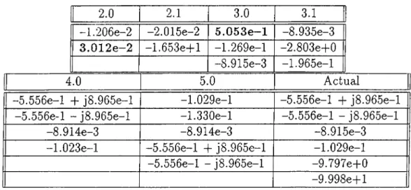
The first example circuit. Fig. 5.1, which is taken from [3], demonstra.tes the usage of derivative and integral moments together, to get stable approxi­ mations. Using basic AWE method [2], we end up with RHP poles for C2 and L3 for a second order approximation, which is not mentioned in [3].

However, using the method described in section 4.1, we can find stable ap­ proximations for all of the state variables. As it can be seen from the Table 5.1, after using the first derivative moment, a stable approximation can be found for

CHAPTER 5. RESULTS 30

1 »-1 IH t2 10 L2 IH Its LS IH

U(t)

_©

Cl _IF C2

IF cs. _IF

r'igure 5.1: Pilla.ge’s 6l.h order RLC circuit

2.0 2.1 3.0 3.1

-1.206e-2 -2.015e-2 5 .0 5 3 e -l -8.935e-3 3 .0 1 2 e -2 -1 .6 5 3e+ l -1.269e-l —2.803e-l“0

-8.915e-3 -1.965e-l

4.0 5.0 Actual

-5 .5 5 6e-l + j8.965e-l -1.029e-l -5.5 5 6e-l + j8.965e-l -5.556e-l - j8.965e-l -1.330e-l -5 .5 5 6e-l - j8.965e-l

-8.914e-3 -8.914e-3 -8.915e-3

-1 .0 2 3e-l -5 .5 5 6e-l -b j8.965e-l -1.029e-l -5.5 5 6e-l - j8.965e-l -9.797e-f0

-9.998e+ l

Table 5.1: Approximate Poles for response at C2 and the actual poles of the circuit.

2.0 2.1 2.2 2.3 3.0

-1.022e-2 -4.301e-9 O.OOOe+0 O.OOOe+0 -8.914e-3 4 .0 3 3 e -2 4 .3 0 1 e -9 -5.404e-fl7 -l.OOle-1 -7.975e-l -1.047e-l

Table 5.2: Trials of BUSTLE to find a second order approximation and con­ clusion with a third order approximation.

CHAPTER 5. RESULTS ₃₁ minimum order

1

compulation time 1.52 sec. 1.72 sec. 1.80 sec. 2.00 sec. 3.13 sec.

Table 5.3: Total execution time list for different minorder requirements

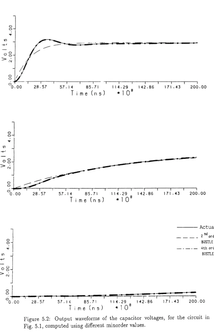
C2, whereas for L3, we can not get rid of RHP poles using a second order ap­ proximation even all possible combinations of derivative and integral moments are tried. In this case the order of approximation is increased automatically, and a stable approximation in the 3’rd order (Table 5.2) is found. But the remaining states are approximated with second order which is the minimum required order. Note that a better approximation for L3 is performed which satisfies the accuracy requirements of the user.

The step responses of 3 different nodes of the circuit in Fig. 5.1, computed for different minorder requirements, can be seen in Fig. 5.2. The execution time list is given in Table 5.3. The computation time of BUSTLE is pretty good. Additionally, for this circuit, BUSTLE finds the results analytically in about 30% of the total execution times listed in the table, and 70% of the execution time passes during the evaluation of the exponentials at certain time instants and simple substitutions.

2)

This example is a 200’th order RLC ladder circuit (Fig. 5.3). Since the circuit is too large, the whole of it is not drawn. But the circuit is a repetition of the ladder. All of the capacitors are 10/if and all of the inductors are lOOmh. The initial voltages of all of the capacitors are given as 0, and the initial inductor currents increments by 1 ma after every 5 inductor, so that the initial currents of the first 5 inductors are 0 ma, the second 5 are 1 ma, and the last 5 are 19 rna. The voltage waveforms of the nodes 15, 101 and 201, are drawn in Fig. 5.4, for different minorder values. The timings and the normalized rms differences ^ from SPICE are listed in Table 5.4.

3)

The third example, Fig. 5.5, is a full wave rectifier. The diodes are

Normalized rms dif ference =

CHAPTER o. RESULTS 32 {n O /i -O o (0 o § . o o 0.00 2 8 . 5 7 5 7 . 1 4 85. 71 T ¡ me ( n s ) Actual 2 order BUSTLE ---^th order BUSTLE \ 114.29

. 1 o'

--

1

----r 142.86 171.43 2 0 0 . 0 0

Figure 5.2: Output waveforms of the capacitor voltages, for the circuit in Fig. 5.1, computed using different minorder values.