ALGORITHMS FOR THE SURVIVABLE
TELECOMMUNICATIONS NETWORK
DESIGN PROBLEM UNDER DEDICATED
PROTECTION
a thesis
submitted to the department of industrial engineering
and the institute of engineering and science
of bilkent university
in partial fulfillment of the requirements
for the degree of
master of science
By
Pelin Damcı
I certify that I have read this thesis and that in my opinion it is fully adequate, in scope and in quality, as a thesis for the degree of Master of Science.
Assoc. Prof. Dr. Oya Ekin Karas.an (Supervisor)
I certify that I have read this thesis and that in my opinion it is fully adequate, in scope and in quality, as a thesis for the degree of Master of Science.
Assoc. Prof. Dr. Hande Yaman
I certify that I have read this thesis and that in my opinion it is fully adequate, in scope and in quality, as a thesis for the degree of Master of Science.
Asst. Prof. Dr. ˙Ibrahim K¨orpeo˘glu
Approved for the Institute of Engineering and Science:
Prof. Dr. Levent Onural Director of the Institute
ABSTRACT
ALGORITHMS FOR THE SURVIVABLE
TELECOMMUNICATIONS NETWORK DESIGN
PROBLEM UNDER DEDICATED PROTECTION
Pelin Damcı
M.S. in Industrial Engineering
Supervisor: Assoc. Prof. Dr. Oya Ekin Karas.an July, 2010
This thesis presents algorithms to solve a survivable network design problem aris-ing in telecommunications networks. As a design problem, we seek to find 2-edge disjoint paths between every potential origin destination pair such that the fixed costs of installing edges and the routing costs are jointly minimized. Despite the fact that the survivable network design literature is vast, the particular problem at hand incorporating fixed and variable edge costs as well as different cost struc-tures on the two paths has not been studied. Initially, an IP model addressing the proposed problem is developed. In order to solve problems of higher dimensions, different heuristic algorithms are designed and results of a computational study on a large bed of problem instances are reported.
Keywords: Survivable network design, Primary and secondary paths, Dedicated protection.
¨
OZET
ADANMIS
¸ KORUMALI G ¨
UVEN˙IL˙IR HABERLES
¸ME
A ˘
GLARI ˙IC
¸ ˙IN ALGOR˙ITMALAR
Pelin Damcı
End¨ustri M¨uhendisli˘gi, Y¨uksek Lisans Tez Y¨oneticisi: Do¸c. Dr. Oya Ekin Karas.an
Temmuz, 2010
Bu tez, g¨uvenilir haberle¸sme a˘gları tasarımı problemlerini ¸c¨ozmek i¸cin algorit-malar sunmaktadır. Amacımız her bir kaynak ve hedef ikilisi i¸cin 2-ayrıt yol bulan ve aynı zamanda ayrıt kullanmak i¸cin verilen sabit giderleri ve yol atama maliyet-lerini enk¨u¸c¨ulten bir tasarım elde etmektir. Her ne kadar g¨uvenilir haberle¸sme a˘gları ile ilgili geni¸s bir teknik yazın kaynak¸cası olsa da, bahsetti˘gimiz her bir ayrıt i¸cin sabit giderleri, rotalama maliyetlerini ve her bir yol i¸cin farklı maliyet yapısını g¨oz ¨on¨unde bulunduran problem daha ¨once ¸calı¸sılmamı¸stır. ˙Ilk olarak, bu problem i¸cin bir tamsayılı programlama modeli geli¸stirilmi¸stir. B¨uy¨uk ¨ol¸cekli problemleri ¸c¨ozebilmek i¸cin farklı sezgisel algoritmalar tasarlanmı¸stır ve bu algo-ritmaların hesaplama sonu¸cları ¸cok sayıda ¨ornek i¸cin rapor edilmi¸stir.
Anahtar s¨ozc¨ukler : G¨uvenilir a˘gların tasarımı, Birincil ve ikincil yollar, Adanmı¸s koruma.
To my parents and grandfather Ali Rıza ¨Ozbek...
Acknowledgement
First and foremost, I feel very lucky to have had worked with both of my Professors; Assoc. Prof. Dr. Oya Ekin Karas.an and Assoc. Prof. Hande Yaman. Therefore, here I would like to express my gratitude to both of them. Throughout the two years I spent at Bilkent University as a M.S. student I have learned from my Professors how to balance my work both in and out of class.
Furthermore, my thanks and appreciation goes to my thesis committee mem-ber, Asst. Prof. Dr. ˙Ibrahim K¨orpeo˘glu, for his valuable time and reviews of this thesis.
I am grateful to T ¨UB˙ITAK for the financial support they provided during my research.
My mother and father, G¨ul¸cin Damcı and Nezih Damcı have supported me throughout my education life. They made me realize I could do whatever I set my mind to in life. I’d like to thank them for all they are, and all they have done for me.
I thank my fiancee, Mehmet Can Kurt for his amazing support during my six years at Bilkent University.
Finally, I would like to send my best wishes and thanks to my friends who have given me support throughout my two years of graduate study. Gonca Aydo˘gdu, ˙Ilker Tufan, Ezgi Demirci, G¨ok¸ce Akın, Korhan Aras, Hatice C¸ alık, Ece Zeliha Demirci, G¨ul¸sah Han¸cerlio˘gulları, Ceyda Kırık¸cı and Ba¸sak Renklio˘glu. I feel very lucky that you were by my side! I am also thankful to all other friends that I failed to mention here.
Contents
1 Introduction 1 2 Literature Review 6 3 Mathematical Model 12 4 Heuristic Algorithms 17 4.1 Suurballe’s Algorithm . . . 18 4.2 Construction Heuristics . . . 19 4.2.1 Two-Step Algorithm . . . 19 4.2.2 One-Step Algorithm . . . 23 4.3 Improvement Heuristics . . . 26 4.3.1 IP Based Heuristic . . . 26 4.3.2 Edge Deletion . . . 27 4.3.3 Edge Addition . . . 27 4.3.4 Cycle Algorithm . . . 28 viiCONTENTS viii
5 Numerical Results of Algorithms 32
5.1 Test Instances . . . 32
5.1.1 Node Number (V ) . . . 33
5.1.2 Edge Number (E) . . . 33
5.1.3 Primary and Secondary Path Costs (ce1 ij and ce2ij) . . . 33
5.1.4 Fixed Cost (fij) . . . 33
5.1.5 Demand (d) . . . 34
5.2 Results of Test Instances . . . 34
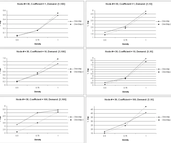
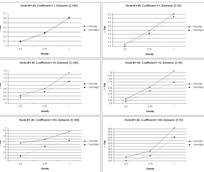
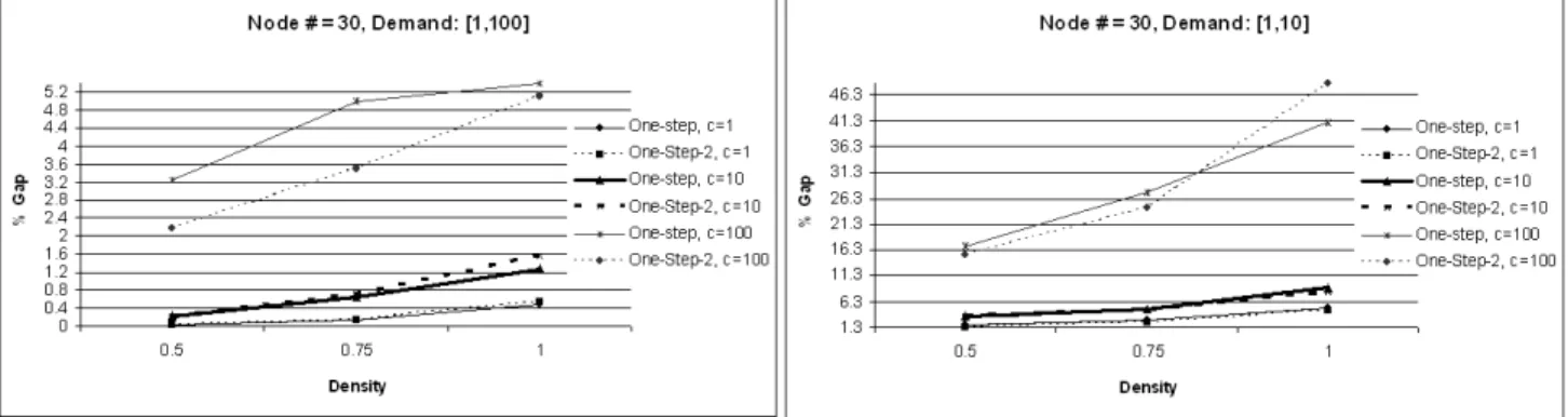
5.2.1 One-step and One-step-2 Algorithm Comparison . . . 35
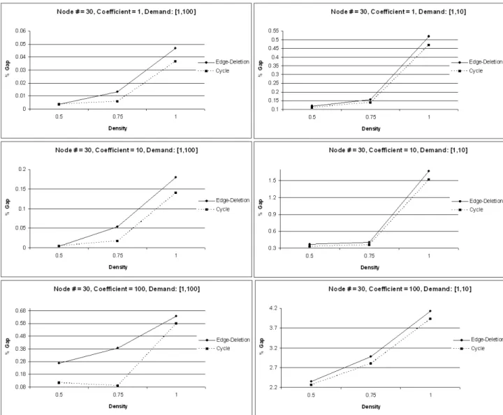
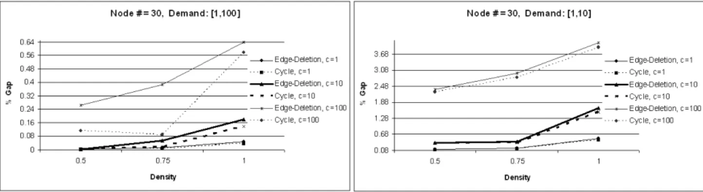
5.2.2 Edge Deletion Heuristic and Cycle Algorithm Comparison 36 5.2.3 Summary of Our Findings . . . 39
6 Conclusion 47
List of Figures
1.1 2-edge disjoint paths from s to t: Path 1: s-1-3-5-t, Path 2: s-2-4-t 5
4.1 An example which shows how Suurballe’s algorithm works . . . . 20
4.2 Steps of Edge Deletion Heuristic . . . 27
4.3 Steps of Edge Addition Heuristic . . . 28
4.4 An example for a single commodity i and j which shows how cycle algorithm works . . . 29
5.1 One-step and One-step-2 Algorithm Results for node # = 30 . . . 37
5.2 One-step and One-step-2 Algorithm Results for node # = 40 . . . 38
5.3 Edge Deletion Heuristic and Cycle Algorithm Results for node # = 30 and Comparison Results for One-step and One-step-2 Al-gorithms as the Construction Heuristics . . . 40
5.4 Edge Deletion Heuristic and Cycle Algorithm Results for node # = 40 and Comparison Results for One-step and One-step-2 Al-gorithms as the Construction Heuristics . . . 41
5.5 Edge Deletion Heuristic and Cycle Algorithm Results for node # = 30 . . . 42
LIST OF FIGURES x
5.6 Edge Deletion Heuristic and Cycle Algorithm Results for node # = 40 . . . 43
5.7 One-step and One-step-2 Algorithm: Results for All Test Instances 45
5.8 Edge Deletion Heuristic and Cycle Algorithm: Results for All Test Instances . . . 46
List of Tables
3.1 Notation . . . 13
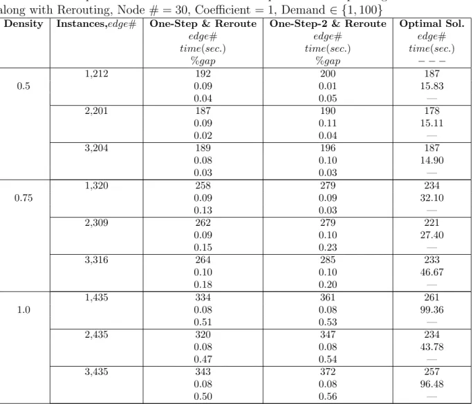
A.1 Computational Results of the One-Step and One-Step-2 Algorithm along with Rerouting, Node # = 30, Coefficient = 1, Demand ∈ {1, 100} . . . 53
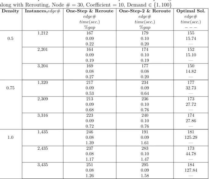
A.2 Computational Results of the One-Step and One-Step-2 Algorithm along with Rerouting, Node # = 30, Coefficient = 10, Demand ∈ {1, 100} . . . 54
A.3 Computational Results of the One-Step and One-Step-2 Algorithm along with Rerouting, Node # = 30, Coefficient = 100, Demand ∈ {1, 100} . . . 55
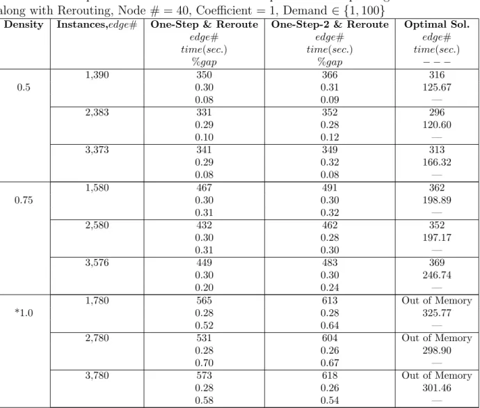
A.4 Computational Results of the One-Step and One-Step-2 Algorithm along with Rerouting, Node # = 40, Coefficient = 1, Demand ∈ {1, 100} . . . 56
A.5 Computational Results of the One-Step and One-Step-2 Algorithm along with Rerouting, Node # = 40, Coefficient = 10, Demand ∈ {1, 100} . . . 57
A.6 Computational Results of the One-Step and One-Step-2 Algorithm along with Rerouting, Node # = 40, Coefficient = 100, Demand ∈ {1, 100} . . . 58
LIST OF TABLES xii
A.7 Computational Results of the One-Step and One-Step-2 Algorithm along with Rerouting, Node # = 30, Coefficient = 1, Demand ∈ {1, 10} . . . 59
A.8 Computational Results of the One-Step and One-Step-2 Algorithm along with Rerouting, Node # = 30, Coefficient = 10, Demand ∈ {1, 10} . . . 60
A.9 Computational Results of the One-Step and One-Step-2 Algorithm along with Rerouting, Node # = 30, Coefficient = 100, Demand ∈ {1, 10} . . . 61
A.10 Computational Results of the One-Step and One-Step-2 Algorithm along with Rerouting, Node # = 40, Coefficient = 1, Demand ∈ {1, 10} . . . 62
A.11 Computational Results of the One-Step and One-Step-2 Algorithm along with Rerouting, Node # = 40, Coefficient = 10, Demand ∈ {1, 10} . . . 63
A.12 Computational Results of the One-Step and One-Step-2 Algorithm along with Rerouting, Node # = 40, Coefficient = 100, Demand ∈ {1, 10} . . . 64
A.13 Computational Results of the Edge-Deletion Heuristic and Cycle Algorithm Applied After One-Step-2 Algorithm, Node # = 30, Coefficient = 1, Demand ∈ {1, 100} . . . 65
A.14 Computational Results of the Edge-Deletion Heuristic and Cycle Algorithm Applied After One-Step-2 Algorithm, Node # = 30, Coefficient = 10, Demand ∈ {1, 100} . . . 66
A.15 Computational Results of the Edge-Deletion Heuristic and Cycle Algorithm Applied After One-Step-2 Algorithm, Node # = 30, Coefficient = 100, Demand ∈ {1, 100} . . . 67
LIST OF TABLES xiii
A.16 Computational Results of the Edge-Deletion Heuristic and Cycle Algorithm Applied After One-Step-2 Algorithm, Node # = 40, Coefficient = 1, Demand ∈ {1, 100} . . . 68
A.17 Computational Results of the Edge-Deletion Heuristic and Cycle Algorithm Applied After One-Step-2 Algorithm, Node # = 40, Coefficient = 10, Demand ∈ {1, 100} . . . 69
A.18 Computational Results of the Edge-Deletion Heuristic and Cycle Algorithm Applied After One-Step-2 Algorithm, Node # = 40, Coefficient = 100, Demand ∈ {1, 100} . . . 70
A.19 Computational Results of the Edge-Deletion Heuristic and Cycle Algorithm Applied After One-Step-2 Algorithm, Node # = 30, Coefficient = 1, Demand ∈ {1, 10} . . . 71
A.20 Computational Results of the Edge-Deletion Heuristic and Cycle Algorithm Applied After One-Step-2 Algorithm, Node # = 30, Coefficient = 10, Demand ∈ {1, 10} . . . 72
A.21 Computational Results of the Edge-Deletion Heuristic and Cycle Algorithm Applied After One-Step-2 Algorithm, Node # = 30, Coefficient = 100, Demand ∈ {1, 10} . . . 73
A.22 Computational Results of the Edge-Deletion Heuristic and Cycle Algorithm Applied After One-Step-2 Algorithm, Node # = 40, Coefficient = 1, Demand ∈ {1, 10} . . . 74
A.23 Computational Results of the Edge-Deletion Heuristic and Cycle Algorithm Applied After One-Step-2 Algorithm, Node # = 40, Coefficient = 10, Demand ∈ {1, 10} . . . 75
A.24 Computational Results of the Edge-Deletion Heuristic and Cycle Algorithm Applied After One-Step-2 Algorithm, Node # = 40, Coefficient = 100, Demand ∈ {1, 10} . . . 76
LIST OF TABLES xiv
A.25 Computational Results of the One-Step Algorithm, Node # = 30, Coefficient = 1, Demand ∈ {1, 100} . . . 77
A.26 Computational Results of the One-Step Algorithm, Node # = 30, Coefficient = 10, Demand ∈ {1, 100} . . . 78
A.27 Computational Results of the One-Step Algorithm, Node # = 30, Coefficient = 100, Demand ∈ {1, 100} . . . 79
A.28 Computational Results of the One-Step Algorithm, Node # = 40, Coefficient = 1, Demand ∈ {1, 100} . . . 80
A.29 Computational Results of the One-Step Algorithm, Node # = 40, Coefficient = 10, Demand ∈ {1, 100} . . . 81
A.30 Computational Results of the One-Step Algorithm, Node # = 40, Coefficient = 100, Demand ∈ {1, 100} . . . 82
A.31 Computational Results of the One-Step-2 Algorithm, Node # = 30, Coefficient = 1, Demand ∈ {1, 100} . . . 83
A.32 Computational Results of the One-Step-2 Algorithm, Node # = 30, Coefficient = 10, Demand ∈ {1, 100} . . . 84
A.33 Computational Results of the One-Step-2 Algorithm, Node # = 30, Coefficient = 100, Demand ∈ {1, 100} . . . 85
A.34 Computational Results of the One-Step-2 Algorithm, Node # = 40, Coefficient = 1, Demand ∈ {1, 100} . . . 86
A.35 Computational Results of the One-Step-2 Algorithm, Node # = 40, Coefficient = 10, Demand ∈ {1, 100} . . . 87
A.36 Computational Results of the One-Step-2 Algorithm, Node # = 40, Coefficient = 100, Demand ∈ {1, 100} . . . 88
LIST OF TABLES xv
A.37 Computational Results of the One-Step-2 Algorithm, Node # = 30, Coefficient = 1, Demand ∈ {1, 10} . . . 89
A.38 Computational Results of the One-Step-2 Algorithm, Node # = 30, Coefficient = 10, Demand ∈ {1, 10} . . . 90
A.39 Computational Results of the One-Step-2 Algorithm, Node # = 30, Coefficient = 100, Demand ∈ {1, 10} . . . 91
A.40 Computational Results of the One-Step-2 Algorithm, Node # = 40, Coefficient = 1, Demand ∈ {1, 10} . . . 92
A.41 Computational Results of the One-Step-2 Algorithm, Node # = 40, Coefficient = 10, Demand ∈ {1, 10} . . . 93
A.42 Computational Results of the One-Step-2 Algorithm, Node # = 40, Coefficient = 100, Demand ∈ {1, 10} . . . 94
Chapter 1
Introduction
Networks are being used in many settings to model and solve problems. A num-ber of problems that can be found in everyday life using networks are: Finding shortest paths, designing telecommunications networks, speeding up Internet, balancing the traffic on highways etc. Since the 90’s, an increasing number of telecommunications networks are being used. Especially, with the vast devel-opment of the Internet, and the need to transmit more data, design of surviv-able and properly capacitated networks have become imperative. Survivability is a keyword for today’s telecommunications networks due to the domination of telecommunications systems that have invaded consumers’ lives in every way. Hence, survivability is a critical design constraint for high-speed networks that satisfy the users. There are different types of protection schemes. However, the general idea is to connect source and destination pairs with more than a single path. By this way, if a failure on a path occurs another path can become active and the data transfer to the destination can be made safely. Equipment failures may occur due to construction or due to destructive natural events, such as earth-quakes, tsunamis, tornadoes etc. Since, repairing an equipment in a short time may not be possible, the use of another path during the mending of the failure will be necessary for the transfer of data between the source and the destination to continue.
How to choose the paths between source and destination pairs depends on the 1
CHAPTER 1. INTRODUCTION 2
severity of the survivability requirement. In general, node or link failures may occur so the paths can be either node-disjoint or edge-disjoint. Any number of disjoint paths can be considered from a source to a destination. But, finding and using disjoint paths is costly therefore a balance between survivability and total costs needs to be considered. In the literature two types of paths are referred to; primary(working) and secondary(backup) paths and most research focuses on the recovery from a single link or node failure. In other words, one failure is repaired before another failure occurs. Nonetheless, multiple failures in a realistic network may occur but this subject is beyond the scope of this thesis.
There are two types of protection schemes for using primary and secondary paths as survivability measures; dedicated protection and shared protection. In dedicated protection, a spare capacity is available such that if a destination point suffers a failure due to the spare capacity it is guaranteed that there will be avail-able resources to recover from the failure, assuming that the secondary resources have not failed. There are two types of categories of dedicated protection. In 1+1 dedicated protection, both the primary and the secondary path is active and the circuitry in the network chooses the better connection. On the contrary, in 1:1 dedicated protection only the primary path is active until a failure occurs in the network only then the secondary path is used. After the failure is overcome the primary path can be used again or the connection may continue to use the secondary path. The advantage of 1+1 dedicated protection is that the recovery from a failure can be nearly immediate. But, 1:1 dedicated protection is slower since the transmit must start over from the secondary path. Since 1+1 dedicated protection has both the primary and secondary paths active this type of approach requires more equipment which may be costly. For both 1+1 and 1:1 dedicated protection a spare capacity is needed which is considered as a downside of the dedicated protection scheme due to its cost. Shared dedication protection ad-dresses this downside by making the spare capacity available for more than one primary path. There is a restriction to which primary paths can share the spare capacity; they cannot have links or nodes in common.
While finding node-disjoint or edge-disjoint paths the total costs incurred by using the edges are considered. The edges have costs such that if 1 unit of demand
CHAPTER 1. INTRODUCTION 3
is sent through that edge the cost of that specific edge is added to the total cost. This is called the minsum problem which consists of finding k disjoint paths between two distinct nodes, a source and a destination such that the sum of the cost of the routes is minimum [5]. A polynomial running time algorithm developed for the edge-disjoint problem by Suurballe and Tarjan [12] solves the problem of finding 2-edge disjoint paths to optimality when the objective is the minimization of the sum of the costs of the used edges on both paths. However, Suurballe’s algorithm finds an optimal solution for only a single source and destination pair and when there is a single cost for each edge. According to the requirements of survivability and the objective function the problem can become NP-hard which causes the researchers to focus on different heuristic algorithms. In many real life problems which fall into the category of survivable network design there is a relationship between the two costs cp(e), cs(e) for each edge e, where the former
cost is used to compute the cost of a primary path while the latter is used for secondary path computation. This relationship is typically characterized in terms of a coefficient α such that 0 < α < 1 and cs(e) = αcp(e). However, the costs
cp(e), cs(e) can also be arbitrary. For the special case of cs(e) = αcp(e) for all
edges e, the problem of minimizing the total costs incurred is known to be NP-hard for directed graphs, i.e. graphs in which links have directions. This result holds whether the paths are required to be node or edge disjoint[3]. The node-disjoint and edge-node-disjoint paths problem for undirected graphs is also known to be NP-hard according to Xu et al. [14]. However, Bhatia et al. show that Xu et al.’s proof for the edge-disjoint problem in undirected graphs is flawed.
Other than the minsum problem, there is also a min-max version of the prob-lem. This problem minimizes the cost of the most expensive of the selected routes. Min-max version is much more difficult, Li et al. [9] showed that the min-max problem is strongly NP-complete even when k = 2 for the four possible variants of the problem; edge-disjoint, node-disjoint and the network is either directed or undirected.
In this thesis our aim is to solve a network design problem with requirements that define the survivability level along with different cost structures while min-imizing the total cost. We seek 2-edge disjoint paths for every possible origin
CHAPTER 1. INTRODUCTION 4
destination pair. We are given a graph G = (V, E), where V represents the node set and E represents the edge set. There is a a fixed cost, i.e., a cost for opening(or activating) an edge and two variable costs for an edge. Fixed cost is incurred once if edge is used. Two variable costs are costs for sending 1 unit of flow from that edge. There are two variable costs since one of the costs ce1ij is incurred if that edge {i, j} ∈ E is used along a primary path for a source-destination pair and the other cost ce2
ij is incurred if edge {i, j} ∈ E is used along a secondary path for
a source-destination pair. These two costs are also referred to as dual edge costs since there are two costs for each edge. We assume that the relationship between primary and secondary path costs is cs(e) = 1/2cp(e). In the literature, the cost
of using secondary paths is generally accepted as lower than their primary coun-terparts. This is because in normal circumstances the primary paths are used and only if some damage occurs in a primary path the secondary path is utilized for a source-destination pair. Any source-destination pair has a demand that needs to be satisfied. Throughout this thesis all possible source and destination pairs are assumed to exist. Figure 1.1 represents 2-edge disjoint paths for a source-destination pair, s − t. The first path is s → 1 → 3 → 5 → t and the second path is s → 2 → 4 → t. One may notice that there are only 2-edge disjoint paths from s to t hence, for any k > 2 this example will be infeasible. However, more than 1 different pair of edge-disjoint paths can be found. For example, the first path can be s → 1 → 3 → t and the second path can be s → 2 → 4 → 5 → t.
The rest of the thesis is organized as follows. Chapter 2 contains the literature review for survivable network design. In Chapter 3 an IP model which solves the 2-edge disjoint network problem with fixed and dual edge costs is presented. In Chapter 4, the specific details of the algorithms used to solve the problem are explained. In Chapter 5, the numerical results obtained from both the IP model and the algorithms are provided along with interpretations of the results. Finally, the thesis is summarized in Chapter 6 and possible future work is also discussed. For detailed numerical results the reader can review the Appendix.
CHAPTER 1. INTRODUCTION 5
Chapter 2
Literature Review
Survivability has become a major issue in telecommunications networks with the emerging need to transfer more data compared to earlier decades. Consumers desire a satisfying service that is without failure at all times. This requirement can be met via utilizing more than one route between a source and a destination pair to transfer data. Having an additional route, referred to as the back up or secondary path will provide a protection against a failure caused by a destruction in the primary path. By assumption a single node or link failure can happen. Therefore, if a problem occurs in transferring data that uses the primary path automatically the data transfer is continued by utilizing the secondary path until the complication in the primary path is fixed. To use the secondary path without any difficulties the primary and secondary path must be node or edge disjoint (having no common nodes or no common edges) that is, if one of the paths is out of order the other one will be ready to continue the data transfer.
The problem of finding “disjoint paths” is being studied since late 1950’s. De-velopments in MIP models, heuristic and exact algorithms can be seen throughout five decades. Research related to finding “disjoint paths” is divided according to different constraints since several types of equipment failure may occur in a net-work and interrupt traffic along paths. Hence, one of the major responsibilities of “disjoint paths” between a given source and sink is to increase reliability in communication networks. However, increasing reliability “too much” may be
CHAPTER 2. LITERATURE REVIEW 7
costly according to given network parameters. Therefore, a compromise between reliability and total cost needs to be achieved for a desirable output. Given a brief description of the general problem, the following paragraphs analyze the literature on “disjoint paths” in more depth.
In Suurballe’s paper [13] the problem of finding K node-disjoint paths with minimum total cost is presented. The total cost includes the summation of indi-vidual arc lengths used on paths between a source and a destination. Suurballe [13] describes a labeling algorithm involving K shortest path iterations. The idea presented by the author gives a polynomial time algorithm. Furthermore, with slight modifications as discussed in [12] the algorithm can also be used for finding edge-disjoint paths. Bhandari’s algorithm [2] which is a slight variation of Suur-balle’s algorithm also achieves the same results as SuurSuur-balle’s algorithm. Both Suurballe’s algorithm and Bhandari’s algorithm provide optimal results to the problem of finding a pair of edge-disjoint paths for a single source and destina-tion pair. The problem solved by Suurballe and Bhandari differ from our problem in several ways. First of all, we assume that all possible source and destination pairs exist in a given graph G. In addition, we consider two different path costs ce1ij and ce2ij for each edge {i, j} and fixed cost fij of activating an edge {i, j}.
Li et al. [10] consider a different problem compared to Suurballe since for a network G = (V, E) with source and sink nodes there are k different costs on every edge. Li et al. describe their problem as a minsum problem, where jth edge-cost
is associated with the jth path. They analyze several variants of the problem;
node-disjoint or edge-disjoint problems with directed or undirected networks. Li et al. claim that all four versions of the problem are NP-complete even when k = 2, for arbitrary primary and secondary path costs, however, Bhatia et al. [3] show that when, ce1
ij < ce2ij, Li et al.’s. NP hardness results do not extend
to this case. Li et al. present polynomial time heuristics and an algorithm for their proposed problem. The first heuristic they describe is a heuristic in which a function f of the k costs on each arc that “averages”’ the individual costs is defined. However, this “averages”’ concept is a function determined by the users of the algorithm so it may or may not be the same as the customary meaning of taking the average of k numbers. After computing this function f of k different
CHAPTER 2. LITERATURE REVIEW 8
costs for each arc a Minimum Cost Network Flow (MCNF) problem is solved such that the supply at the source node is k, the demand at the sink node is k, all other nodes have supply/demand equal to 0 and edges have capacity of 1. The second heuristic discussed in the paper arranges the edge costs according to the customary meaning of average, so it takes the average of the k different costs without creating a function f . Although Li et al. consider different path costs for edges their problem is fundamentally different from our problem since they do not consider fixed costs for activating edges.
Bhatia et al. [3] point out that the cost metric used for primary and secondary paths differ in some settings and in others they are somehow related to each other. More precisely, one of the costs may be a multiple of the other. The problem considered by Bhatia et al. is to find a pair of edge or node-disjoint paths of minimum cost where the costs of primary path is the total cost of the edges used on the paths while the cost for the secondary path is α times the sum of the cost of the links used on the path, where α < 1. This study is of great importance to this thesis where α = 1/2 for all of the test instances that are present in Chapter 5. Bhatia et al. argue that a simple algorithm achieves an approximation ratio of O(1/α) for the proposed problem. They also consider the four versions of the problem that are previously described in the above paragraph. The approximation algorithm they mention is Suurballe’s algorithm which runs in polynomial time. They prove that this algorithm is a 1/2 + 1/α approximation algorithm for their problem. They conclude by saying that if α is a fixed constant, as in this thesis, the hardness of the problem is still an open question. The problem that Bhatia et al. consider is the closest one to our problem in survivable network design literature. However, like other papers they do not consider fixed costs for activating edges.
A recent study conducted by Gomes et al. [5] like Li et al. [10] also analyzes the problem of calculating k disjoint paths from a source to a destination (two distinct nodes) in which there are k arbitrary costs on every edge and the total cost is minimized. Even when k = 2 this problem is NP-complete since the costs on edges are arbitrary. The authors refer to the networks as dual arc cost networks when k = 2. They propose an exact algorithm that finds 2 disjoint
CHAPTER 2. LITERATURE REVIEW 9
paths for source and destination pairs when the network has dual arc costs. The exactness of the algorithm they describe results from the fact that it allows the calculation of optimal solutions by using a condition to satisfy the optimality. The algorithm is based on calculating upper and lower bounds on the optimal cost. Two alternative problems can also be solved by slightly modifying their proposed algorithm. These problems are finding node-disjoint paths and disjoint paths with length constraints. The authors claim that their exact algorithm can solve any instance to optimality if memory and CPU times were unlimited. They present test instances with up to 1000 nodes and when the number of arcs are 3 or 4 times the number of nodes in the network. The worst case complexity of the algorithm is O(n3(u + v) + n(u + v)2), where n is the number of nodes and u + v is the number of generated shortest paths. The study presented by Gomes et al. in [5] is an extension to ideas presented in [4]. Although the algorithms provided in the two papers differ, the basic approach used to find the optimal solutions remains the same. The exact algorithm presented by Gomes et al. [5] is not utilized in this thesis due to its high complexity and memory usage. In addition, the algorithm described by the authors do not take into consideration fixed costs for activating edges.
Ho et al. [7] propose an Integer Linear Program (ILP) and two heuristics called Iterative Two-Step-Aprroach (ITSA) and Maximum Likelihood Relaxation (MLR) to solve the least-cost primary and secondary path-pair (in terms of the sum of the total cost). The authors use the shared protection scheme while solving the problem. Recall that in shared protection scheme a spare capacity is available such that if a destination point suffers a failure due to the spare capacity it is guaranteed that there will be available resources to recover from the failure, assuming that the secondary resources have not failed. In contrast to dedicated protection scheme this spare capacity is available for more than one primary path assuming that the primary paths in consideration do not share a link or a node. The ITSA heuristic enumerates and inspects all of the k-shortest paths as the primary path. Although ITSA provides better results in terms of the proximity to the optimal solution, the computational complexity becomes a bottleneck for larger problems in terms of node or link numbers. The other
CHAPTER 2. LITERATURE REVIEW 10
heuristic, MLR is a modified version of the Dijkstra’s algorithm [1] and yields polynomial time complexity. To explain it in more detail, MLR considers finding the secondary path during the calculations for finding the primary path. However, since MLR yields a polynomial time complexity the results obtained from it are not as satisfying as ITSA’s computational results. Networks with up to 100 nodes have been tested in the paper.
Another version of finding disjoint paths problem is to maximize the number of disjoint paths between a source and a destination. An extension to this problem is that length of every path is bounded by a given value, p. Itai et al. [8] analyze the complexity of this problem, while Perl and Ronen [11] present a polynomial time heuristic algorithm for any given bound value, p. For the test instances used in the paper, they prove that when p ≤ 5 optimal solutions are found and when p ≥ 5 solution values are in proximity to the optimal solution.
In addition to minimizing the cost of finding disjoint paths for single source and destination problems, several different source and destinations can also be added to the problem. However, having several source and destinations increases the complexity of the problem. Depending on the context of the problem there may be several destination points and one single source or vice versa. But any number of source and destination pairs is also possible.
One other problem differing from the previously mentioned settings is pre-sented by Guruswami et al. in [6]. The specific problem at hand is finding a maximum number of length bounded edge-disjoint paths between any given source and destination pairs. The authors show an analysis of the approximabil-ity of the proposed problem. Having presented their analysis, an O(√m) time approximation algorithm to solve the maximum edge-disjoint path problem is also provided.
The contribution of this thesis to the survivable network design literature is as follows: A new 2-edge connected network design problem is introduced. The task is to find 2-edge disjoint paths for every possible source to destination in the presence of fixed costs for edges and different routing costs for primary and secondary paths. First of all, the costs of primary and secondary paths
CHAPTER 2. LITERATURE REVIEW 11
are different but related to each other since, ce1
ij = 2ce2ij (primary path costs is 2
times the secondary path costs). Although there are are some studies on different path costs for edges, as Bhatia et al. [3] point out when αce1
ij = ce2ij and α is a
constant the question of whether the problem is NP-hard or not is still an open question. However, in addition to routing costs, ce1ij and ce2ij, we also consider fixed costs fij for each edge {i, j} ∈ E.
Chapter 3
Mathematical Model
In this section the IP model for our problem, namely, the Survivable Network Design Dedicated Protection (SND DP) is introduced along with some analysis. Given a network, the task is to find 2-edge disjoint paths for every commodity in the network such that primary and secondary paths have different edge costs and a fixed cost for opening an edge for usage is encountered. Although a network is assumed to be available at hand, using an edge for the first time or activating it requires a fixed cost. The outcome of the model will produce two paths that have no common edges for each commodity. The objective is to minimize the total costs.
Given a graph G = (V, E) with edge costs ce1
ij, ce2ij, fij and commodity set
K, the survivable network design problem discussed in this thesis is to find a minimum cost subgraph of G such that between every pair in the commodity set K, there are at least 2-edge disjoint paths.
Cost ce1
ij is the cost of routing a unit flow on edge {i, j} ∈ E on the primary
path and cost ce2
ij is the cost of routing a unit flow on edge {i, j} ∈ E on the
secondary path. Cost fij is the fixed cost of activating edge {i, j} ∈ E. For each
commodity k ∈ K, s(k) ∈ V is the origin, t(k) ∈ V is the destination, and d(k) is the demand between the origin and destination. For quick reference to the notation used in this chapter the reader may look at Table 3.1.
CHAPTER 3. MATHEMATICAL MODEL 13
G : Given graph
V : Vertex set in graph G E : Edge set in graph G K : Commodity set ce1
ij : Unit routing cost of edge {i, j} ∈ E for primary path
ce2ij : Unit routing cost of edge {i, j} ∈ E for secondary path fij : Fixed cost of activating edge {i, j} ∈ E
s(k) : Origin for commodity k ∈ K t(k) : Destination for commodity k ∈ K d(k) : Demand for commodity k ∈ K
Table 3.1: Notation
We use the following decision variables in our model:
xpk
ij is the decision variable to keep track of which edge belongs to the
pri-mary path of the specific commodity at hand. Similarly, xsk
ij is the decision
variable which holds the edges belonging to the secondary path for each com-modity. The last decision variable, yij is necessary to keep track of the edges that
are −opened− in order to add the fixed costs of opening an edge to the objective function value. xpk ij =
1, if edge {i, j} ∈ E is used in the direction f rom i to j on the primary path of commodity k ∈ K
0, otherwise xsk ij =
1, if edge {i, j} ∈ E is used in the direction f rom i to j on the secondary path of commodity k ∈ K
0, otherwise
yij =
(
1, if edge {i, j} ∈ E is used 0, otherwise
CHAPTER 3. MATHEMATICAL MODEL 14 min X {i,j}∈E fijyij+ X k∈K X {i,j}∈E (ce1ijd(k)(xpkij+xpkji)+ce2ijd(k)(xskij+xskji)) (3.1) s.t. X j:{i,j}∈E xpkij− X j:{i,j}∈E xpkji= 1, if i = s(k) ∀ k ∈ K, ∀ i ∈ V −1, if i = t(k) ∀ k ∈ K, ∀ i ∈ V 0, otherwise (3.2) X j:{i,j}∈E xskij− X j:{i,j}∈E xskji = 1, if i = s(k) ∀ k ∈ K, ∀ i ∈ V −1, if i = t(k) ∀ k ∈ K, ∀ i ∈ V 0, otherwise (3.3) xpk ij+ xpkji+ xskij+ xskji ≤ yij ∀k ∈ K, ∀ {i, j} ∈ E (3.4) xpk ij, xskij ∈ {0, 1} ∀k ∈ K, ∀ {i, j} ∈ E (3.5) yij ∈ {0, 1} ∀ {i, j} ∈ E (3.6)
Constraints (3.2) and (3.3) are flow balance constraints. Here since we are searching for two paths, for each commodity, two sets of flow balance equations are written; one for the primary path (3.2) and one for the secondary path (3.3).
However, finding two paths for each commodity is not adequate since the task is to find two −disjoint− paths. Therefore, an edge {i, j} ∈ E can only be used in one path; primary or secondary path for each commodity. Constraint (3.4) satisfies this request by bounding the number of times a commodity can use an edge. This constraint also opens edge {i, j} ∈ E if that edge has been used by a commodity in either its primary or secondary path.
The first part of the summation in the objective function; X
{i,j}∈E
CHAPTER 3. MATHEMATICAL MODEL 15
calculating the total costs incurred due to the activation of the edges. The second part of the summation; X
k∈K
X
{i,j}∈E
(ce1ijd(k)(xpkij+ xpkji) + ce2ijd(k)(xskij + xskji)) is necessary for calculating the total routing costs. The demands are used in this calculation since, the variable costs ce1ij and ce2ij are costs for routing a unit demand.
As observed in the above given model, constraints (3.2) and (3.3) are flow balance constraints. Hence, if the edge set to be used is given, i.e., yij values are
fixed, the problem boils down to finding 2-edge disjoint paths for each commod-ity. This implies that if the fixed cost fij values are small in value to routing
costs ce1ij and ce2ij the problem becomes easier. Furthermore, this problem is a Minimum Cost Network Flow (MCNF) problem if there were single edge costs cij
for finding 2-edge disjoint paths. We refer to this problem as Single Commodity Routing Problem (SCRP). The idea of using MCNF is important since Suur-balle’s algorithm [12] takes its origins from this model. The detailed explanation for Suurballe’s algorithm is presented in Chapter 4.
We define, xk ij =
1, if edge {i, j} ∈ E is used in the direction f rom i to j on a path f or commodity k ∈ K
0, otherwise
Now, we can model the SCRP as follows:
min X k∈K X {i,j}∈E cijxkij s.t. X j:{i,j}∈E xkij − X j:{i,j}∈E xkji = 2, if i = s(k) ∀ k ∈ K, ∀ i ∈ V −2, if i = t(k) ∀ k ∈ K, ∀ i ∈ V 0, otherwise
CHAPTER 3. MATHEMATICAL MODEL 16
0 ≤ xk
ij ≤ 1 ∀k ∈ K, ∀ {i, j} ∈ E
The number of commodities used in SND DP severely enlarges the problem in terms of the memory that is used. As the number of nodes increases, so does the number of commodities. This is because by assumption, in this thesis all of the possible combinations of source and destination pairs exist. In addition, the possible density of the graph; the amount of edges that are available, also effects the memory usage.
Differing edge costs for primary and secondary paths are other factors that make the problem harder (Recall that Suurballe and Tarjan’s algorithm solves to optimality the 2 edge-disjoint problem with single routing costs for edges for a single commodity [12]). Throughout this thesis the assumption is that the relationship between the routing costs is: 1/2ce1ij = ce2ij.
In the next chapter, different consruction and improvement heuristics are expressed.
Chapter 4
Heuristic Algorithms
In our problem, we find 2-edge disjoint paths between source and destination pairs. The objective is to minimize the total costs. These costs include primary and secondary path routing costs and fixed costs for opening edges. Recall that primary path costs is 2 times the secondary path costs.
To solve our problem, in this chapter, we make use of several algorithms. Firstly, Suurballe’s algorithm is described since it is one of the basic algorithms utilized in the heuristic algorithms that are illustrated in this section. Afterwards two of the consrtuction heuristics, namely, the two-step and one-step algorithm are described. These algorithms find initial feasible solutions for our problem. Finally, before concluding this chapter we explain improvement methods that can be applied to both of the construction heuristics. The improvement methods are referred to as the IP based heuristic, edge deletion heuristic, edge addition heuristic and cycle algorithm. These methods are explained in depth in section Improvement Heuristics.
CHAPTER 4. HEURISTIC ALGORITHMS 18
4.1
Suurballe’s Algorithm
Given a graph G = (V, E), with single edge costs cij for each edge {i, j} ∈ E,
a source node s, and destination node d, the survivable network design problem solved by Suurballe finds 2-edge disjoint paths between s and d while minimizing the total cost of these 2 paths. Cost cij is the cost of routing a unit flow on edge
{i, j} ∈ E.
Suurballe and Tarjan [12] describe Suurballe’s algorithm that solves the 2-edge disjoint paths problem. The method is based on the generic algorithm explained in [13] which is for finding node-disjoint paths. The altered version of the algo-rithm, which solves the 2-edge disjoint paths problem, runs in O(m log1+m/nn) time and O(m) space, where m is the number of edges and n is the number of nodes given in a graph G.
The algorithm starts by finding a shortest path tree from node s to all other nodes using Dijkstra’s algorithm [1]. Afterwards, the original graph G is altered by changing the cost values of the edges, while everything else remains the same. The new edge costs for an edge {u, v} are calculated as follows:
πu,v = cu,v+ ds,u− ds,v, where cu,v represents the original cost values of the edges,
ds,u is the shortest path distance from node s to u and ds,v is the shortest path
distance from node s to v. The new edge costs are simply the reduced costs from LP duality when the LP model in discussion is the relaxation of SCRP. Then, the edges’ directions used in the shortest path from node s to node d are reversed. The shortest path from node s to node d is calculated again using new edge costs and new edge directions for the edges found on the previous shortest path. After removing the links that appear (in opposite direction) in both the original shortest s − d path and the latter shortest path s − d tree 2-link disjoint paths between nodes s and d can be easily constructed. The pseudo-code of the algorithm can be found in Algorithm 1.
For a deeper understanding of the algorithm one can analyze the example in Figure 4.2. In this example 2-edge disjoint paths from node 0 to node 5 are to be found. Numbers next to edges which are inside rectangles represent edge
CHAPTER 4. HEURISTIC ALGORITHMS 19
Algorithm 1 Suurballe
Compute the shortest-path tree rooted at node s using Dijkstra’s algorithm [1]. Let ds,u denote the shortest-path distance from node s to node u.
Transform the original graph G to an auxiliary graph G0 as follows: Node and links are kept unchanged.
The cost of each link {u, v} in G0 is defined by πu,v = cu,v+ ds,u− ds,v, where πu,v denotes the
cost of link {u, v} in graph G0 and cu,v denotes the
cost of link {u, v} in graph G.
Reverse the directions of the links along the shortest path from node s to node d.
Compute the shortest path from node s to node d in graph G0.
The shortest path between nodes s and d in G(G0) is denoted as P (P0). Remove the links appearing in both P and P0
(in opposite direction), all the other links in P and P0
form a cycle when ignoring their directions. Two link-disjoint paths between nodes s and d are found from the cycle.
costs. The dashed lines show the shortest-path tree rooted at node 0. The shortest path from node 0 to node 5 is P = 0 → 1 → 4 → 5. After completing the transformation of the graph from G to G0, the shortest path between nodes 0 and 5 is P0 = 0 → 3 → 4 → 1 → 2 → 5, which can be observed in part (b) of the figure. After removing the arcs (1, 4) and (4, 1), the 2-edge disjoint paths 0 → 3 → 4 → 5 and 0 → 1 → 2 → 5 are found and shown in part (c) of the figure.
4.2
Construction Heuristics
In this section, the construction heuristics that utilize both Dijkstra’s and Suur-balle’s algorithm are described. These heuristics find initial feasible solutions.
4.2.1
Two-Step Algorithm
The basic idea used in the two-step algorithm is the application of Dijkstra’s al-gorithm [1] using single link costs that are equal to primary path costs, ce1ij. For
CHAPTER 4. HEURISTIC ALGORITHMS 20
CHAPTER 4. HEURISTIC ALGORITHMS 21
each commodity Dijkstra’s shortest path algorithm is applied once to construct the primary path. Then, the edges used in the primary path are temporarily deleted from the network so that the second application of the Dijkstra’s algo-rithm does not use these edges. By this way, the secondary path is also found assuming 2-edge disjoint paths exist for that commodity. This process is done as if only the particular commodity at hand exists, i.e., the total costs for each commodity are calculated seperately without considering active or inactive edges. Thus, the fixed costs are not included in the total costs. Afterwards the com-modity in discussion is placed in a commodities array which holds the total costs (primary path cost + secondary path cost) for that commodity. Finally, when the total cost calculation for each commodity is completed the values in this array are sorted according to descending order of total costs for each commodity.
At the end of the above process the problem is solved again according to the order of commodities in the commodities array. However, in this case the fixed costs are also considered while finding total costs for each commodity. Fur-thermore, each commodity is not thought of seperately, i.e., after a commodity’s two paths are fixed and total costs are calculated the next commodity does not pay any fixed costs if it uses edges that were previously activated. Until all of the commodities in the commodities array are processed the assigment of paths continues. At the end a feasible solution is obtained.
To improve the feasible solution at hand, a “rerouting”’ procedure is also performed. In this procedure, only the edges which were activated during the above explained steps are used and the fixed costs are added to the total costs at the end of the algorithm. Basically, for every commodity two paths are found again assuming that only the active edge set provided by the above steps is available. Furthermore, if any of the edges which were activated as a result of the above process are not used during the rerouting procedure, they are left out of the active edge set and their fixed cost values are not included in total costs.
The important point to consider in this algorithm is the order of connection of the commodities. In other words, the key question is which commodity should be processed first since the primary and secondary paths constructed for that
CHAPTER 4. HEURISTIC ALGORITHMS 22
commodity become permanent. This is essential in terms of activating the edges. If the fixed cost values are large in value compared to routing costs ce1
ij and ce2ij
the order of activating edges becomes crucial in finding good solutions; solutions that are closer in value to the optimal solution.
A number of approaches have been considered in determining the order of commodities to be processed. One of these approaches calculates the total costs (objective value) for each commodity as if other commodities do not exist by using the two-step algorithm. However, during this calculation fixed costs are not included in the total costs; only routing costs are considered. Afterwards, the commodities are listed in descending values in terms of their total costs (This process is explained in the first paragraph). Hence, the commodity that gives the largest total cost is processed first by this approach and the commodity that gives the smallest total cost is processed last. Furthermore, this approach can also be applied multiple times by using a dynamic calculation technique. After processing the first commodity in the list, several edges are activated. By using this information the calculation of the total costs for each commodity can be made again and the new ordering will probably be different from the previous ordering since the activated edge set will be different after the first(in the list) commodity’s paths are made permanent. This dynamic calculation technique can be repeated as many times as |K| − 1 where |K| is the number of commodities. However, although the results provided by this dynamic calculation technique may be better compared to ordering the commodity list only once, the running times of the dynamic calculations will be much higher. Another approach is to randomly list the commodities. Unfortunately, the drawback of this approach is that the total cost found by using random listing can be very close to the optimal solution in some cases and in others far away from the optimal solution. The unstability of random listing makes this approach unfavorable.
After testing these approaches, we have decided to use the static listing of commodities. Calculating the total costs once for each commodity has better times compared to dynamic listing. Furthermore, several improvement methods have been discussed that will improve the quality of the solution and still obtain considerably less running times. As discussed above, the random listing approach
CHAPTER 4. HEURISTIC ALGORITHMS 23
has not been chosen due to its unstable results. The pseudo-code for the two-step algorithm that lists the commodities according to static listing and by following this list processes the commodities one by one can be found in Algorithm 2. Algorithm 2 Two-Step
for all k ∈ K do
Using Dijkstra’s algorithm (edge costs according to ce1
ij) calculate the
short-est(primary) path from source s(k) to destination t(k)
Temporarily delete the edges used on the primary path for commodity k from the given graph G
Using Dijkstra’s algorithm (edge costs according to ce2ij) calculate the short-est(secondary) path from source s(k) to destination t(k)
Place commodity k in commoditiesArray after calculating the total costs as primary path cost + secondary path cost
Sort the commoditiesArray in descending order of total costs for all k ∈ commoditiesArray do
Using Dijkstra’s algorithm calculate the shortest(primary) path from source s(k) to destination t(k) using the following costs for edges
if Edge has been activated before then Cost of edge = ce1ij
else if Edge has not been activated before then Cost of edge = ce1
ij + fij and activate edge e = {i, j}
Temporarily delete the edges used on the primary path for commodity k from the given graph G
Using Dijkstra’s algorithm calculate the shortest(secondary) path from source s(k) to destination t(k)
if Edge has been activated before then Cost of edge = ce2
ij
else if Edge has not been activated before then Cost of edge = ce2
ij + fij and activate edge {i, j}
Reroute and close unused edges
4.2.2
One-Step Algorithm
In one-step algorithm instead of the naive approach of merely using Dijkstra’s algorithm, Suurballe’s algorithm is utilized. The underlying process used in both algorithms; the one-step and two-step algorithms are the same. Both of the algorithms initially find the total costs for each commodity as if other commodities
CHAPTER 4. HEURISTIC ALGORITHMS 24
do not exist in the problem and a listing of the commodities is done according to descending order of total costs. The total costs include the routing costs; fixed cost values are not considered. Thus, the basic difference is the usage of Suurballe’s algorithm for one-step algorithm. At the very end of the one-step algorithm, a “rerouting”’ procedure is performed like the rerouting procedure explained in the two-step algorithm.
In addition to the importance of listing the commodities as explained previ-ously, one of the other crucial factors in using Suurballe’s algorithm is to deter-mine which costs will be used during the utilization of the algorithm. This is important since Suurballe’s algorithm assumes that only a single cost for an edge is available.
For the calculation of the initial total costs, the edge costs are arranged as primary path costs; ce1ij for the Suurballe’s algorithm. However, after the sorting of the commodities according to descending order of total costs is completed the former approach is altered. During the second application of Suurballe’s algorithm for each commodity, the edge costs remain as primary path costs (ce1
ij)
if that specific edge has not been activated before else, the cost of the edge becomes primary path costs (ce1ij) + fixed cost of that edge. Since by using the one-step algorithm we make the fixed cost (fij) values the important factors in
defining the paths, the solution tries to choose all of the edges with lower fixed costs (fij) if available. This makes the problem favor some edges over others.
By altering the edge costs the favoring of the edges can become more balanced. This can be achieved by considering the weight (wij) of an edge. The one-step
algorithm is altered to create the one-step version 2 algorithm by changing the edge costs. Instead of checking if an edge has been activated and arranging the costs to include the fixed costs if that edge has not been activated before a more complex method is used. In this method, during the second application of the Suurballe’s algorithm for each commodity the edge costs are arranged as primary path costs (ce1ij) + fixed cost (fij) / weight of edge (wij). The edge
weights(wij) are calculated during the first application of Suurballe’s algorithm
in the part before the commodities are sorted according to their total costs in the one-step algorithm. The edge weights(wij) for a particular edge {i, j} is equal
CHAPTER 4. HEURISTIC ALGORITHMS 25
to the amount of routing done throughout that edge. The routing amount for an edge is calculated by considering −how much− demand that edge carries. By cumulatively adding all of the demands that are carried by edge {i, j} we obtain the weight of edge {i, j}, wij. In compact form, the weight of an edge, wij is equal
to P
k∈K: k uses edge on primary path{i,j}dk +
P
k∈K: k uses edge on secondary path{i,j}1/2dk
.
Furthermore, the outcome of Suurballe’s algorithm is two paths. The decision of making which path to be primary and which path to be secondary is important in reducing the total costs as much as possible. Both of the alternatives are considered by assigning one path to be primary path and other to be secondary path and vice versa. The assignment which provides the lowest total cost is chosen and the activation of the edges are done accordingly. The pseudo-code for the one-step algorithm that processes the commodities according to static listing one by one can be found in Algorithm 3.
Algorithm 3 One-Step for all k ∈ K do
Using Suurballe’s algorithm (edge costs according to ce1
ij) calculate two paths
from source s(k) to destination t(k)
Make the path with the larger total cost value the secondary path and the other primary path for commodity k
Place commodity k in commoditiesArray after calculating the total costs as primary path cost + secondary path cost
Sort the commoditiesArray in descending order of total costs for all k ∈ commoditiesArray do
Using Suurballe’s algorithm calculate two paths from source s(k) to destina-tion t(k)
if Edge has been activated before then Cost of edge = ce1
ij
else if Edge has not been activated before then Cost of edge = ce1ij + fij and activate edge {i, j}
Assign one path to be primary path and other to be secondary path and vice versa.
Pick the arrangement with the lowest costs and change the activated edge information if necessary
Reroute and close unused edges
CHAPTER 4. HEURISTIC ALGORITHMS 26
this is because the computational results for the two-step algorithm are very poor when compared to one-step algorithm’s results. This is an implied result since the two-step algorithm eliminates all of the edges that are used on a primary path from a source to a destination in order to find a disjoint secondary path for the same pair. However, one-step algorithm utilizes Suurballe’s algorithm and in this algorithm the edges used on a primary path for a source and des-tination pair are not completely removed from the graph before calculating the secondary paths for the same pair. Instead, the edges utilized on the primary path’s directions(orientations) are reversed. Hence, merely using two applica-tions of Dijkstra’s algorithm provides a smaller subset of edges for the search of secondary paths compared to Suurballe’s algorithm.
4.3
Improvement Heuristics
In this section several improvement methods for the one-step and one-step ver-sion 2 algorithms are explained (These improvement methods can also be ap-plied to the two-step algorithm but no computational results are presented for the two-step algorithm due to the explanation made in the previous paragraph). One-step and one-step version 2 algorithms are constructive heuristics and essen-tially provide initial feasible solutions that can be further improved. All of the improvement methods can be applied to both of the algorithms.
4.3.1
IP Based Heuristic
IP based heuristic basically does what “rerouting”’ procedure does but it finds the optimal solution for the resulting active edge set that is found after the application of one of the construction heuristics. In other words, the active edge set is provided to the model described in Chapter 3 and the fixed costs are omitted from the objective function. After an optimal solution to this problem is found the edge set is checked for any edge that may have become inactive and only then the fixed cost values are calculated for the new active edge set and added to the
CHAPTER 4. HEURISTIC ALGORITHMS 27
Figure 4.2: Steps of Edge Deletion Heuristic
problem. Although IP based heuristic may provide better solutions compared to the “rerouting”’ procedure, the resource usage of IP based heuristic is much higher.
4.3.2
Edge Deletion
In this improvement all of the active edges provided by one of the construction heuristics are made inactive one by one and the problem is solved again for the same algorithm. After making an edge inactive the problem may become infeasible hence, in these situations the edge is reactivated without checking the total cost value. Furthermore, making an edge inactive may increase the previous total costs so, inactivating that edge is not favorable. An edge is made inactive only when the new solution to the problem with the new active edge set has smaller total costs compared to the previous costs and it provides a feasible solution. This improvement method can also be applied using GAMS with the model in Chapter 3. However, having to do as many iterations as the active edges provided by one of the algorithms can be very costly in terms of the running times. The reader can view Figure 4.2 for the steps of Edge Deletion Heuristic.
4.3.3
Edge Addition
Edge addition is the reverse of edge deletion. Inactive edges; edges that are not provided by the result of one of the construction heuristics are made active one by one. There is no infeasibility in this case since edges that were inactive are made active (the active edge set becomes larger) and the problem is solved again with
CHAPTER 4. HEURISTIC ALGORITHMS 28
Figure 4.3: Steps of Edge Addition Heuristic
the algorithm that had provided the inactive edges. If the total costs decrease, a new solution is found. Total costs can decrease in value if some other previously active edge has become inactive. However, if the total costs increase, the edge that was activated is inactivated once again. This process continues until all of the inactive edges have been activated once. The reader can view Figure 4.3 for the steps of Edge Addition Heuristic.
4.3.4
Cycle Algorithm
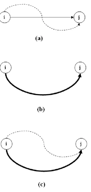
Having tested improvement heuristics that merely add or delete edges but do not combine both approaches we thought that we could unite these heuristics under the same algorithm. Therefore, in this section we describe the cycle algorithm that both removes and adds edges to a solution at a single iteration. The algo-rithm utilizes the one-step version 2 algoalgo-rithm. Essentialy an alternative cycle after obtaining a feasible solution for a source-destination pair is sought for. The steps of the cycle algorithm for a single source and destination pair; i and j can be observed in Figure 4.4. In part (a) edge {i, j} shows the primary path and the dashed curved line shows the secondary path for the i and j pair. This solution is obtained via the usage of one-step version 2 algorithm. In part (b), if possible, a third path is found such that no common edges between this path and primary and secondary paths exist. After closing edge {i, j}, we still have two paths for the i and j pair, as shown in part (c).
The algorithm starts by finding an initial feasible solution by applying the one-step version 2 algorithm. Afterwards, for every edge {i, j} in the activated edge set, E0 obtained via the initial feasible solution, edges in the primary and secondary paths from source i to j is removed. Dijkstra’s shortest path algorithm
CHAPTER 4. HEURISTIC ALGORITHMS 29
Figure 4.4: An example for a single commodity i and j which shows how cycle algorithm works
CHAPTER 4. HEURISTIC ALGORITHMS 30
is applied to the i and j pair. The edge costs are arranged according to the activated edge set E0, if an edge belongs to the edge set obtained from the initial feasible solution (E0) its cost is equal to primary path costs, ce1
kl, if an edge
belongs to the edge set of the original graph but has not been activated in the initial feasible solution (E − E0) its cost is equal to primary path costs (ce1kl) + fixed cost (fij) / weight of edge (wij) (wij is described in the previous section). If a
new shortest path from i to j is not found (no path exists) the algorithm continues with the next edge in the activated edge set, E0 else, edge {i, j} is inactivated and −rerouting− described in the two-step algorithm is applied once again. The cost arrangement for the edges is the same as the arrangement used for applying Dijkstra’s algorithm. If closing edge {i, j} provides a new feasible solution with improved costs then the edge stays inactive else the edge is reactivated. This process continues till there are no more edges to process in the initial activated edge set provided by the initial feasible solution. The pseudo-code for the cycle algorithm can be found in Algorithm 4.
Algorithm 4 Cycle
Run One-step version 2 algorithm
current cost is equal to the total cost returned by the algorithm for all e = {i, j} ∈ E0 do
Temporarily delete the edges used in primary and secondary paths for i(source) and j(destination) pair
Find a new shortest path from i to j using Dijkstra’s algorithm Using edge costs
if Edge e = {k, l} ∈ E0 then Cost of edge e = ce1kl
else if Edge e = {k, l} ∈ E − E0 then Cost of edge e = ce1
kl+ fij/wij
if a shortest path from i to j is found then inactivate e = {i, j}
Reroute using the same edge cost structure used for running Dijkstra’s algorithm
if new cost returned from rerouting < current cost then current cost = new cost
else if new cost returned from rerouting > current cost then activate e = {i, j}
CHAPTER 4. HEURISTIC ALGORITHMS 31
methods in this section, in Chapter 5 we take a look at the computational results provided by these algorithms and improvement methods.
Chapter 5
Numerical Results of Algorithms
In this chapter the algorithms and improvement methods described in Chapter 4 are tested on a computer with 2.6 GHz AMD Opteron 252 processor and 2 GB of RAM operating under the system CentOS (Linux version 2.6.9-42.0.3.ELsmp). Furthermore, in order to obtain the optimal solution values for the test instances, we solved the IP model presented in Chapter 3 by using GAMS 22.5 and CPLEX 11.0.0 on the same computer.
5.1
Test Instances
In this section the characteristics of the test instances are explained. The running times of the algorithms and improvement methods are effected differently accord-ing to particular aspects of the test instances. Increasaccord-ing the node number and edge numbers also increase the running times. In addition, the memory usage increases and in some test instances the computer runs out of memory. Fur-thermore, relationship between routing costs ce1
ij, ce2ij and fixed cost fij severely
effect the running times of the IP model. If the routing costs and fixed costs are in proximity of each other, the problem becomes easier so the running times decrease. However, if the routing costs and fixed costs are very different from each other and the fixed cost values are extremely higher than routing costs then
CHAPTER 5. NUMERICAL RESULTS OF ALGORITHMS 33
the running times severely increase. Therefore, a bound of 60 minutes is used for any test case and any method of solving the problem in this thesis.
5.1.1
Node Number (V )
The number of nodes selected for the test instances is 30 and 40. This choice is due to the memory restrictions of the mathematical model. Comparison of the optimal solution provided by the mathematical model and the total cost value obtained from the algorithms along with their improvements is impossible for larger instances when an optimal solution cannot be found. In these cases the lower bound provided by the IP model is used for comparison purposes.
5.1.2
Edge Number (E)
Edges are generated randomly according to three different density levels; 0.5, 0.75 and 1 respectively. Each corresponds to the probability of an edge appearing in the graph.
5.1.3
Primary and Secondary Path Costs (ce
1ijand ce
2ij)
Nodes are randomly selected from a 100 × 100 grid and the edge distances are simply calculated as the Euclidean distances between the points. This process is done for each edge of the network. The euclidean distance found is set as the secondary path costs (ce2ij) of each corresponding edge. To obtain the primary path costs, ce1
ij = 2ce2ij calculations are done for each edge of the network.
5.1.4
Fixed Cost (f
ij)
There are three components that make up a fixed cost; a random number, a co-efficient c and primary path costs (ce1ij).
CHAPTER 5. NUMERICAL RESULTS OF ALGORITHMS 34
fixed cost fij for some edge {i, j} = RandomN umber + c × ce1ij(primary path cost
of some edge (i, j))
The random number ∈ [0, 1000]. Coefficient c is either one of 1, 10 or 100 in different settings. Here the random number is assigned according to the geo-graphical conditions the fibers are installed. For example, having to install fibers underground and aboveground have different costs. The coefficient c is a param-eter for us to detect how the IP model and the algorithms behave when the range between fixed costs fij and routing costs ce1ij vary.
5.1.5
Demand (d)
Every possible combination of commodities is available according to the node number 30 or 40. However, a commodity with source node s and destination node d, and source node d and destination node s use the same primary and secondary paths. Hence, adding both demands and finding 2-edge disjoint paths from source node s to destination node d is adequate. Two demand value ranges are possible; either d ∈ [1, 10] or d ∈ [1, 100].
5.2
Results of Test Instances
In this section the results of the one-step and one-step version 2 algorithm are presented. Furthermore, a comparison between the edge deletion improvement heuristic and cycle algorithm is done. For detailed tables the reader may look at the Appendix. In the Appendix the running times along with the number of edges that were activated in the relevant algorithms are also presented.
The IP based heuristic results for the one-step algorithm have been tested. However, the running times are slow therefore, the “rerouting”’ procedure de-scribed in the construction heuristics is utilized instead. This improvement heuris-tic has not been used to test one-step version 2 algorithm due to its running times. The interested reader may take a look at the detailed results in the Appendix.