ISTANBUL BILGI UNIVERSITY
INSTITUTE OF SOCIAL SCIENCES
FINANCIAL ECONOMICS MASTER’S DEGREE PROGRAM
REVISITING THE OVERREACTION HYPOTHESIS:
EVIDENCE FROM ENERGY SECTOR
Kader VATANSEVER
116621005
Faculty Member, PhD Ebru REİS
ISTANBUL 2018
iii
ACKNOWLEDGMENTS
I would like to represent my sincere thanks to my supervisor, Dr. Ebru Reis, for her expertise, understanding, generous guidance and support made it possible for me to work on a topic that was of great interest to me. It was a great pleasure working with her.
I am also deeply grateful to my family for their supports, patience and love. Without their supports, it would be really hard to complete graduate education.
iv
TABLE OF CONTENTS
ACKNOWLEDGMENTS ... iii
FIGURE LIST ... vi
TABLE LIST ... vii
ABSTRACT ... x
ÖZET ... xi
INTRODUCTION ... 1
FIRST CHAPTER ... 2
EFFICIENT MARKET HYPOTHESIS, BEHAVIORAL FINANCE AND ANOMALIES ... 2
1.1. EFFICIENT MARKET HYPOTHESIS ... 2
1.1.1. Weak Form of Market Efficiency ... 2
1.1.2. Semi Strong Form of Market Efficiency ... 3
1.1.3. Strong Form of Market Efficiency ... 3
1.2. BEHAVIORAL FINANCE ... 4 1.3. MARKET ANOMALIES ... 4 1.3.1. Calendar Anomalies ... 5 1.3.2. Price Anomalies ... 5 SECOND CHAPTER ... 7 LITERATURE REVIEW ... 7 2.1. EVENT STUDY ... 7 2.1.1. Earning Announcements ... 8 2.1.2. Stock Splits ... 9
2.1.3. Annual Reports and Financial Statements ... 10
2.1.4. Merger and Acquisition... 11
2.2. OVERREACTION ... 12
THIRD CHAPTER ... 18
EMPIRICALLY TESTING THE OVERREACTION HYPOTHESIS ... 18
3.1. METHODOLOGY ... 18
3.2. DATA ... 20
v
3.3.1. Excluding Crisis Period... 28
3.3.2. Excluding the Effect of the Mortgage Crisis... 34
3.4. SUMMARY RESULTS OF THE OVERREACTION HYPOTHESIS ... 37
CONCLUSION ... 42
REFERENCES ... 43
vi
FIGURE LIST
Figure 1.1: A Likely Effect of an Event ... 6 Figure 2.1: Time line of an event study ... 7 Figure A.34: Direction of Formation and Test periods for Loser Portfolios (Top
and bottom 10 firms) ... 76
Figure A.35: Direction of Formation and Test periods for Winner Portfolios (Top
and bottom 10 firms) ... 76
Figure A.36: Direction of Formation and Test periods for Loser Portfolios (Top
and bottom 20 firms) ... 77
Figure A.37: Direction of Formation and Test periods for Winner Portfolios (Top
vii
TABLE LIST
Table 3.1: Abnormal Returns of Winner and Loser Portfolios During 36 months
(Top and bottom 20 firms) ... 22
Table 3.2: Comparison of ACAR and CAR of Winner and Loser Portfolios
During 36 months (Top and bottom 20 firms) ... 24
Table 3.3: Abnormal Returns of Winner and Loser Portfolios During 36 months
(Top and bottom 10 firms) ... 25
Table 3.4: Comparison of ACAR and CAR of Winner and Loser Portfolios
During 36 months (Top and bottom 10 firms) ... 26
Table 3.5: Abnormal Returns of Winner and Loser Portfolios During 36 months
(Top and bottom 5 firms) ... 27
Table 3.6: Comparison of ACAR and CAR of Winner and Loser Portfolios
During 36 months (Top and bottom 5 firms) ... 28
Table 3.7: Abnormal Returns of Winner and Loser Portfolios During 18 months
(Top and bottom 5 firms) ... 31
Table 3.8: Comparison of ACAR and CAR of Winner and Loser Portfolios
During 18 months (Top and bottom 5 firms) ... 33
Table 3.9: Abnormal Returns of Winner and Loser Portfolios During 18 months
Excluding Mortgage Crisis (Top and bottom 5 firms) ... 35
Table 3.10: Comparison of ACAR and CAR of Winner and Loser Portfolios
During 18 months Excluding Mortgage Crisis (Top and bottom 5 firms) . 36
Table 3.11: Summary Table for the Different Length of Formation and Test
Period ... 39
Table 3.12: The Result of the Difference in Average Cumulative Abnormal
Return for Different Length of Period ... 40
Table A.1 : Abnormal Returns of Winner and Loser Portfolios During 60 months
(Top and bottom 20 firms) ... 49
Table A.2: Comparison of ACAR and CAR of Winner and Loser Portfolios
During 60 months (Top and bottom 20 firms) ... 49
Table A.3:Abnormal Returns of Winner and Loser Portfolios During 60 months
viii
Table A.4: Comparison of ACAR and CAR of Winner and Loser Portfolios
During 60 months (Top and bottom 10 firms) ... 50
Table A.5: Abnormal Returns of Winner and Loser Portfolios During 60 months
(Top and bottom 5 firms) ... 51
Table A.6: Comparison of ACAR and CAR of Winner and Loser Portfolios
During 60 months (Top and bottom 5 firms) ... 51
Table A.7: Abnormal Returns of Winner and Loser Portfolios During 48 months
(Top and bottom 20 firms) ... 52
Table A.8: Comparison of ACAR and CAR of Winner and Loser Portfolios
During 48 months (Top and bottom 20 firms) ... 52
Table A.9: Abnormal Returns of Winner and Loser Portfolios During 48 months
(Top and bottom 10 firms) ... 53
Table A.10: Comparison of ACAR and CAR of Winner and Loser Portfolios
During 48 months (Top and bottom 10 firms) ... 53
Table A.11: Abnormal Returns of Winner and Loser Portfolios During 48 months
(Top and bottom 5 firms) ... 54
Table A.12: Comparison of ACAR and CAR of Winner and Loser Portfolios
During 48 months (Top and bottom 5 firms) ... 54
Table A.13: Abnormal Returns of Winner and Loser Portfolios During 24 months
(Top and bottom 20 firms) ... 55
Table A.14: Comparison of ACAR and CAR of Winner and Loser Portfolios
During 24 months (Top and bottom 20 firms) ... 56
Table A.15: Abnormal Returns of Winner and Loser Portfolios During 24 months
(Top and bottom 10 firms) ... 57
Table A.16: Comparison of ACAR and CAR of Winner and Loser Portfolios
During 24 months (Top and bottom 10 firms) ... 58
Table A.17: Abnormal Returns of Winner and Loser Portfolios During 24 months
(Top and bottom 5 firms) ... 59
Table A.18: Comparison of ACAR and CAR of Winner and Loser Portfolios
ix
Table A.19: Abnormal Returns of Winner and Loser Portfolios During 18 months
(Top and bottom 20 firms) ... 61
Table A.20: Comparison of ACAR and CAR of Winner and Loser Portfolios
During 18 months (Top and bottom 20 firms) ... 62
Table A.21: Abnormal Returns of Winner and Loser Portfolios During 18 months
(Top and bottom 10 firms) ... 63
Table A.22: Comparison of ACAR and CAR of Winner and Loser Portfolios
During 18 months (Top and bottom 10 firms) ... 64
Table A.23: Abnormal Returns of Winner and Loser Portfolios During 18 months
Excluding Mortgage Crisis (Top and bottom 20 firms) ... 65
Table A.24: Comparison of ACAR and CAR of Winner and Loser Portfolios
During 18 months Excluding Mortgage Crisis (Top and bottom 20 firms) 66
Table A.25: Abnormal Returns of Winner and Loser Portfolios During 18 months
Excluding Mortgage Crisis (Top and bottom 10 firms) ... 67
Table A.26: Comparison of ACAR and CAR of Winner and Loser Portfolios
During 18 months Excluding Mortgage Crisis (Top and bottom 10 firms) 68
Table A.27: Abnormal Returns of Winner and Loser Portfolios During 12 months
(Top and bottom 20 firms) ... 69
Table A.28: Comparison of ACAR and CAR of Winner and Loser Portfolios
During 12 months (Top and bottom 20 firms) ... 70
Table A.29: Abnormal Returns of Winner and Loser Portfolios During 12 months
(Top and bottom 10 firms) ... 71
Table A.30: Comparison of ACAR and CAR of Winner and Loser Portfolios
During 12 months (Top and bottom 10 firms) ... 72
Table A.31: Abnormal Returns of Winner and Loser Portfolios During 12 months
(Top and bottom 5 firms) ... 73
Table A.32: Comparison of ACAR and CAR of Winner and Loser Portfolios
During 12 months (Top and bottom 5 firms) ... 74
x
ABSTRACT
This study analyzes the effectiveness of New York Stock Exchange through the hypothesis of overreaction based on energy firms. Energy companies have been gaining importance because of increased energy usage and investment in energy companies.
In doing so, the methodology of De Bondt and Thaler (1985) is followed and period of January 1981 and December 2016 is analyzed. In this analysis, various time intervals (60 months, 48 months, 36 months, 24 months, 18 months and 12 months), several number of firms’ from top and bottom at the end of formation periods (5 firms, 10 firms, 20 firms) and the 2008 mortgage crisis are controlled.
In my findings, I observe no significant evidence that support hypothesis of overreaction and contrarian strategy which means buying past losers and selling past winners. Thus, I conclude that the energy market is efficient at least during the time interval examined at New York Stock Exchange (NYSE).
Key words: Efficient Market Hypothesis, Behavioral Finance, Overreaction
xi
ÖZET
Bu çalışma enerji firmalarını temel alarak, New York Borsası’nın etkin olup olmadığını aşırı tepki hipotezi yardımıyla analiz etmektedir. Enerji kullanımının ve yatırımlarının arttığı bu dönemlerde enerji firmaları önem kazanmaktadır.
Bunu yaparken De Bondt ve Thaler (1985) çalışmasında yer alan metodoloji takip edilerek Ocak 1981 ve Aralık 2016 dönemi analiz edilmiştir. Ek olarak, çeşitli zaman aralıkları (60 ay, 48 ay, 36 ay, 24 ay, 18 ay ve 12 ay), formasyon dönemi sonundaki sıralama ile oluşan çeşitli sayılardaki ilk ve son firma portföyleri (5 firma, 10 firma, 20 firma) ve 2008 krizi kontrol edilmiştir.
Bulgularımda, enerji sektörü hisse senetlerinde aşırı tepki hipotezinin ve zıtlık stratejisinin varlığına dair anlamlı sonuçlar elde edilememiştir. Dolayısıyla, enerji piyasasının en azından incelenen zaman aralığında etkin olduğu ileri sürülebilir.
Anahtar kelimeler: Etkin Piyasalar Hipotezi, Davranışsal Finans, Aşırı Tepki
1
INTRODUCTION
Market efficiency hypothesis first put by Fama (1970) has been found attractive in academic and professional circles in that it provides an intuitive way to assess the market dynamics without using hard mathematics. These extreme market movements may not be an indicator that markets may not take three form of efficiency in the sense that the swift response is an overreaction amounting to more than adjustment in prices. If prices revert back to the previous level, a contrarian strategy may create abnormal trading profit. Whereas, the immediate response may still exhibit an underreaction or delayed overreactions which is a momentum strategy and this generate abnormal trading profit as well. In this study, it is aimed to see whether overreaction hypothesis, which is basically buying past losers and selling past winners. This approach is highly appreciated following De-Bondt and Thaler’s (1985) the well-known paper titled "Does the Market Overreact?"
Following this approach, it is aimed to examine the contrarian strategies (buying past losers and selling past winners) by using companies operating in energy sector so that one can observe whether this winner-loser approach still holds and is applicable to energy sector. This idea comes from the representative heuristics proposed by Kahneman and Tversky (1977) meaning that investors perceive past performance to be representative for the future, ignoring some of the fundamental aspects.
It is believed that this study sheds some lights on the empirical part of the behavioral finance as well as individual decision making process by deciding whether there exists an overreaction and the extent of this overreaction. The remainder of the thesis is as follows. In the first chapter, the efficient market hypothesis is discussed and some exceptions that are likely affect the market efficiency are introduced. In the second chapter, literature review on event study and overreaction is provided. In the third chapter, the result of the empirical analysis is discussed.
2
FIRST CHAPTER
EFFICIENT MARKET HYPOTHESIS, BEHAVIORAL FINANCE AND ANOMALIES
1.1. EFFICIENT MARKET HYPOTHESIS
Role of information has been gaining much attention as type and speed of information vary and have non-negligible impact on stock prices. Even though the role of information increases, it is not an easy task to explain the relationship between stock price and information. Information in finance literature refers to announcement made by corporation.
The analysis of the relationship between announcements such as merger, acquisition, new listing, capitalization, change to the board, dividend, regulatory, statements; and stock price change is based on the efficient market hypothesis. Fama (1970) states that if stock prices fully reflect all information embedded in the market then this market is efficient in that all investors have the same bundle of information and therefore no arbitrage opportunities by taking advantage of new information. In this context, Fama distinguishes the degree of efficient market as weak form, semi-strong form, and strong form.
1.1.1. Weak Form of Market Efficiency
In this form of efficiency, future prices cannot be predicted by simply using past prices. As historical prices cannot be utilized to predict the future prices, it is another way of saying that technical analysis, which is used to assess securities for predicting their future pattern by simply analyzing stock movement statistics, does not work properly. Fundamental analysis, that is a tool to assess a security to get information about its intrinsic values. To do that, analyst examines the economic, financial, political, and other variables, however, can still create excess return. Share prices is assumed to be no serial dependencies meaning that there is no pattern in asset prices.
3
There are several methods to test weak form efficiency such as momentum, overreaction and underreaction tests. They depends on the returns over the short horizons or long horizons.
1.1.2. Semi Strong Form of Market Efficiency
In this type of the form, stock prices reflect all the publicly available information. In another words, stock prices adjust itself to publicly available information instantaneously so that no trader can create excess return. Fama (1970) examines the market efficiency via two different types of information: These are splits and stock price adjustments as well as other public announcements. In the stock split analysis, it is important to examine the stock return around split announcement dates.
As for the public announcement, the work of Ball and Brown (1968) suggests that firm’s earning can be separated as increased or decreased compared to the market. Findings indicates that cumulative average residuals increases prior to the announcement of earnings increased or vice versa. The upshot, therefore, is that evidence on semi-strong form on the effect of public announcement support the market efficiency model. Event study analysis is mostly used for this efficient form. P/E effect, small firm effect, liquidity effects are some of criteria that measure the semi strong form.
1.1.3. Strong Form of Market Efficiency
This type of efficiency implies that stock prices reflect all information regarding both public and private so that insider trading cannot generate profit. SEC necessitate that all insiders must record their trading activities.
According to the above-given market efficiency types, depending on the announcements and the reaction of the market is determined. In this study, event method is employed even if it is not an event study. Normally for event studies, the security is analyzed with an event test both before and after an event. Impossibility
4
of taking an advantage above average return by trading around the event is the idea of the background of this test (Timmermans, 2011:4). Nevertheless in this study there is no event, exclusively its methodology is a light to examine whether there is an overreaction occurred or not.
1.2. BEHAVIORAL FINANCE
According to Shiller (2003) since the early 1990s, researchers have begun to develop models based on establishing links between human psychology and financial markets in addition to prices, profit shares and econometric time series. Accordingly, Ergun (2009) states that behavioral finance was born in this period.
Emotions were only a part of psychology science until year 1970s, today it is an important component of finance. Behavioral finance is in search of gathering behavior and mathematical finance together. Wealth maximizing is the reason of existence of behavioral finance like other parts of finance.
Behavioral finance had become more important after 1970s and it has accelerated with ‘prospect theory’ study which was conducted from Kahneman and Tversky in 1979 (Ergun, 2009).
1.3. MARKET ANOMALIES
Anomaly means an unusual and away from the reality kind of attitude of stock price movement. With different words, Ozmen (1997: 11) describes the anomaly as incompatible behavior pattern which is a kind of paradox. As part of behavioral finance, there are several anomalies directly affecting stocks price. Barak (2008) indicates that, according to international literature, market anomalies are separated into two groups such as calendar (seasonal) anomalies and price anomalies beating the market efficiency.
5
1.3.1. Calendar Anomalies
In general, a calendar anomaly is a condition in which securities perform better or worse than usual at any time. It may be split into three groups such as day anomalies, month anomalies and vacation anomalies. Weekend anomalies and daytime anomalies are the most common ones among the day anomalies. Fields (1931) is the first one that show the possibility of differences between daily deliveries (Ergun, 2009). In his work, Fields thinks that investors will release their portfolios, and that as a result, prices should be low on Saturday, assuming that the uncertainty and therefore the risk will increase on weekends. However, the analysis find out that prices tend to rise towards Saturday.
On the other hand, January anomalies and anniversary anomalies are two part of month anomalies. Givoly and Ovadia (1983) found the anomaly of January in their work and anomaly is originated from firms which are non-cash in the past years and transactions for small firms. In addition to this, according to observations of last thirty-five years, due to the tax-affected sales, the price of stocks in December has been decreasing and then the effect of it disappears in January.
1.3.2. Price Anomalies
Prediction of stock prices is really hard if the market is not efficient with separate forms of it. There are various subjects affecting the movement of stock prices. Some of them causes price anomalies when it is announced or observed.
In the below figure, the likely effect of an event is illustrated. Three alternative paths are suggested. First one can be named as efficient reaction which imply that after an event occurs stock price, dependent variable, follows a predictable path. However other two alternatives are overreaction and underreaction. The former represents the way at which stock price increases more than expected then this increase smooths out over time. In the latter one, however, stock price increase is slower than the market expectation but in the case of overreaction, it hits the efficient path if market is efficient.
6
Figure 1.1 : A Likely Effect of an Event
Stock Price Overreaction Efficient reaction Underreaction -t 0 +t Announcement Date
According to international literature, price anomalies are divided into two parts; overreaction and underreaction. Underreaction by definition is reacting inadequate interest during the 1-12 months while the good or bad news announced. Overreaction anomaly is one of the most common insubstantial behavior of stock prices. Main subject of this study indicates the existence of irrational actions of investor in line overreaction, in other words implications on market efficiency. Following part of this research, generally price anomalies will be examined for why overreaction was tested in empirical part.
7
SECOND CHAPTER
LITERATURE REVIEW
2.1. EVENT STUDY
It is popular view that individuals tend to overreact to information. As arrival of information is not a rare event, it is of considerable importance to determine which strategy prevails.
Event study basically assesses the effect of a specific effect on a defined dependent variable. Put differently, behavior of stock price triggered by an event is examined by event study. Event study concentrates on the effects of the events for a short-time period. For example, an event study tries to assess the valuation effect of a firm’s event such as acquisition, merger and dividend announcement by investigating the response of a stock price around the time of event.
Event studies also have an important purpose in capital market research as a path of measuring market effectiveness. In the absence of market efficiency non-zero abnormal returns cannot persist systematically. Therefore, event studies centered long-horizons around an event can supply key argument on market efficiency (Brown and Warner, 1980, and Fama, 1991).
The timetable of an event study can be described below:
Figure 2.1. Time line of an event study
(Estimation
Window) (Event Window) (Post-event Window)
T0 T1 0 T2 T3
Time between T0-T1 is called the estimation period, namely estimation window. Time between T1-T2 is called the event window at which the event occurs.
8 Time 0 is the event date in calendar time
Time between T2-T3 and beyond is called the post-event window
There is most of the time a gap between the estimation and event periods. But this interval may overlap depending on the event study characteristics. A large body of literature concludes that publicly available information as well as announcements cannot generate excess return. However, there are few exceptions to this some of which are denoted by event day announcements such as earning announcements, stock splits, corporate merger announcements, annual reports and other financial statements.
As event study or methodology is applied in a wide range of research field, such as finance, accounting, management, marketing, and economics, in this part studies from different fields are examined. Sitthipongpanich (2011) compiled some of these study which are:
The announcement and completion of a takeover bid/divestiture (Agrawal and Mandelker, 1990; Lys and Vincent, 1995; Gregory, 1997; Bruner, 1999) Initial public offering (Ritter, 1991; Loughran and Ritter, 1995; Espenlaub
et al., 2001)
Earning management practices before IPO and SEO (Teoh et al., 1998a; Teoh et al., 1998b)
Selecting an auditor and its reputation (Weber et al., 2008)
Top executive changes (Bonnier and Bruner, 1989; Dahya et al., 1998) An advertising campaign (Kim and Morris, 2003; Choong et al., 2007)
2.1.1. Earning Announcements
The very first event study method is designed to examine the effect of annual earnings announcement on stock price (Ball and Brown, 1968) and
9
announcement of stock splits in stock returns (Fama et al., 1969).
Ball and Brown (1968) tried to assess the accounting income numbers by seeking their information content and timeliness. They concluded that information content of annual accounting income data is related to stock prices. Besides, income forecast error, difference between announced and expected accounting earnings, is positively related with the excess performance index around publication date. Their final and important remark was capital market efficiency is determined by the adequacy of its data sources.
Campbell, Lo and MacKinlay (1997) outlined the first step for a typical event study as defining the event and the event window. This involves establishing what exactly the event is and determining the period the stock returns are likely to be affected by the event. The second step is to establish the firm’s selection criteria. This involves determining which firms to include in the data set and over which periods. It is then followed by calculating the normal and abnormal returns. Normal returns might be considered that consist in the absence of serious events. However, considerable events might cause stocks to generate excess returns. Depending on whether this announcement is new to market, stock prices change. MacKinlay (1997) used the event methodology to examine the effect of various announcements such as earning announcement. He concludes that the abnormal return for good and bad news are 0.351 and 0.204 respectively. These values are two standard deviations away from zero. To MacKinlay, possible explanation of this is to declare earning announcement on event day zero and excess return is captured around this day.
2.1.2. Stock Splits
In a celebrated paper of Fama, Fisher, Jensen and Roll (1969), the effect of stock split on stock prices was investigated. Researchers discussed the nature of the stock splits and state that splits are related to the fundamentals such as dividend which has an impact on stock prices. As is known, stock split happens after stock
10
price increases compared to the market index. They concluded that after a split announcement, stock prices seem to be quickly projected with all available information and do not generate any residuals. To be more specific, information revelation of stock split are fully reflected into the price by the end of the month in which stock split occurred but it is highly likely that split is reflected into the price after the announcement date. This finding, therefore, implies the market efficiency.
In their analysis, stock split occurs at time 0, then they estimate expected returns by the following formula:
Ri,t = a + biRm,t +ei,t
where Ri,t is the excess return of the related stock and Rm,t is excess market return, and finally ei,t is the expected residual. They estimated the cumulated average residuals (CAR) starting from 30 months before the splits and it is observed that cumulative excess residuals increased 30 months before split. At the time split is announced positive CAR disappears. They concluded that an increase of stock price may be related to the dividend rather than the stock split.
2.1.3. Annual Reports and Financial Statements
This indicates various statements from issuers. Statement might deliver an important news which amounts to a crucial change affecting the stock price. These statements can be interest in shares, presenting annual report, statement about trading, no-change statement. Presenting annual report represents posting an annual report stipulating any important and new development about the corporation. Statement about trading expose an information that financial results of the corporation is at least 20% different from those of previous period.
Ball and Brown (1968) on the other hand investigated the information content of annual reports by using abnormal performance. By concentrating on the earning per share they found that approximately 85%-90% of the information included in annual reports are reflected in the security prices and concluded that
11
security prices exhibited no consistent reaction to the information in the annual report.
As various studies put forth the possibility to have optimal capital structure, corporates try to find this optimal allocation of capital structure between debt and equity. To this end, a corporate’s announcement of its new issue of debt or equity provide a signal to the markets about the corporate. Kolodny and Suhler (1985) examined the impact of firm’s intentions to issue new securities via event study. They found that announcing new equity issues lead to significant, abnormal, and negative returns.
2.1.4. Merger and Acquisition
Event studies are largely used to detect the effect of the announcements of merger and acquisition. Jensen and Ruback (1983) concluded that shareholders of the targeted firms gain positive abnormal return which is statistically significant. However, even the merger or acquisition is unsuccessful, returns are still positive when merger or acquisition is first announced. However, this gain disappears when it turns out that merger or acquisition is not going well.
The combination of two different companies amounts to transferring ownership into the single but larger company either via a stock swap or a payment in cash realized between two companies. Firth (1980) treat the market efficiency differently from the rest of the literature in that according to him market efficiency amounts to purchasing 10% more stocks at the time announcement is made. In this study, Firth examined the potential merger announcement and calculate cumulated abnormal return (CAR) beginning from 30 days prior to announcements and it turned out that CAR increases even after the announcement. Hence once can note that aggregated purchase can still create excess returns.
Trifts and Scanlon (1987) are other researchers who investigate the effect of bank mergers in bank’s stock returns. They reported significantly abnormal returns for targeted banks. For the acquiring bank, on the other hand, there is no clue about
12
abnormal returns. In another study conducted by Cornett and Sankar (1991) found significant positive abnormal returns both for the target and bidding banks via 153 mergers.
As is explained, this study embraces the procedure followed by DeBondt and Thaler (1985) which is not an event study but they exactly followed event study methodology, it is of considerable importance to know what an event study is.
2.2. OVERREACTION
The overreaction of the information is called contrarian strategies which is basically buying past losers and selling past winners. Some studies indicate that contrarian strategies that select stocks based on their returns in the previous week or month create considerable excess returns. In their celebrated paper titled "Does the Market Overreact?", Werner De Bondt and Richard Thaler (1985) examined the returns on the New York Stock Exchange for a three-year period by dividing stock into 2 parts: “Winners portfolio” and “Loser portfolio”.
According to DeBondt and Thaler (1985), if stock prices systematically overreacts, their reversal can be predicted by looking at the past, without the need for any accounting data. In particular, two hypotheses are proposed:
Excess behavior in stock prices will be followed by next price movements in the reverse direction
The more extraordinary the initial price movement is, the greater subsequent arrangement will be
They then track each portfolio’s performance against a representative market index. They concluded that loser’s portfolio consistently beat the market index, while the winner’s portfolio consistently underperformed. Cumulative average residual is employed as variable by which stock overreaction hypothesis is assessed. Data employed in this study was gathered from CRSP database for the period of January 1926 and December 1982.
13
In order to test the market efficiency theory first proposed by Fama (1970) and overreaction hypothesis, DeBondt and Thaler (1985) formulation is as follows:
E(Rjt- Em (Rjt | Fm t-1) | F t-1 ) = E(ujt | F t-1) = 0
where F t-1 represents the complete set of information at time t-1, Rjt is the return on security j at time t, and Em (Rjt | Fm t-1) is the expectation of Rjt assessed by the market on the basis of information set Fm t-1.
If the market is efficient, then E(uwt | F t-1)= E(uLt | F t-1)=0. In the presence of the overreaction hypothesis, however, implies that E(uwt | F 1)<0 and E(uwt | F t-1)>0.
Another strategy is called “relative strength trading strategies”. Levy (1967) claims that according to this trading rule investor collects stocks with current prices that are essentially higher than their mean prices over the past 27 weeks, realizes significant residuals.
Obi and Sill (1996) empirically show that an investor would earn substantial returns compared to S&P-500 index when the investment horizon is either six months or three years period of 1990 and 1993. They divided portfolios in the line with sizes of companies like large and small capitalization. After that gainers and loser have been calculated via abnormal returns. So this result supports the overreaction over maximum term of three years.
Brown and Harlow (1986) researched data from the New York Stock Exchange, period of 1946 and 1983 to measure short-run overreaction. At the end of the 6-month portfolio formation period, there was no significant decline in the rate of winner portfolio compared to loser portfolio in the test period (Yucel and Taskin, 2007, 29)
Jegadeesh and Titman (1993) concluded that relative strength strategy produces abnormal returns during 1965-1989 period. This abnormal return is related to deferred price response to firm precise information. They considered a
14
settlement of relative strength trading strategies from 3 to 12-month. This analysis of NYSE and AMEX stocks demonstrates significant profits in the 1965 to 1989 and sample period for each of the relative strength tactics are examined. As a stylized fact, one can conclude that the portfolio formed on the basis of returns realized in the past 6 months produces an average cumulative return of 9.5% over the next 12 months but loses more than half of this return in the following 24 months. They indicates that the response to stocks is not given instantly, spreading over time, it means underreaction considered.
Mun at al. (2000) conducted their research by following the DeBondt and Thaler approach in the US and Canada markets. They find somewhat different results depending on the markets. They conclude that short-term and intermediate-term contrarian portfolios yield significant excess returns over the market in the US. For the Canadian market, the intermediate-term contrarian portfolio endeavors best.
In his work on the US stock market including crisis in 1987, Seyhun (1990) has shown that investors are able to react more aggressively in times of crisis and that this behavior also causes the growth of the 1987 crisis.
Emambocus and Dhesi (2009) provide a supportive evidence on overreaction in the UK market by carrying out an event study for the period of 2004-2009. The interesting point of this paper is the finding that overreaction conforms with the Representative Heuristics in that losers outperformed prior winners indicating that investors have been underweighting prior information and overweighting recent information.
Maheshwari and Dhankar (2014) indicate, by emphasizing the behavioral aspect of the finding, the existence a tendency of reversal in the next period of the low and high performing securities. They put the common researches together and light the overreaction and contrarian strategy with reorganizing the literature. Mazouz and Li (2007) examine the existence of overreaction for the period of
1973-15
2002 in UK stock market and conclude that the result is consistent with the overreaction hypothesis. This finding still holds even after controlling for the size effect and the time-varying nature of risk.
Gaunt (2000) studied the market adjusted abnormal returns of the Australian stock market during 1974-1997 and found the existence of overreaction in the result of the study. In addition, it has been found that small firms dominate the losing portfolios.
Soares and Serra (2005) after examining the autocorrelation state that results are supportive of overreaction hypothesis. Together with this, authors find an empirical support for the momentum effect in the short-term period. Mynhardt and Plastun (2013) indicate a strong evidence towards the overreaction hypothesis in Ukranian market over 2008-2012 but they further suggest an extension so as to include short-term overreaction.
Baytas and Cakici (1999) practiced the overreaction hypothesis in the United States, Canada, the United Kingdom, Japan, Germany, France and Italy and the indicated that there is no evidence supporting the overreaction in US stock market (Das and Krıshnakumar, 2015). Researchers used the 5-year average and annual returns of their stocks in their work covering 1982-1991 period. Because of the weak effect of overreaction without Canada, they found significant results inline with overreaction anomaly.
Barak (2008) finds the supporting arguments of overreaction hypothesis in Istanbul Stock Exchange and the findings are discussed within the context of behavioral finance. He concludes that efficient market hypothesis is not valid for the period of January 1992-December 2004. Another result is concluded with Barak’s research is that psychological prejudices of investors give significantly cause to stock prices’ anomalies.
Ergun (2009) studied the hypothesis of overreaction in ISE 100, ISE 50, ISE 30, ISE Financial and ISE Industrial indexes. He concluded his research with
16
different perspectives and he finds the possible presence of the overreaction. Dizdarlar and Can (2017), on the contrary, empirically find the absence of overreaction in BIST over 2003-2016. Their research also covers the seasonal finding. To observe the seasonal transitions, they separate the formation period through the different one year periods such as between January and December and or between June and May.
Yücel and Taskin (2007) tested the hypothesis of overreaction for the ISE in period of 1992-2005. In their research they have found that there are price transformations that support the hypothesis of overreaction of the results obtained for all portfolio creation and follow-up periods. Also arbitrage portfolio during 1-year, 2-year and 3-year portfolio formation and test periods provide significant profits through the use of contrarian strategies. In contrary to DeBondt and Thaler (1985) in the 3-year analysis, the absolute value of the winner portfolio is higher than the loser portfolio.
Akbey (2013) investigated the existence of an overreaction hypothesis with the P/E ratio on firms that are quoted in BIST during the period between January 2002 and December 2011. As a result of the research, it has been determined that the P/E ratio anomaly continues to exist in parallel with the previous studies in Stock Exchange Istanbul, but the hypothesis of overreaction is not found in the one year cycle.
Huberman and Kandel (1990) dealt with the market efficiency by using Value Line Investment Survey. Value Line splits stocks into five different categories: 1 and 5 are best and worst performing stocks, respectively in the last 12 months. It is discussed that if portfolio analysis is performed based on the Value Line, it generated abnormal return which persists 13 weeks after Value Line suggestion is made public. This fact is interpreted as market inefficiency. Huberman and Kandel (1990) used CRSP data covering the period between 1976-1985 with 1318 firms. Authors find out that proposed model suggests Value Line’s rankings predict systematic market-wide factor. This abnormal residuals of
17
positions based on Value Line’s rankings are compensation for the systematic risk associated with these positions and interpretation is consistent with semi-strong market efficiency.
In this study, it is aimed to examine the winner and loser portfolio approach by using companies operating in energy sectors so that I can observe whether this winner-loser approach is still is applicable to energy sector.
18
THIRD CHAPTER
EMPIRICALLY TESTING THE OVERREACTION HYPOTHESIS
3.1. METHODOLOGY
As is discussed, this study basically follows the work of DeBondt and Thaler (1985) with slight modifications. Accordingly, first point is to explain the abnormal return. Let t be the time and t=0 denotes the event time. Stock return is:
Rit=Kit+eit
where Rit and Kit are the observed and predicted return and eit represents the abnormal return. In this regard, abnormal return, eit, is a measure of a change triggered by an event.
Generally procedure can be outlined as:
Identify the observation windows of estimation, event, and finally post-event estimation
Estimate the normal returns gathered from the estimation window. Normal return can be thought as the return that would be occur if no event happens.
Rit= E[Rit|Xt] +ut
where Rit is actual return and E[Rit|Xt] represents market return and finally ut is error term which corresponds to abnormal return
Calculate abnormal return from the event window which is defined as the difference between actual returns and market returns.
Cumulative abnormal return is the last step. Abnormal returns can be cumulated to properly describe the effect caused by event.
In this study, as in DeBondt and Thaler (1985), portfolio formation period and test period are formed as to start from January 1981 and end on December 2016. Therefore, first portfolio formation period begins on January 1981 and ends on December 1983. Between these dates, 20 winner and 20 loser stocks are identified by sorting the stocks from top and bottom at the end of formation period. Same
19
procedure is applied the next term, namely January 1984 and December 1986, which has same time with the first portfolio. As calculated in every period, winner and loser stock are identified between Jan 1984 - Dec 1986. Data availability is the major factor in determining the time spanned in this study in that number of energy firms considered in the analysis are affected depending on the period chosen. Total time spanned is between January 1981 and December 2016.
Estimation of abnormal return is calculated after finding market return, ARit= Rit - Rmt
where ARit is abnormal return and Rmt is S&P-500 index.
Then, for every stock included and for every period, cumulative abnormal return calculated. Mathematically speaking,
CARit;t+K=∑ ARit+K CARit= CARit-1+ ARit
where CARit;t+K is the cumulative abnormal return. It is a measure of the total abnormal return during the period.
In the formation period, 20 winner and loser stocks are identified and their performances are tested in the test period based on the following formula:
CARs,z,t=∑t [(1/N) Σ𝑖=1𝑁 𝐴Ri,t]
where s represents winner or loser portfolio, z is the formation period, and N is the total number of stocks in the analysis.
Finally in order to calculate the portfolio’s common effect for every time t, following is used:
ACARp,t=Σ𝑧=1 𝑧 𝐶𝐴𝑅𝑝,𝑧,𝑡
𝑍
This formula is the basis for assessing whether the portfolio reaction is consistent with the overreaction hypothesis. Accordingly, if following conditions of
20 ACARW,t<0
ACARL,t>0
(ACARL,t- ACARW,t)>0
are satisfied then it can be concluded that overreaction hypothesis is confirmed.
3.2. DATA
Data only covers the energy firms listed in the New York Stock Exchange (NYSE) between Jan 1981 and Dec 2016. Yildirim (2016) discusses the effect of oil price shocks on stock market performance and he noticed that the potential reaction of oil prices on real economy probably reflects to financial markets. For this reason I carried my research on energy firms’ stocks which are quoted to NYSE. To obtain this data, Bloomberg database is used. Of these energy firms listed in the NYSE, 56 uninterrupted firms are employed in this study. There are two primary reason to exclude the interrupted energy firms from the analysis. One is the time period used and other is their delisting from the exchange venue. Monthly returns without dividends are used to calculate abnormal returns and cumulative abnormal returns.
Before proceeding to the results and interpretations, it should be noted that this study does not only test prior and post 36 months period rather it includes additional 60 months, 48 months, 24 months, 18 months, and finally 12 months period as robustness check. The primary reason, to expand the examination so as to cover these lengths, is to check whether overreaction hypothesis is confirmed. In the same vein, top and bottom firms’ number are changed. Top and bottom ranges are 20, 10, and 5 for every periods in question.
According to results, whether there is a significant change between only test periods for each portfolios and in addition whether there is a significant change between formation and test periods are revealed. Excel one of the most common MS Office Program was used during the calculation and 5% level of significance checked out.
21
Prior and post-36 months’ period is at the center of this study and its results and interpretation are provided in the next part. The rest of the results are provided in the Appendix.
3.3. OBSERVATIONS OF THE OVERREACTION TEST
Below Table 3.1 provides the analysis whose starting date is January 1981 and ends after 36 months in December 1983. This period is called formation period. As soon as this period ends test period starts and it spans exactly the same length starting from the end of the formation period, namely next 36 months from January 1984 which is called test period. This procedure is repeated 11 times and covers top and bottom 20 winner and loser stocks.
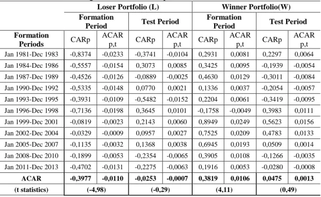
Average monthly cumulative abnormal return is provided at the very bottom of the following table. Accordingly, in the formation period, average monthly cumulative abnormal return of the loser portfolio is 1,1% and it turns out to be -0,07% in the test period. Moreover, average monthly cumulative abnormal return of the winner portfolio becomes 1,06% and it is 0,13% in the test period corresponding to next 36 months period. Accordingly, an investor who buys a loser portfolio loses around -0,07%. On the contrary, an investor who buys a winner portfolio continues to gain 0,13%.
Besides, t statistics value of loser portfolio -0,29 in the test period which is statistically insignificant at the 5% level of significance. Winner portfolio has 0,49 t statistics value in the test period which is also insignificant at the same level. This means there is no significant evidence that shows the reaction of portfolios after formation period.
22
Table 3.1: Abnormal Returns of Winner and Loser Portfolios During 36 months
(Top and bottom 20 firms)
This table presents cumulative abnormal returns and average cumulative abnormal returns at the both 36 months formation and test periods for all portfolios. CAR p is shown as 36 times of ACAR p,t. At the very bottom of the table ACAR is demonstrated which shows the averages of the CAR p and ACAR p,t. At the end of the formation periods, after ranking of cumulative abnormal returns 20 firms are selected at top and bottom. T statistics are calculated to measure significance of ACAR which is the average value of each 11 periods.
Loser Portfolio (L) Winner Portfolio(W)
Formation
Period Test Period
Formation
Period Test Period
Formation Periods CARp ACAR p,t CARp ACAR p,t CARp ACAR p,t CARp ACAR p,t Jan 1981-Dec 1983 -0,8374 -0,0233 -0,3741 -0,0104 0,2931 0,0081 0,2297 0,0064 Jan 1984-Dec 1986 -0,5557 -0,0154 0,3073 0,0085 0,3425 0,0095 -0,1939 -0,0054 Jan 1987-Dec 1989 -0,4526 -0,0126 -0,0889 -0,0025 0,4630 0,0129 -0,3011 -0,0084 Jan 1990-Dec 1992 -0,5335 -0,0148 0,0770 0,0021 0,1336 0,0037 -0,2054 -0,0057 Jan 1993-Dec 1995 -0,3931 -0,0109 -0,5482 -0,0152 0,2204 0,0061 -0,3419 -0,0095 Jan 1996-Dec 1998 -0,7136 -0,0198 0,3645 0,0101 -0,1758 -0,0049 0,3983 0,0111 Jan 1999-Dec 2001 -0,0819 -0,0023 0,2143 0,0060 0,8949 0,0249 0,5623 0,0156 Jan 2002-Dec 2004 -0,0329 -0,0009 0,0957 0,0027 0,7525 0,0209 0,4783 0,0133 Jan 2005-Dec 2007 -0,1135 -0,0032 0,1368 0,0038 0,6945 0,0193 0,0509 0,0014 Jan 2008-Dec 2010 -0,1899 -0,0053 -0,2354 -0,0065 0,3905 0,0108 -0,1266 -0,0035 Jan 2011-Dec 2013 -0,4702 -0,0131 -0,2275 -0,0063 0,1916 0,0053 -0,0280 -0,0008 ACAR -0,3977 -0,0110 -0,0253 -0,0007 0,3819 0,0106 0,0475 0,0013 (t statistics) (-4,98) (-0,29) (4,11) (0,49)
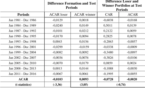
In the left panel of the following table, average monthly cumulative abnormal return is calculated based on the loser and winner stocks and by taking the difference between the formation and test period. If the number of stocks at top and bottom range is 20 in the case of 36 months long formation period, then t-statistics is 3,05 meaning that differences of average returns between portfolio formation and test period is statistically significant. In the case of loser portfolio, as t-statistics is -3,36. In this context, the difference in returns during the formation and test periods is found to be significant in the 95% confidence interval as t-statistics is above the critical t-value.
In addition, these results imply that winner portfolio continue to gain positive abnormal returns and loser portfolio continue to generate negative returns.
23
Far right panel of the following table present a comparison between average abnormal cumulative return of the loser and winner portfolio during the test period. Based on the results provided, one can say that winner portfolio gains 0,2% more than loser portfolio within the test periods considered. T statistics is -0,74 meaning that average return difference between loser and winner portfolio in test period is statistically insignificant because t-statistics is below the critical t-value at 5% significance level.
These result does not confirm the contrarian hypothesis which basically suggests that investor is better-off if she follows a strategy of selling past “winners” and buying past “losers”. Also overreaction hypothesis is not provided with following results because the conditions of hypothesis (ACARW,t<0; ACARL,t>0; (ACARL,t- ACARW,t)>0) are not achieved.
24
Table 3.2: Comparison of ACAR and CAR of Winner and Loser Portfolios During
36 months (Top and bottom 20 firms)
First part of this table presents difference between formation and test periods which is an indicator for contrarian strategy. Second part of table indicates difference between test periods of each winner and loser portfolios. Again ACAR at the bottom shows the averages of each columns.
Difference Formation and Test Periods
Difference Loser and Winner Portfolios at Test
Periods
Periods ACAR loser ACAR winner CAR ACAR
Jan 1981 - Dec 1986 -0,0129 0,0018 -0,6038 -0,0168 Jan 1984 - Dec 1989 -0,0240 0,0149 0,5011 0,0139 Jan 1987 - Dec 1992 -0,0101 0,0212 0,2122 0,0059 Jan 1990 - Dec 1995 -0,0170 0,0094 0,2825 0,0078 Jan 1993 - Dec 1998 0,0043 0,0156 -0,2063 -0,0057 Jan 1996 - Dec 2001 -0,0299 -0,0159 -0,0338 -0,0009 Jan 1999 - Dec 2004 -0,0082 0,0092 -0,3480 -0,0097 Jan 2002 - Dec 2007 -0,0036 0,0076 -0,3826 -0,0106 Jan 2005 - Dec 2010 -0,0070 0,0179 0,0859 0,0024 Jan 2008 - Dec 2013 0,0013 0,0144 -0,1088 -0,0030 Jan 2011 - Dec 2016 -0,0067 0,0061 -0,1995 -0,0055 ACAR -0,0103 0,0093 -0,0728 -0,0020 (t statistics) (-3,36) (3,05) (-0,74)
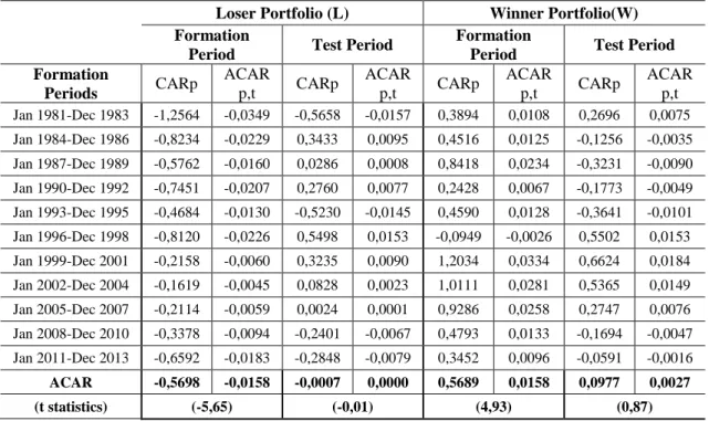
Next table 3.3 presents the results of winner and loser portfolio with top and bottom 10 stocks. So, only difference from the above-given results is the number of stocks at the top-bottom set. To interpret, average cumulative return is -1,58% in the formation period for loser portfolio then it becomes 0,002% in the test period indicating no reverse at all. Average cumulative returns of the winner portfolio are 1,58% and 0,27% in the formation and test period respectively.
Moreover, t statistics value of loser portfolio -0,01 in the test period which is statistically insignificant in the 95% confidence interval. Winner portfolio has 0,87 t statistics value in the test period which is also insignificant at the same level of confidence. This means the reactions of each portfolios after formation period have insignificant t statistics value.
25
Table 3.3: Abnormal Returns of Winner and Loser Portfolios During 36 months
(Top and bottom 10 firms)
This table presents cumulative abnormal returns and average cumulative abnormal returns at the both 36 months formation and test periods for all portfolios. CAR p is shown as 36 times of ACAR p,t. At the very bottom of the table ACAR is demonstrated which shows the averages of the CAR p and ACAR p,t. At the end of the formation periods, after ranking of cumulative abnormal returns 10 firms are selected at top and bottom. T statistics are calculated to measure significance of ACAR which is the average value of each 11 periods.
Loser Portfolio (L) Winner Portfolio(W)
Formation
Period Test Period
Formation
Period Test Period
Formation Periods CARp ACAR p,t CARp ACAR p,t CARp ACAR p,t CARp ACAR p,t Jan 1981-Dec 1983 -1,2564 -0,0349 -0,5658 -0,0157 0,3894 0,0108 0,2696 0,0075 Jan 1984-Dec 1986 -0,8234 -0,0229 0,3433 0,0095 0,4516 0,0125 -0,1256 -0,0035 Jan 1987-Dec 1989 -0,5762 -0,0160 0,0286 0,0008 0,8418 0,0234 -0,3231 -0,0090 Jan 1990-Dec 1992 -0,7451 -0,0207 0,2760 0,0077 0,2428 0,0067 -0,1773 -0,0049 Jan 1993-Dec 1995 -0,4684 -0,0130 -0,5230 -0,0145 0,4590 0,0128 -0,3641 -0,0101 Jan 1996-Dec 1998 -0,8120 -0,0226 0,5498 0,0153 -0,0949 -0,0026 0,5502 0,0153 Jan 1999-Dec 2001 -0,2158 -0,0060 0,3235 0,0090 1,2034 0,0334 0,6624 0,0184 Jan 2002-Dec 2004 -0,1619 -0,0045 0,0828 0,0023 1,0111 0,0281 0,5365 0,0149 Jan 2005-Dec 2007 -0,2114 -0,0059 0,0024 0,0001 0,9286 0,0258 0,2747 0,0076 Jan 2008-Dec 2010 -0,3378 -0,0094 -0,2401 -0,0067 0,4793 0,0133 -0,1694 -0,0047 Jan 2011-Dec 2013 -0,6592 -0,0183 -0,2848 -0,0079 0,3452 0,0096 -0,0591 -0,0016 ACAR -0,5698 -0,0158 -0,0007 0,0000 0,5689 0,0158 0,0977 0,0027 (t statistics) (-5,65) (-0,01) (4,93) (0,87)
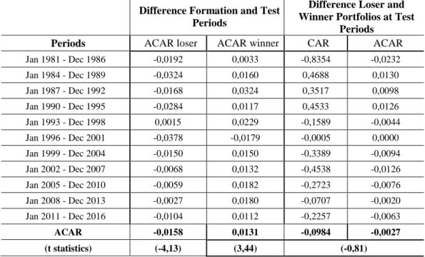
If the number of stocks at top and bottom range is 10 in the case of 36 months long formation period, then t-statistics is 3,44 indicating statistically significant difference between portfolio formation and test period. Likewise, loser portfolio, with a t-statistics of -4,13 suggests the same result. Thus, the difference in returns during the formation and test periods is found to be significant in the 95% confidence interval as t-statistics is above the critical t-value.
Additionally, winner portfolio generates 0,27% more return than loser portfolio during the test period. This result indicates that shrinking the number of loser and winner stocks at the top and bottom series does not change the result in
26
this case. T statistics is -0,81 indicating statistically insignificant difference between loser and winner portfolio in test period again.
Table 3.4: Comparison of ACAR and CAR of Winner and Loser Portfolios During
36 months (Top and bottom 10 firms)
First part of this table presents difference between formation and test periods which is an indicator for contrarian strategy. Second part of table indicates difference between test periods of each winner and loser portfolios. Again ACAR at the bottom shows the averages of each columns.
Difference Formation and Test Periods
Difference Loser and Winner Portfolios at Test
Periods
Periods ACAR loser ACAR winner CAR ACAR
Jan 1981 - Dec 1986 -0,0192 0,0033 -0,8354 -0,0232 Jan 1984 - Dec 1989 -0,0324 0,0160 0,4688 0,0130 Jan 1987 - Dec 1992 -0,0168 0,0324 0,3517 0,0098 Jan 1990 - Dec 1995 -0,0284 0,0117 0,4533 0,0126 Jan 1993 - Dec 1998 0,0015 0,0229 -0,1589 -0,0044 Jan 1996 - Dec 2001 -0,0378 -0,0179 -0,0005 0,0000 Jan 1999 - Dec 2004 -0,0150 0,0150 -0,3389 -0,0094 Jan 2002 - Dec 2007 -0,0068 0,0132 -0,4538 -0,0126 Jan 2005 - Dec 2010 -0,0059 0,0182 -0,2723 -0,0076 Jan 2008 - Dec 2013 -0,0027 0,0180 -0,0707 -0,0020 Jan 2011 - Dec 2016 -0,0104 0,0112 -0,2257 -0,0063 ACAR -0,0158 0,0131 -0,0984 -0,0027 (t statistics) (-4,13) (3,44) (-0,81)
Following analysis presents a result with 5 winner/loser stocks at top and bottom range. Accordingly, loser portfolio in the formation period generates -2,02% while, in the test period, loser portfolio’s monthly return turns out to be positive (0,13%). Winner portfolio, however, has positive return both in formation and test period. In the formation period 5 winner stock generate a return of 2,12% and 0,23% in the test period. This case is different compared to other to two cases in that loser portfolio’s return turned from negative to positive.
Besides that, t statistics value of loser portfolio 0,36 in the test period which is statistically insignificant in the 95% confidence interval. Winner portfolio has 0,79 t statistics value in the test period which is also insignificant at the same level of confidence interval. This means reaction of portfolios after formation period does
27
not reflect any significant evidence at the 5% significance level.
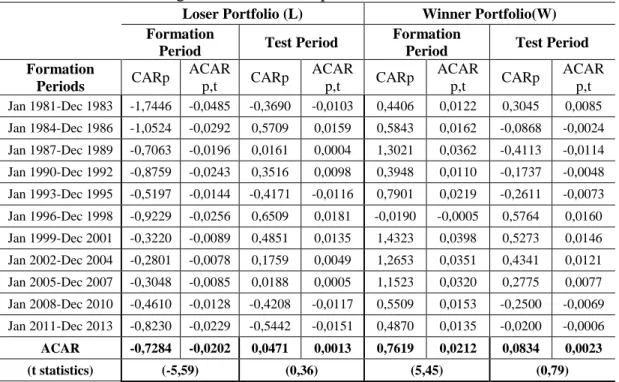
Table 3.5: Abnormal Returns of Winner and Loser Portfolios During 36 months
(Top and bottom 5 firms)
This table presents cumulative abnormal returns and average cumulative abnormal returns at the both 36 months formation and test periods for all portfolios. CAR p is shown as 36 times of ACAR p,t. At the very bottom of the table ACAR is demonstrated which shows the averages of the CAR p and ACAR p,t. At the end of the formation periods, after ranking of cumulative abnormal returns 5 firms are selected at top and bottom. T statistics are calculated to measure significance of ACAR which is the average value of each 11 periods.
Loser Portfolio (L) Winner Portfolio(W)
Formation
Period Test Period
Formation
Period Test Period
Formation Periods CARp ACAR p,t CARp ACAR p,t CARp ACAR p,t CARp ACAR p,t Jan 1981-Dec 1983 -1,7446 -0,0485 -0,3690 -0,0103 0,4406 0,0122 0,3045 0,0085 Jan 1984-Dec 1986 -1,0524 -0,0292 0,5709 0,0159 0,5843 0,0162 -0,0868 -0,0024 Jan 1987-Dec 1989 -0,7063 -0,0196 0,0161 0,0004 1,3021 0,0362 -0,4113 -0,0114 Jan 1990-Dec 1992 -0,8759 -0,0243 0,3516 0,0098 0,3948 0,0110 -0,1737 -0,0048 Jan 1993-Dec 1995 -0,5197 -0,0144 -0,4171 -0,0116 0,7901 0,0219 -0,2611 -0,0073 Jan 1996-Dec 1998 -0,9229 -0,0256 0,6509 0,0181 -0,0190 -0,0005 0,5764 0,0160 Jan 1999-Dec 2001 -0,3220 -0,0089 0,4851 0,0135 1,4323 0,0398 0,5273 0,0146 Jan 2002-Dec 2004 -0,2801 -0,0078 0,1759 0,0049 1,2653 0,0351 0,4341 0,0121 Jan 2005-Dec 2007 -0,3048 -0,0085 0,0188 0,0005 1,1523 0,0320 0,2775 0,0077 Jan 2008-Dec 2010 -0,4610 -0,0128 -0,4208 -0,0117 0,5509 0,0153 -0,2500 -0,0069 Jan 2011-Dec 2013 -0,8230 -0,0229 -0,5442 -0,0151 0,4870 0,0135 -0,0200 -0,0006 ACAR -0,7284 -0,0202 0,0471 0,0013 0,7619 0,0212 0,0834 0,0023 (t statistics) (-5,59) (0,36) (5,45) (0,79)
If the number of stocks at top and bottom range is 5 in the case of 36 months long formation period, then t-statistics is 3,92 meaning that average return differences between portfolio formation and test period is statistically significant. Similarly, loser portfolio has a t-value of -4,37 which amounts to statistically significant difference between mean return in formation and test period.
An investor who buys loser portfolio gains 0,13% but an investor who buys winner portfolio gains 0,23% average monthly cumulative abnormal returns. Finally, winner portfolio generate 0,10% returns more than the loser portfolio which contradicts with the contrarian hypothesis. Statistically insignificant
28
difference between loser and winner portfolios in test period again based on t statistics is -0,28. The results verify that there is no significant evidence that shows overreaction.
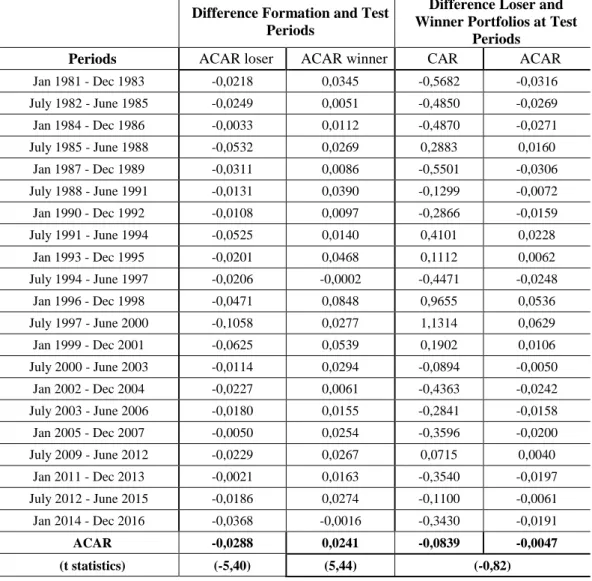
Table 3.6: Comparison of ACAR and CAR of Winner and Loser Portfolios During
36 months (Top and bottom 5 firms)
First part of this table presents difference between formation and test periods which is an indicator for contrarian strategy. Second part of table indicates difference between test periods of each winner and loser portfolios. Again ACAR at the bottom shows the averages of each columns.
Difference Formation and Test Periods
Difference Loser and Winner Portfolios at Test
Periods
Periods ACAR loser ACAR winner CAR ACAR
Jan 1981 - Dec 1986 -0,0382 0,0038 -0,6736 -0,0187 Jan 1984 - Dec 1989 -0,0451 0,0186 0,6576 0,0183 Jan 1987 - Dec 1992 -0,0201 0,0476 0,4274 0,0119 Jan 1990 - Dec 1995 -0,0341 0,0158 0,5253 0,0146 Jan 1993 - Dec 1998 -0,0028 0,0292 -0,1560 -0,0043 Jan 1996 - Dec 2001 -0,0437 -0,0165 0,0745 0,0021 Jan 1999 - Dec 2004 -0,0224 0,0251 -0,0422 -0,0012 Jan 2002 - Dec 2007 -0,0127 0,0231 -0,2582 -0,0072 Jan 2005 - Dec 2010 -0,0090 0,0243 -0,2587 -0,0072 Jan 2008 - Dec 2013 -0,0011 0,0222 -0,1708 -0,0047 Jan 2011 - Dec 2016 -0,0077 0,0141 -0,5243 -0,0146 ACAR -0,0215 0,0188 -0,0363 -0,0010 (t statistics) (-4,37) (3,92) (-0,28)
3.3.1. Excluding Crisis Period
One of the major contribution of this study is to control for the effect of the global mortgage crisis hit hard and deep the most of the economies across the world. In the first part of the analysis, the crisis period is included and but in this part two different analyzes are conducted so that the effect of the crisis on the winner/loser portfolios can be properly addressed.
To do that, I refer the National Bureau of Economic Research (NBER) to identify the peak and trough periods of the mortgage crisis. As is known, U.S recessions are arranged in chronological order by NBER according to beginning
29
and ending dates. The NBER’s Business Cycle Dating Committee defines a recession as “a significant decline in economic activity spread across the economy, lasting more than a few months, normally visible in production, employment, real income, and other indicators. A recession begins when the economy reaches a peak of activity and ends when the economy reaches its trough.” Consistent with this definition, the Committee focuses on a universal set of evaluates including not only GDP, but also employment, income, sales, and industrial production to investigate the trends in economic activity1.
Within this context, NBER’s peak and trough periods are Dec 2007-June 2009, respectively. To be consistent with these dates, time period of this specific analysis is 18 months meaning that there is 18 months period between Dec 2007-June 2009, the rest of the period starting on Jan 1981 and ending on Dec 2016 is divided into 21x18 months period. By doing that 18 months crisis periods are excluded. In the case at which crisis is neglected, whole time period is divided into 23x18 months period. By doing that, I have the opportunity to properly observe the effect of the crisis on the overreaction hypothesis.
Firstly, the effect of the crisis is not taken separately and prior and post 18 months are the periods in this part. In this analysis, only the results of returns 5 top and bottom range portfolios are presented because of higher t statistics value. Other results for top and bottom 10 and 20 firms are presented in appendix part. Accordingly, loser portfolio in the formation period generates -2,81% while, in the test period, loser portfolio’s monthly return same negative as -0,01%. Winner portfolio, however, has positive return both in formation and test period. Likewise the sign of the returns of both loser and winner are not changed from formation to test period.
Following table also presents the t-statistics of loser and winner portfolios between formation and test period so that one can conclude whether return
30
difference is statistically significant between formation and test period. T statistics value of loser portfolio -0,02 and winner portfolio has 1,12 t statistics value in the test periods which are also insignificant at the same level of confidence. This means reaction of portfolios after formation period does not reflect any significant evidence at the 5% significance level.
31
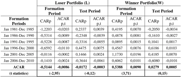
Table 3.7: Abnormal Returns of Winner and Loser Portfolios During 18 months
(Top and bottom 5 firms)
This table presents cumulative abnormal returns and average cumulative abnormal returns at the both 18 months formation and test periods for all portfolios. CAR p is shown as 18 times of ACAR p,t. At the very bottom of the table ACAR is demonstrated which shows the averages of the CAR p and ACAR p,t. At the end of the formation periods, after ranking of cumulative abnormal returns 5 firms are selected at top and bottom. T statistics are calculated to measure significance of ACAR which is the average value of each 23 periods.
Loser Portfolio (L) Winner Portfolio(W)
Formation
Period Test Period
Formation
Period Test Period
Formation Periods CARp ACAR p,t CARp ACAR p,t CARp ACAR p,t CARp ACAR p,t Jan 1981-June 1982 -1,0683 -0,0593 -0,6763 -0,0376 0,5137 0,0285 -0,1081 -0,0060 July 1982-Dec 1983 -0,7827 -0,0435 -0,3341 -0,0186 0,2427 0,0135 0,1509 0,0084 Jan 1984-June 1985 -0,4518 -0,0251 -0,3931 -0,0218 0,2957 0,0164 0,0939 0,0052 July 1985-Dec 1986 -0,6828 -0,0379 0,2748 0,0153 0,4698 0,0261 -0,0135 -0,0008 Jan 1987-June 1988 -0,5362 -0,0298 0,0240 0,0013 0,7280 0,0404 0,5741 0,0319 July 1988-Dec 1989 -0,4044 -0,0225 -0,1688 -0,0094 0,6630 0,0368 -0,0390 -0,0022 Jan 1990-June 1991 -0,4450 -0,0247 -0,2503 -0,0139 0,2103 0,0117 0,0363 0,0020 July 1991-Dec 1992 -0,5169 -0,0287 0,4287 0,0238 0,2701 0,0150 0,0186 0,0010 Jan 1993-June 1994 -0,3860 -0,0214 -0,0239 -0,0013 0,7071 0,0393 -0,1351 -0,0075 July 1994-Dec 1995 -0,5658 -0,0314 -0,1950 -0,0108 0,2492 0,0138 0,2522 0,0140 Jan 1996-June 1997 -0,7237 -0,0402 0,1241 0,0069 0,6845 0,0380 -0,8414 -0,0467 July 1997-Dec 1998 -1,0216 -0,0568 0,8825 0,0490 0,2491 0,0138 -0,2490 -0,0138 Jan 1999-June 2000 -0,7046 -0,0391 0,4209 0,0234 1,2016 0,0668 0,2307 0,0128 July 2000-Dec 2001 0,0406 0,0023 0,2455 0,0136 0,8643 0,0480 0,3349 0,0186 Jan 2002-June 2003 -0,3277 -0,0182 0,0817 0,0045 0,6274 0,0349 0,5180 0,0288 July 2003-Dec 2004 -0,1867 -0,0104 0,1370 0,0076 0,7007 0,0389 0,4211 0,0234 Jan 2005-June 2006 -0,1206 -0,0067 -0,0301 -0,0017 0,7868 0,0437 0,3295 0,0183 July 2006-Dec 2007 -0,3111 -0,0173 0,1534 0,0085 0,4759 0,0264 0,2688 0,0149 Jan 2008-June 2009 -0,2195 -0,0122 0,0406 0,0023 0,5572 0,0310 -0,1733 -0,0096 July 2009-Dec 2010 -0,4613 -0,0256 -0,0500 -0,0028 0,3583 0,0199 -0,1214 -0,0067 Jan 2011-June 2012 -0,3699 -0,0206 -0,3325 -0,0185 0,3142 0,0175 0,0215 0,0012 July 2012-Dec 2013 -0,6308 -0,0350 -0,2968 -0,0165 0,3061 0,0170 -0,1868 -0,0104 Jan 2014-June 2015 -0,7494 -0,0416 -0,0874 -0,0049 0,2267 0,0126 0,2556 0,0142 ACAR -0,5055 -0,0281 -0,0011 -0,0001 0,5088 0,0283 0,0712 0,0040 (t statistics) (-8,96) (-0,02) (9,47) (1,12)
It can be readily observable that all the t-values between formation and test periods are larger than the critical value. It is, therefore, concluded that return