Explicit Exponential Finite Difference Methods for the Numerical Solution of Modified Burgers’ Equation

ISSN: 2149-6137

Explicit Exponential Finite Difference Methods for the Numerical Solution of Modified

Burgers’ Equation

GONCA ÇELİKTEN1

and EMİNE NESLİGÜL AKSAN2

1 _{Kafkas University, Faculty of Science and Letters, Department of Mathematics, 36100, Kars, Turkey.}

2 _{Inönü University, Faculty of Science and Letters, Department of Mathematics, 44280, Malatya, Turkey.}

Abstract

In this study, explicit exponential finite difference schemes based on four different linearization techniques are given for the numerical solutions of the Modified Burgers' equation. A model problem is used to verify the efficiency and accuracy of the methods that we proposed. Also comparisons are made with the relevant ones in the literature. It is shown that all results that are found to be in good agreement with those available in the literature.

2

L and L_ error norms are calculated. The obtained error norms are suciently small in all computer runs. The results show that the present method is a successful numerical scheme for solving the Modified Burgers' equation.

Keywords: Burgers’ equation, Modified Burgers’ equation,

Explicit exponential finite difference method Introduction

Burgers’ equation was first given by Bateman (BATEMAN (1915)) and later was studied by Burgers (BURGERS (1939), BURGERS (1948)) as a mathematical model for turbulence. Since it has an extensive usage in engineering and other scientific fields, the Burgers’ equation has found applications in various fields such as convection and diffusion, number theory, gas dynamics, heat conduction, elasticity etc (ROSHAN and BHAMRA (2011)). The one-dimensional generalized Burgers’ equation is in the form

0 , 1, 2

p

t x xx

u u u vu  a x b p

in which

u

denotes the velocity for space

x

and time t and

v



0

is a constant representing the knematics viscosity of the fluid. It is known as Burgers’ equation and modified Burgers’ equation for p1 and p2, respectively.

Received: 10.09.2016 Revised: 10.12.2016 Accepted:15.12.2016

Corresponding author: Gonca Çelikten

Kafkas University, Faculty of Science and Letters, Department of Mathematics, 36100, Kars, Turkey

E-mail: gnc.cnbk@gmail.com

Cite this article as: G. Çelikten and E.N. Aksan, Explicit Exponential Finite Difference Methods for the Numerical Solution of Modified Burgers’ Equation, Eastern Anatolian Journal of Science, Vol. 3, Issue 1, 45-50, 2017.

Many analytical and numerical solutions of equation have been published by a number of authors using different methods and techniques. An analytical solution of Burgers’ equation was given by Benton and Platzman (BENTON and PLATZMAN (1972)). Infinite series solutions of the equation have been introduced by Miller (MILLER (1966)) Kutluay et al. (KUTLUAY et al. (1999)) have obtained numerical solutions of one-dimensional Burgers’ equations by using explicit and exact-explicit finite difference methods. A finite element approach was used to obtain the numerical solution of Burgers’ equations by Öziş et al. (ÖZİŞ et al. (2003)). Dag et al. (DAG et al. (2005)) have obtained numerical solutions of the Burgers’ equations by using B-spline collocation methods. Variational iteration method has been used to solve Burgers and coupled Burgers equations by Abdou and Soliman (ABDOU and SOLIMAN (2005)). The problem we deal with is in general form:

2

0

t x xx

u u u vu  a x b,

t



t

₀

with initial condition



x

t



f

 

x

u

,

0



and boundary conditions

 

a

t

g

 

t

u

,



₁ ,

u

 

b

,

t



g

₂

 

t

where x and t are independent variables, uu x t( , ),

 

a,

b

is the solution region



a

,

b



R



, v is the viscosity parameter,

f

 

x

,

g

₁

 

t

and

g

₂

 

t

are known functions.

In the present work, main aim is to apply the explicit exponential finite difference methods to improve a numerical method for the modified Burgers’ equation. In the literature many numerical method was applied to approximate the solution of the modified Burgers equation by several authors. Ramadan and El-Danaf (RAMADAN and EL-DANAF (2005)) used the collocation method with quintic splines for the solution of equation. Then, the equation has been solved by Ramadan et al. (RAMADAN et al. (2005)) using the colocation method with septic splines. Burgers and the

modified burgers equations are solved numerically by using the time and space splitting techniques to equations, and then using B-spline collocation procedure to approximate the resulting systems by Saka and Dag (SAKA and DAG (2008)). Numerical solutions of modified Burgers’ equation was obtained by using sextic B-spline collocation method by Irk (IRK (2009)). Grienwank and El-Danaf (GRIENWANK and EL-DANAF (2009)) obtained the numerical solutions of the modified Burgers’ equation by using a non-polynomial spline based method. Bratsos and Petrakis (BRATSOS and PETRAKIS (2011)) used an explicit numerical scheme for solving the modified Burgers’ equation. The equation has been numerically solved by Roshan and Bhamra (ROSHAN and BHAMRA (2011)) by the Petrov-Galerkin Method.

The explict exponential finite difference method have been improved by Bhattacharya (BHATTACHARYA (1985)) for the solution of heat equation. Bhattacharya (BHATTACHARYA (1990)) and Handschuh-Keith (HANDSCHUH and KEITH (1992)) used the exponential finite difference technique to obtain numerical solutions of Burgers’ equation. Bahadır (BAHADIR (2005)) obtained the numerical solutions of KdV equation for small times by applying the exponential finite difference method. Implicit exponential finite difference method and fully implicit exponential finite difference method were used to solve the Burgers’ equation by Inan and Bahadır (INAN and BAHADIR (2013)) The Burgers’ equation has been numerically solved by Inan and Bahadır (INAN and BAHADIR (2013)) by applying the Hopf-Cole transformation to equation and then employed the explicit exponential finite difference method to approximate the resulting heat equation.

Model Problem and Numerical Method Model Problem

We consider the initial boundary value problem for modified Burgers’ equation

u

_t



u

2

u

_x



vu

_xx

,

0



x



1

,

t



1

(1) with initial condition

 





v

x

c

x

x

u

4

/

exp

)

/

1

(

1

1

,

₂ 0





(2)

and boundary conditions

 

0

,

t



0

u

,

 







vt



c

t

t

t

u

4

/

1

exp

/

1

/

1

,

1

0





. (3)

Following (HARRIS (1996)) modified Burgers’ equation (1) has the analytic solution

 

_

_

vt

x

c

t

t

x

t

x

u

4

/

exp

)

/

(

1

/

,

2 0





where c is a constant, ₀ 0c₀ 1. Numerical Method

To obtain numerical solutions, the solution region of the problem

0



x



1

is divided by N equal subintervals of length h. We indicate the finite difference approximation of

u

( t

x

,

)

at the mesh point

(

x

_i

,

t

_n

)

by

u

_in in which

ih

x

_i



(

i



0

,

1

,



,

N

)

,

t

_n



t

₀



nk

)

,

2

,

1

,

0

(

n





,

N

h



1



0

is the mesh size in

x

direction and

k

is the time step.

Now let us express the finite difference schemes of the initial condition (2) and the boundary condition (3), respectively, 

_

_

v

x

c

x

u

i i i

4

/

exp

)

/

1

(

1

1

/

2 0 0





and 

u

₀n



0

, 



n



n n n N

vt

c

t

t

u

4

/

1

exp

)

/

(

1

/

1

0





.

We follow the procedure of ref. (BAHADIR (2005)) to examine the numerical method. If we suppose that F u

 

is any continuous differential function and multiplying equation (1) by F

u



 the following equation is obtained:

 

2 2 2 F u u u F u u v u t x x            













and

 

2 2 2 . F u u F u u v t x x          













(4)

Using the forward difference approximation for F t

  the

finite difference representation of equation (4) is obtained as:

   

 

2 1 2 2 n n n n n i i i i i u u F u F u kF u u v x x  _{   }  _   



_

_

_

_





_

_

_

_



















in which k is the time step. Let F u

 

lnu then the expilicit exponential finite difference scheme for equation (1) is obtained as: 2 1 2 2 exp n n n n i i n i i i k u u u u u v u x x  _{ }  _   





_

_







_





_







_



_

















_

_







(5)

If we use central difference approximation in place of 2 2 u x   in equation (5) 2 1 1 2 2 2 , 1 i N-1 n _{n n n} i i i i u u u u x h         













and then apply the following linearization techniques in place of the non-linear term u2 u

x  

 

2 2 1 1 2 2 1 1 1 FD-I. , 1 i N-1 2 FD-II. , 1 i N-1 2 2 n n n n i i i i n n n n n i i i i i u u u u u x h u u u u u u x h     _{   }         _{ }       _{      }     _  _{ } _   _{   }   _{  }     _{  }  2 2 1 1 1 FD-III. , 1 i N-1 2 2 n n n n n i i i i i u u u u u u x h       _{      }     _{   }   _{   }    _{  }  2 2 1 1 1 1 FD-IV. , 1 i N-1 3 2 n n n n n n i i i i i i u u u u u u u x h       _{       }           _{   }     _{  } 

respectively, we obtained the following explicit exponential finite difference schemes



 



1 E-EFDM-I. exp _{1 1 1} 2 ₁ 2 n n k n n n rv n n n u_i u_i u_i u_i u_i u_i u_i u_i n h _u i          _ _  _  _    



_{ }

_{ }

_

E-EFDM-II. 2 1 1 exp _{1 1 1} 2 ₁ , 8 n n u u n n k i i n n rv n n n u_i u_i u_i u_i u_i u_i u_i n n h _{u u} i i       _ _  _{   } _          



_{ }

2

_{ }

_

1 1 E-EFDM-III. exp _{1 1 1} 2 ₁ , 8 n n u_i u_i k rv n n n n n n n u_i u_i u_i u_i u_i u_i u_i n n h _{u u} i i     _       _  _  _  _       



_{ }

_{ }

_

E-EFDM-IV. 2 1 1 1 exp _{1 1 1} 2 ₁ , 18 n n n u u u n n k i i i n n rv n n n u_i u_i u_i u_i u_i u_i u_i n n h _{u u} i i        _ _   _{   } _           respectively, where r k₂, 1 i N-1 h    .

Numerical Results and Discussion

Numerical solutions of model problem are obtained by explicit exponential finite difference method. To show the accuracy of the results, L₂ and L_error norms:

 

2 2 ₂ 0 N N j N _j j L u U h u U       ,

 

max N _j j N j L_  uU _  u  U

are used, in which

u

and

U

_N represent analytic and computed numerical solutions respectively. Numerical solutions are obtained at different times for different values of v, h,



t

and c₀ 0.5. The obtained results are displayed in Table 1-6 and Figure 1-2. Table 1 and Table 2 present L₂ and L_error norms with

v



0.001

,

0.0125

h ,

 

t

0.01

at different times. L₂ and L_ error norms of explicit exponential finite difference schemes at t_f 2 for

v



0.01

and

 

t

0.001

for different values of h are given in Table 3 and Table 4, respectively. It is seem that the values of L₂ and L_ decrease with decrease of h in Table 3 and Table 4, respectively. The obtained error norms L₂ and L_of present study are compared with other methods (RAMADAN and EL-DANAF (2005), IRK (2009)) for

0.005

v



,h0.005 and

 

t

0.001

at times 2, 6,10

t in Table 5. The obtained error norms L₂ and L_ of the present study are compared with other methods (RAMADAN et. al. (2005), SAKA and DAG (2008), IRK (2009)) for

v



0.01

, h0.02 and

 

t

0.01

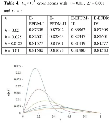
at times t2, 6,10 in Table 6. As seen from the Tables 5-6, it is observed that the obtained results using the explicit exponential finite difference schemes are in good agreement with those available in the literature. Figures 1 and 2 show behavior of the numerical solutions for

0.01

v



and

v



0.005

with h0.05,

 

t

0.01

at times t 1, 2, 4, 6, 8,10 for E-EFDM-I. The top and bottom curves are at t1 and t 10, respectively. It can be seen from the figures that the curve of the numerical solution decays as the time increases. Note that as the viscosity parameter v gets small the decay gets fast.

Table 1. L₂103 error norms with v0.001, h0.0125 and  t 0.01. t E-EFDM-I E-EFDM-II E-EFDM-III E-EFDM-IV 2 0.070907 0.070925 0.070888 0.070916 3 0.061455 0.061509 0.061394 0.061455 4 0.054713 0.054778 0.054640 0.054710 5 0.050197 0.050263 0.050122 0.050193 6 0.046844 0.046908 0.046772 0.046840 7 0.044160 0.044220 0.044092 0.044156 8 0.041909 0.041966 0.041845 0.041905 9 0.039966 0.040020 0.039906 0.039963 10 0.038257 0.038307 0.038200 0.038254

Table 2. L_103 error norm with v0.001, h0.0125 and  t 0.01. t E-EFDM-I E-EFDM-II E-EFDM-III E-EFDM-IV 2 0.257336 0.257714 0.256925 0.257335 3 0.223175 0.223464 0.222852 0.223164 4 0.186933 0.187179 0.186657 0.186920 5 0.160985 0.161194 0.160751 0.160973 6 0.141988 0.142166 0.141787 0.141977 7 0.127328 0.127483 0.127154 0.127319 8 0.115506 0.115642 0.115353 0.115497 9 0.105649 0.105769 0.105513 0.105641 10 0.097656 0.097771 0.097526 0.097648 Table 3. L₂103 error norms with v0.01,  t 0.001 and t_f 2. h E- EFDM-I E- EFDM-II E- EFDM-III E- EFDM-IV 0.05 h 0.43128 0.43130 0.43074 0.43128 0.025 h 0.39014 0.39040 0.38975 0.39014 0.0125 h 0.38071 0.38088 0.38051 0.38071 0.01 h 0.37961 0.37975 0.37944 0.37961

Table 4. L_103 error norms with v0.01,  t 0.001 and t_f 2. h E-EFDM-I E-EFDM-II E-EFDM-III E-EFDM-IV 0.05 h 0.87308 0.87702 0.86863 0.87308 0.025 h 0.82601 0.82843 0.82347 0.82601 0.0125 h 0.81577 0.81701 0.81449 0.81577 0.01 h 0.81580 0.81678 0.81480 0.81580

Figure 1. Numerical solutions for v0.01 with h0.05 ,  t 0.01 at times t1, 2, 4, 6, 8,10 for E-EFDM-I.

Figure 2. Numerical solutions for v0.005with Conclusions

In this study, explicit exponential finite difference schemes based on four different linearization techniques have been proposed for the numerical solutions of the Modified Burgers' equation. A model problem is used to verify the efficiency and accuracy of the schemes that we proposed. Also comparisons were made with the relevant ones in the literature. L₂ and L_ error norms have been calculated and given. The obtained error norms are sufficiently small in all computer runs. The results show that this method is a successful numerical scheme for solving the modified Burgers' equation. h0.05,

0.01 t

Table 5. Comparison of the error norms L₂ and L_with those in other studies in the literature at t2, 6,10 for 0.005 h ,  t 0.001 and v0.005.

2

t



t



6

t



10

3 2 10 L  L_103 L₂103 L_103 L₂103 L_103

E-EFDM-I

0.22610 0.57843 0.16368 0.32834 0.13882 0.22770

E-EFDM-II

0.22615 0.57877 0.16377 0.32851 0.13890 0.22782

E-EFDM-III

0.22605 0.57808 0.16358 0.32816 0.13875 0.22759

E-EFDM-IV

0.22610 0.57843 0.16368 0.32833 0.13882 0.22770

(RAMADAN AND EL-DANAF (2005)) 0.25786 0.72264 0.22569 0.43082 0.18735 0.30006

(IRK (2009)) (SBCM1) 0.22890 0.58623 - - 0.14042 0.23019

(IRK (2009)) (SBCM2) 0.23397 0.58424 - - 0.13747 0.22626

Table 6. Comparison of the error norms L₂ and L_with those in other studies in the literature at t2, 6,10 for h0.02, 0.01 t   and v0.01.

2

t



t



6

t



10

3 2 10 L  L_103 L₂103 L_103 L₂103 L_103

E-EFDM-I

0.37027 0.78740 0.31581 0.52579 0.55159 1.28125

E-EFDM-II

0.37053 0.78941 0.31636 0.52579 0.55187 1.28125

E-EFDM-III

0.37000 0.78531 0.31524 0.52579 0.55129 1.28125

E-EFDM-IV

0.37031 0.78740 0.31580 0.52579 0.55158 1.28125

(RAMADAN ET. AL. (2005)) 0.79043 1.70309 0.51672 0.76105 0.80026 1.80239

(SAKA AND DAG (2008)) (QBCA1) 0.37911 0.81254 0.32941 0.52579 0.55848 1.28125 (SAKA AND DAG (2008)) (QBCA2) 0.39473 0.88383 0.31588 0.53910 0.52425 1.28125

(IRK (2009)) (SBCM1) 0.38474 0.82611 - - 0.55985 1.28127

(IRK (2009)) (SBCM2) 0.41321 0.81502 - - 0.55095 1.28127

References

ABDOU, M. A., SOLIMAN, A. A. (2005) Variational iteration method for solving Burger’ s and coupled Burger’ s equations, Journal of Computational and Applied Mathematics 181, 245-251.

BAHADIR, A. R. (2005) Exponential finite-difference method applied to Korteweg-de Vries equation for small times, Applied Mathematics and Computation 160, 675-682.

BATEMAN, H. (1915) Some recent reseaches on the motion of fluids,Samantaray, Mon. Weather Rev. 43, 163-170.

BENTON, E. L., PLATZMAN, G. W. (1972) A table of solutions of the one-dimensional Burgers equations, Quart. Appl. Math. 30, 195-212. BHATTACHARYA, M. C. (1985) An explicit

conditionally stable finite difference equation for heat conduction problems, International Journal for Numerical Methods in Engineering, 21, 239-265.

BHATTACHARYA, M. C. (1990) Finite Difference Solutions of Partial Differential Equations, Communications in Applied Numerical Methods, 6, 173-184.

BRATSOS, A. G., PETRAKİS, L. A. (2011) An explicit numerical scheme for the modified Burgers' equation, International Journal for Numerical Methods in Biomedical Engneering, 27:232-237. BURGERS, J. M. (1939) Mathematical examples illustrating relations occuring in the theory of turbulent fluid motion, Trans. R. Neth. Acad. Sci. Amst. 17, 1-53.

BURGERS, J. M. (1948) A mathematical model illustrating the theory of turbulence, Adv. Appl. Mech. 1, 171-199.

DAG, I., IRK, D., SAHIN, A. (2005) B-spline collocation methods for numerical solutions of the Burgers equation, Mathematical Problems in Engineering 2005:5, 521-538.

GRIEWANK, A., EL-DANAF, T. S. (2009) Efficient accurate numerical treatment of the modified

Burgers' equation, Applicable Analysis, vol. 88, No. 1, 75-87.

HANDSCHUH, R. F., KEITH, T. G. (1992) Applications of an exponential finite-difference technique, Numerical Heat Transfer, 22, 363-378.

HARRIS, S. E. (1996) Sonic shocks governed by the modified Burgers' equation, Eur. J. Appl. Math. 7 (2) , 201_222.

INAN, B., BAHADIR, A. R. (2013) An explicit exponential finite difference method for the Burgers’ equation, European International Journal of Science and Technology Vol. 2 No. 10, pp. 61-72.

INAN, B., BAHADIR, A. R. (2013) Numerical solution of the one-dimensional Burgers’ equation: Implicit and fully implicit exponential finite difference methods, Pramana – J. Phys., Vol. 81,

No. 4, pp. 547-556.

IRK, D. (2009) Sextic B-spline collocation method for the modified Burgers' equation, Kybernetes, Vol. 38, No. 9, pp. 1599-1620.

KUTLUAY, S., BAHADIR, A. R., OZDES, A. (1999) Numerical solution of one-dimensional Burgers equation: explicit and exact-explicit finite difference methods, Journal of Computational and Applied Mathematics 103, 251-261.

MILLER, E. L. (1966) Predictor-Corrector studies of Burger's model of turbulnet flow, M.S. Thesis, University of Delaware, Newark, Delaware. ÖZIS, T., AKSAN, E. N., OZDES, A. (2003) A finite

element approach for solution of Burgers’ equation, Applied Mathematics and Computation 139, 417-428.

RAMADAN, M. A., EL-DANAF, T. S. (2005) Numerical treatment for the modified Burgers equation, Matmematics and Computers in Simulation 70, 90-98.

RAMADAN, M. A., EL-DANAF, T. S., ABD ALAAL, F. E. I. (2005) A numerical solution of the Burgers equation using septic B-splines, Chaos, Solitons and Fractals 26, 795-804.

ROSHAN, T., BHAMRA, K. S. (2011) Numerical solutions of the modified Burgers' equation by Petrov-Galerkin method, Applied Mathematics and Computation, 218, 3673-3679.

SAKA, B., DAG, I. (2007) Quartic B-spline collocation methods to the numerical solutions of the Burgers' equation, Chaos, Solitons & Fractals 32, 1125-1137.

SAKA, B., DAG, I. (2008) A numerical study of the Burgers' equation, Journal of the Franklin Institute 345, 328-348.