Using WEPP Model to Predict Sediment and Runoff from
an Agricultural Watershed
Halil KIRNAK1 Prasanna H. GOWDA2
Geliş Tarihi : 02.01.2001
Abstract: The WEPP (VVater Erosion Prediction Project) model was used in conjunction with a GIS database to predict flow and sediment discharges for Rock Creek watershed-an agricultural watershed in Ohio, USA. Spatial data layers of slope, soil type, land use and tillage practices were combined with a Geographic Information System (GIS). Observed and predicted mean monthly values were compared from 1988 to 1990. The WEPP model was applied to Rock Creek watershed both by complying with size limitation of the model (less than 260 ha) and not. In case of not keeping watershed size limit, statistical results showed that model simulation for sediment and runoff were poor with an r2 of 0.59 and 0.51 respectively. In the second case, the WEPP watershed model was applied to Rock Creek watershed by dividing whole watershed into 41 subwatersheds (each watershed has approximately an area of 240 ha) and by using a watershed routing program. In case of obeying size limitation, statistical results between observed and predicted data for flow and sediment discharges were an r2 of 0.92 and 0.83, respectively. This result proved that scale issue is one of the important subject while applying models to watersheds.
Key Words: WEPP, GIS, hydrological modeling, scale issue
Tar
ı
msal Bir Havzada Yüzey Ak
ış
ve Sediment Miktar
ı
n
ı
n Tahmin
Edilmesinde WEPP Modelinin Kullan
ı
m
ı
Özet: WEPP (Su erozyonu tahmin projesi) modeli, coğrafi bilgi sistemi ile birlikte Ohio-USA'da yer alan Rock Creek tarımsal havzasındaki yüzey akış ve erozyonunun tahmin edilmesinde kullanılmıştır. Eğim, toprak tipi, arazi kullanımı ve arazi işleme verileri coğrafi bilgi sisteminde depolanmıştır. Bilgisayar simülasyonu, 1988 ve 1990 yılları arasında gözlenen ve tahmin edilen ortalama aylık yüzey akış ve sediment miktarları kıyaslanarak yapılmıştır. WEPP modeli havzaya hem modelin alan sınırlaması dikkate alınarak (260 hektardan az) hem de modelin alan sınırlaması dikkate alınmayarak iki farklı şekilde uygulanmıştır. Model, alan kısıtlaması dikkate alınmayarak uygulandığında sediment ve yüzey akış tahmini için sırasıyla r2 = 0.59 ve 0.51 değerleri bulunmuştur. Modelin alan sınırlamasını yerine getirmek için havza 41 alt havzaya bölünmüş (her bir havza ortalama 240 hektar) ve her bir alt havzan ın çıkış noktasındaki yüzey akış ve sedimenti bir başka alt havzaya iletmek için ise bir havza öteleme programı kullanılmıştır. Bu durumda gözlenen ve tahmin edilen yüzey akış ve sediment miktarları arasında istatistiksel olarak sırasıyla r2 = 0.92 ve 0.83 ilişkisi bulunmuştur. Bu çalışma bilgisayar modelleri havzalara uygularken dikkat edilmesi gereken önemli konulardan birinin havza alanının büyüklüğü olduğunu göstermiştir.
Anahtar Kelimeler: WEPP, coğrafi bilgi sistemi, hidrolojik modelleme, havza büyüklüğü
Introduction
NonPoint Source (NPS) pollution, a major source for degrading the water quality of surface water, is one of the nation's major environmental problems. The major sources of NPS pollution are land runoff, atmospheric deposition, drainage, and seepage of contaminants. Because NPS pollution are diffuse sources, it is often difficult to identify or control them (Kirnak et al., 1996). Agricultural NPS pollutants from runoff are sediments, pesticides and fertilizers. They signifıcantly contribute to degradation of the water quality. In the United States, NPS discharged from agricultural lands contribute about 46% of the sediment, 47% of the phosphorus (P) and 52% of the nitrogen (N) penetrating surface waters (Tim et al., 1992). Sediment and nutrients are natural components of stream and river systems and are necessary parts of the ecosystem. Human activities, however, have dramatically increased the delivery of these constituents to surface and ground water resources, subsequently degrading water quality. Agricultural management practices such as row cropping, tillage, pesticide/herbicide application, fertilizer application and subsurface tile drainage can play a major role in the delivery of nonpoint pollutants to streams and
rivers and are important determining factors in both local and regional surface and subsurface water quality (Dazell et al., 1999).
In order to control agricultural NPS pollution, the use of hydrological water quality models are recommended to simulate various management techniques rather than doing field testing due to saving labor, time and money (Gowda 1996; Searing and Shirmohammadi, 1993). The primary disadvantage of these hydrologic models, especially process-based ones, are that they require lots of accurate and detailed input parameter. Because it is difficult to obtain these parameter by using traditional methods, many of the necessary input parameters can be acquired by using remote sensing and GIS (Maidment, 1991; Kouwen et al., 1993). GIS allow the organization, manipulation, and storage of large amounts of geographically referenced data. Coupling GIS with environmental models provides an effıcient method to handle the complex spatial and temporal heterogeneties of model input data. Water quality models linked with GIS databases can be classifıed as either distributed or field scale models (Dazell et al., 1999). Distributed models University of Harran, Faculty of Agriculture, Department of Agricultural Structures and Irrigation-Şanlıurfa
operate at the scale of a watershed. They divide the watershed into small functional units based on one important parameter (crops, land use, precipitation, soil etc.). The distributed model then operates based on the assumption that parameter differentiation based upon one feature is adequate representation of heterogeneity that occurs within the whole watershed. Adequate flow prediction can be accomplished with this method, but water quality simulation of nonpoint pollutants such as sediment and agrichemicals requires the consideration of more than one controlling parameter (Gowda, 1996). Field scale models operate at a much larger scale (smaller area) than do distributed models. Since parameter variability is less likely over a smaller (i.e. field) area, calibrated field scale models can adequately represent water quality conditions at the field outlet. Therefore, dividing a watershed into modeling units based on hydrologic uniqueness and modeling each plot individually allows the consideration of many different parameters at a watershed-scale. The water quality results for each modeling unit can then be manipulated with a routing model to sum individual flow and quality values providing one result at the watershed outlet. In such manner, water quality predictions at a field scale can be routed to represent the conditions indicative of the whole watershed. The methodology for such modeling is suggested by Kouwen et al. (1993) and extenuated by Gowda (1996).
Many researchers applied different hydrological models like soil and water assesment tool (SWAT), areal nonpoint source watershed environmental response simulator (ANSWERS), agricultural nonpoint source (AGNPS), agricultural drainage and pesticide transport (ADAPT), chemical, runoff, and erosion from agricultural management systems (CREAMS), erosion productivity impact calculator (EPIC), groundwater loading effects of agricultural management systems (GLEAMS) to different watersheds. The objective of this research was to evaluate the WEPP watershed model predictions of runoff and sediment yields by comparing the observed data on the Rock Creek watershed outlet. The performance of the model was determined by comparing monthly-predicted flow and sediment discharges at the outlet of the watershed against the observed data.
Materials and Methods
Since the WEPP watershed model was applicable to field-sized areas (less than 260 ha.), the WEPP watershed model, version 95, was applied to Rock Creek watershed in two different ways. In the first way, the WEPP watershed model was tested about whether it does gives a reasonable result for a big sized area. To do so, the whole watershed was run without using a watershed routing program. In the second way, some small subwatersheds were formed (up to 240 ha). And then, the WEPP watershed model was run for each subwatersheds. To do so, a routing algorithm "Watershed Routing Model-Water Quality (WARM-WQ) modeling approach" developed by Gowda (1996) was used. It consists of a channel routing procedure using the convex routing method. It routes hydrographs and associated quality graphs from subwatershed outlets to a watershed outlet by considering lag time. It accounts for sediment and agrichemical losses in channels using delivery ratio techniques and first order
decay mechanisms, respectively. An area-delivery ratio approach which is presented by Haan et al. (1994) was used in WARM-WQ developments (Gowda,1996).
In the WEPP model, the subwatersheds were called hillslopes. Because a hillslope can have maximum 10 overland flow elements (OFEs), a classification technique called hydrologic response units (HRUs) was used. HRUs were derived by overlaying four GIS data layers (slope, landuse, soil type and management practice) for each subwatershed. Each resulting polygon contains hydrologic characteristics that were unique from those around it. The number of HRUs that results from this initial definition was quite large; for example, Rock Creek Watershed contains over 28,000 HRUs. However, there were many HRUs in the watershed that had the same hydrologic characteristics and were differentiated by location only. HRUs were reclassified based on their possible response on water quality. By regrouping unique HRUs of similar watershed characteristics, Transformed Hydrological Response Units (THRUs) were formed. While reclassifying the HRUs, the limitation of the OFEs on the each hillslope was considered. Each hillslope could have maximum 10 different THRUs classes at the end of this classification. More information about HRUs and THRUs formation technique can be found in Gowda (1996).
Study area
Rock Creek Watershed has an area of 95 km 2 and is located in Seneca County, Ohio, USA. It is subwatershed of the Sandusky River Watershed (3240 km2) and discharges into Lake Erie. The watershed has till plain soils with undulating or flat topography, and about 80% of the land under agricultural production. The dominant soils are poorly drained Typic and Aeric Ochraqualfs and Typic Hapludalfs which are silty clay loams and silt loams. Subsurface drainage systems are installed in more than 50% of the agricultural land. The primary crops are soybeans, corn, and winter wheat. Since 1983, stream flows at the watershed outlet have been monitored regularly for sediment and flow by the Water Quality Laboratory at Heidelberg College at the Tiffen, Ohio. The observed flow and sediment data for three years (between January 1988 and December 1990) was used for evaluation of the simulation model. These data represented extreme rainfall conditions, i.e., a dry year (630.2 mm; 1988), a normal year (820.7 mm; 1989), and a wet year (1237.5 mm; 1990).
WEPP model
Erosion prediction is the most effective tool for soil conservation planning and design. It is used to rank alternate management practices with regard to their likely impact on erosion. The Universal Soil Loss Equation (USLE) is currently the most widely used erosion prediction technology throughout the world. The USLE is an empirical, factor based equation, therefore, the soil erosion process is quantifıed and approximated by a series of factors, each of which represents one or more processes. While the USLE is useful for predicting average long-term soil loss, it is not useful for short term predictions. USLE only considers net hillslope erosion, not deposition along the hillslope. Furthermore, it cannot be applied to conditions that are different from those under
which it was developed. Recent advances in several fields have made the development of a process-based model possible. In 1985 four agencies, the USDA Agricultural Research Service, the Soil Conservation Service, the Forest Service, and the USDI Bureau of Land Management all agreed to develop a new generation of erosion prediction technology to replace the USLE. The WEPP was developed to provide this technology for ,
organizations involved in soil and water conservation and environmental assessment. To increase the accuracy of erosion predictions, WEPP computes more processes that contribute to soil erosion and increases the accuracy of erosion predictions (Kidwell, 1994).
Chaves and Nearing (1991) concluded that the WEPP watershed model is a process-based, distributed parameter, and continuous computer model based on fundamentals of hydrology, plant sciences, soil physics, hydraulics, infiltration and erosion mechanics. The WEPP model has three versions called the hillslope profile, watershed and grid model. The WEPP watershed model is the least developed model among these versions. The watershed model is based on hillslope runoff and soil loss results, channel erosion, transport and deposition processes. Savabi et al. (1989) stated that the WEPP model provides several major advantages over existing hydrologic and erosion model; for example, it reflects the effects of soil surface conditions due to agriculture, range and forestry practices on storm runoff and erosion. Furthermore, it models spatial and temporal variability of the factors affecting the watershed hydrologic and erosion regime.
The WEPP watershed model is composed of the WEPP hillslope version and a modified form of the channel component from the CREAMS model. The WEPP watershed model is currently not user-friendly and is stili under development. The model was developed to predict erosion effects from agricultural management practices and to accommodate spatial and temporal variability in topography, soil properties, and land use conditions within small agricultural watersheds (Ascough et al., 1994). The structure of the WEPP watershed model has three main components. They are hillslope, channel and impoundment. The hillslope component is the WEPP profile method which calculates erosion and deposition on rill and interrill flow areas. The channel component calculates erosion and deposition within concentrated flow areas which can be represented as permanent channels or ephemeral gullies. The impoundment component calculates deposition of sediment within terrace impoundments and stock tanks. A limitation of the model is that it uses a maximum of 10 hillslopes and a hillslope can have maximum 10 channels and 10 OFEs to simulate the watershed physically. Besides, it has no pesticide and nutrient component (WEPP, 1995; Kramer 1993).
Methodology in creating sub-watersheds
While dividing the watershed, the size Iimitation of the WEPP model was considered. The main limitation of the WEPP model was that one can apply it to fields whose size are less than 260 ha. In order to simulate runoff and sediment characteristics on the Rock Creek watershed, the WEPP model was applied on the Rock Creek watershed by creating 41 subwatersheds with a mean area of 240 ha. Basically, the digital elevation model
(DEM) of the Rock Creek watershed was used to get the boundaries of the sub-watersheds. To do so, SEED and DELTA written AML programs produced by USGS were used. The SEED and DELTA AMLs for watershed delineation in GRID were simply an implementation of Jensen and Domingue (1988). However, using these AMLs for watershed delineation was not enough to obtain an approximate same sized subwatersheds. When these AMLs were applied, extreme sized sub-watersheds were obtained. That's why, small watersheds obtained after running these AMLs were added to a neighbor sub-watershed based on flowdirection. Hence, GRIDEDIT program which is a part of ARC/INFO software was used. To do this work, The GRIDEDIT LINEWIDTH, GRIDEDIT FILLVALUE, and GRIDEDIT FILLPOLYGON commands in the GRIDEDIT were used.
Input data base development
To run the WEPP watershed model, information was needed on weather, soils, management, topography, channel, and impoundment structures. In order to reduce the effect of spatial variability on the watershed, the whole watershed divided into spatial units called subwatersheds or hillslopes. The delineation of subwatersheds and a drainage network from a DEM was done using Jenson and Domigue (1988) approach provided in ARC/INFO, a GIS software. A GIS database consisting of soil type, slope, landuse and management practice were developed for each hillslope and channel components of watershed structure using ARC/INFO. The DEM of the watershed was supplied by the Ohio environmental protection agency (OEPA). The DEM was 30 m resolution in order to match the resolution of Landsat Thematic Mapper (TM) data. The slope, landuse, soil type and management practice information were the major input data needed for the WEPP watershed models. These four GIS layers were developed by Gowda (1996) to perform water quality research at a watershed scale using ADAPT watershed model. In this study, a ready data layers of landuse, soil type, slope and management practice developed by Gowda (1996) for Rock Creek watershed were used.
Soil input data
A soil layers for the Rock Creek watershed was extracted from STATSGO (State Soil Geographic Data Base), a digital soil database in ARC/INFO format. The soil inputs required for the WEPP model were derived from the MUUF (Map Unit Use File), a PC-based soii database, for each soil map unit. The watershed has four soii map units which each consists of several soii types with similar characteristics. Area-weighted soii characteristics were calculated for each soil map unit. The soil input fıles were created for each OFE on the hillslope and for each channel on a watershed. Although the WEPP model can simulate maximum 8 different soil layers, a maximum of 6 soil layers were created to represent soil profile since MUUF data base has maximum 6 soil layers. The soil characteristics derived from the MUUF data base were number of soil horizons, bottom depth of each soil layer, soil texture, soil name, hydraulic conductivity, porosity, percentages of clay, sand, organic matter, cation exchange capacity (CEC), rock fragments by volume in the layer. Three baseline soil erodibility parameters (interrill, rill, and critical shear stress) and the Green and
Ampt effective hydraulic infıltration values of the soils were estimated using the WEPP default estimation procedures (WEPP, 1995).
Management input data
The agricultural management practices and landuse data sets for the Rock Creek Watershed were obtained from a previous study conducted by Gowda (1996). Gowda (1996) derived agricultural management practices and landuse information from TM data using earth resources digital analysis system (ERDAS) software. The landuse data layer were derived from Landsat TM data of August 1990 using a combination of both supervised and unsupervised classification techniques. Tillage practices were extracted from April 1990 Landsat TM data using linear logistic regression models developed by Van Deventer et al. (1994). According to Van Deventer et al. (1994), tillage practices for Rock Creek watershed were classified as conservation tillage (No-Till) and conventional tillage (Till). In the agricultural management fıle, there was a plant growth section and under this section, lots of questions about crops growing were present such as canopy height, plant stern diameter, maximum root depth, leaf area index. Most of the plant specific parameters used were WEPP default values at the medium (average) productivity level. The WEPP95 model contained default data for wheat, corn, soybeans, alfalfa (meadow), sorghum, rye and peanuts. Parameters for vegetables, sugar beets and barley were derived using crop parameter intelligent database System (CPIDS). The CPIDS was developed by USDA in 1993. It was developed for assisting in the parameterization of cropping input for WEPP and revised universal soil loss equation (RUSLE). Other model inputs such as rotation systems, planting dates and indices for farm management practices in the watershed were derived from a variety of sources such as published reports and surveys. The planting dates for soybean, corn, and winter wheat for the year 1988, 1989, and 1990 were derived from annual reports published by the Ohio Agricultural Statistics Service. It was assumed that fields with subsurface drainage systems had 102 mm diameter corrugated plastic pipe located at a depth of 0.91 m and spaced 13.7 m apart. It was also assumed that there was an impending layer at a depth of 3 m which had a vertical hydraulic conductivity of 0.006 mm/h.
Climate input data
While creating the climate fıle of the WEPP model, a stochastic weather generator called climate input generator (CLIGEN) was used to generate climatic data. The CLIGEN is incorporated in WEPP model. Weather data statistics for over 1000 stations in the USA are available to run with CLIGEN. When the possible nearest climate stations to Rock Creek Watershed in the CLIGEN database was searched, a climate station called Sandusky WB city was found. Ali 14 climatic parameters required for climate input file were obtained by CLIGEN using the Sandusky WB city weather station.
Slope input file
The slope input file contains information about physıcal characteristics of OFEs on the watershed. Required data for this file were the number of OFEs, aspect of the profile, representative profile width, length of
OFE and slope information (length and slope steepness). The number of OFE was assumed to equal the number of the THRUs on the hillslope. Slope input data for hillslopes and channels were derived from ARC/INFO. A slope map was extracted from the DEM using the ARC/INFO.
1-The number of the OFEs: The OFE is a region of homogeneous soils, cropping, and management on the hillslope. In order to obtain OFE, THRUs were extracted for each sub-watershed. To create THRUs, first, HRUs were produced by overlaying available soil, slope, landuse and tillage coverages. Later, by using a written AML program, similar HRUs were added to each other. The number of the OFEs were decided based on the THRUs table. By considering the definition of the OFEs, it said that the number of the THRUs were equal the number of the OFEs on the hillslope. However, when the table of the THRUs were examined, some extreme areas were founded. The actual average and maximum field size for the Rock Creek watershed is about 100 and 250 ha. respectively. In order to represent the OFEs correctly, the small THRUs was eliminated by using the ELIMINATE command in ARC. The THRUs whose area was bigger than 250 ha was divided by considering the actual maximum area found on the watershed. After doing all these processes, the number of the OFEs were decided. 2- Aspect of profıle: Aspect of profile was decided by using ASPECT command in GRID.
3- Representative profile width: This was the average width of the field. The average field size assumed as 100 ha for the Rock Creek Watershed and shape of the field was assumed as a square too. Based on these assumptions, average field width was 1000 m.
4- Length of the OFEs: According to Haan et al. (1994), the mean length of OFE is equal to half the mean distance between stream channels. Therefore, the mean OFE's length was one-half of the reciprocal of the drainage density.
Lo = 1/ 2D[(1-Sc/Ss)f 5 (1)
In which; Sc = mean channel slope, Ss = mean surface slope, Lo = mean OFE's length, and D = drainage density.
By using the equation (1), the length of OFE for each hillslope was calculated and it was assumed that this calculated length of OFE represents the whole OFEs on that hillslope.
Determination of the Drainage density by using the GIS: The areas of each subwatersheds was extracted from INFO tables based on grid-code. In order to find out the total length of the channels, IDENTIFY, FREQUENCY and LIST commands in ARC was used respectively. Stream IDs are determined by IDENTIFY command. The length of each stream IDs were determined by FREQUENCY command. To see the total length of the streams on each subwatershed, LIST command was used.
Determination of the mean channel slope by using GIS: The elevation values of beginning and ending points for each stream IDs were determined and differences at elevation values for these two points were divided into the
length of that stream ID. NODEPOINT and BUILD commands in ARC were used to do this process. Mean surface slope is found by using the ZONALMEAN command in GRID.
Distance from top of the OFE to the point (m or Mm) and slope steepness at the point: These information was determined for each OFE on hillslope. In other word, slope information were required for each OFE. That's why, the representation of the OFEs on hillslope should be done carefully. THRUs could not be shown on the coverage because they were obtained manually by adding similar HRUs to each other. However, the distribution of HRUs could be identify on the coverage. By examining the distribution of a specific landuse on the coverage, the most intensified areas for that specific landuse type were determined. In that way, the place of the OFEs on hillslope were found. The order of the OFEs was decided with the help of flow direction coverage of the watershed. After deciding the place of OFEs and order of them, four slope points on each OFEs were chosen by considering the flowdirection. FREQUENCY command in ARC and RESEL command in ARCPLOT were used to determine the most concentrated areas of a specific landuse type on a subwatershed. To create slope points on that area, CREATECOV, DRAW, EDITFEATURE and ADD commands in ARCEDIT were used. By using DISTANCE command in ARCEDIT, distance between two points was obtained. GENERATE, BUILD and LATTICESPOT commands in ARC were used to determine the elevation values of the points chosen on the OFEs.
Structure input file
Structure files provide the water and sediment routing linkages for the WEPP watershed components. The watershed structure files were created based upon topographic maps according to how the watershed was divided into hillslope and channel elements, and the direction of flow between elements. Impoundment fıle was not prepared since there was no impoundments structures on the watershed studied.
Model evaluation
Five statistical procedures were used for the model evaluation. These were: (1) the observed and predicted means and their standard deviations (2) coefficient of determination (r2) (3) the slope and intercept of a least square regression between the predicted and observed values (4) root mean square error (RMSE), and (5) an index of agreement (d).
Predicted and observed data were evaluated on a monthly basis. The observed (0) and predicted (P) means and their standard deviations allow simple comparisons to be made with respect to the position and magnitude of the predicted values. Coefficient of determination describes the proportion of the total variability in the observed data that is accounted for by the regression model. The slope and intercept of the regression line give an indication of any systematic over or under prediction. For ideal conditions, slope and intercept should have a value of 1.0 and 0.0 respectively. The RMSE is an index of the actual error produced by the model and is calculated as:
RMSE =E (P; - 0 ; ) 2
i=1
N
Where N, is the number of cases, is the predicted value, and 0i, is the corresponding observed value. The d can be used to reflect the degree to which the predicted variation accurately estimates the observed variation and is calculated as:
(1), - 0
;
) 2d = 1
( 3 )(11): — 01) 2 ı=1
Where = P; —
I
anddi =o, -5.
The values of r2, slope, intercept, RMSE, and d are 1.0,1.0, 0.0, 0.0 and 1.0, respectively when there is a perfect agreement between predicted and observed values.Results and Discussion
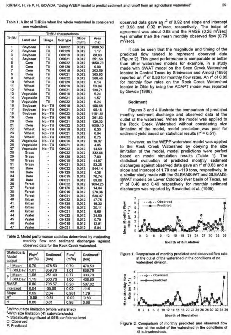
From the analysis of the GIS data base, it was found the minimum, maximum and mean elevation in the watershed were 208, 299, and 261 meters, respectively. The major soil map unit in the watershed was OH022 which covers 68% of the total area. From the land use layers, it was found that major crops in the watershed were soybean and corn which covered about 36% and 24% of the total area, respectively. Table 1 presents a list of THRUs found on the whole watershed and their characteristics. When the whole watershed was divided into 41 subwatersheds, THRUs found on the each sub-watersheds changed from 9 to 18.
flow
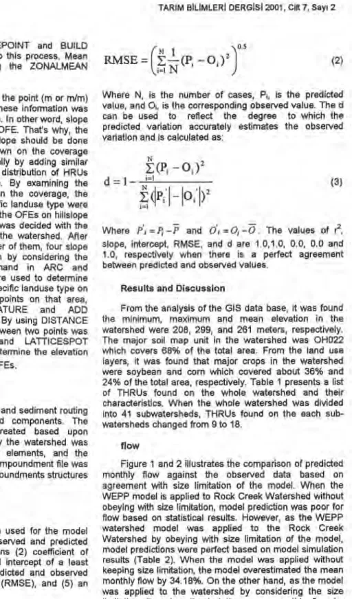
Figure 1 and 2 illustrates the comparison of predicted monthly flow against the observed data based on agreement with size limitation of the model. When the WEPP model is applied to Rock Creek Watershed without obeying with size limitation, model prediction was poor for flow based on statistical results. However, as the WEPP watershed model was applied to the Rock Creek Watershed by obeying with size limitation of the model, model predictions were perfect based on model simulation results (Table 2). When the model was applied without keeping size limitation, the model overestimated the mean monthly flow by 34.18%. On the other hand, as the model was applied to the watershed by considering the size limitation, it underestimated the mean monthly flow by 2.54%.
Statistical evaluation of predicted mean monthly flow rates against observed data in the conditions of obeying with size limitation gaye an r2 of 0.59 and slope and intercept of 0.69 and 0.04 m 3/sec, respectively. The d was about 0.86 and the RMSE (0.80 m 3/sec) was bigger than the mean monthly observed flow (0.79 m 3/sec). This statistical results showed that the WEPP watershed model could not applied on a watershed without considering the size limitation. When the model was applied by considering the size limitation of the model, statistical evaluation of predicted mean monthly flow rates against
)0.5
0 2 4 6 8 10 12 14 16 18 20 22 24 26 28 30 32 34 36 M onth of Sim ulation
Observed predicted 6 5 _ 4 3 2- Table 1. A list of THRUs when the whole watershed is considered
one watershed.
THRU
THRU characteristics
Land use Tillage Soil type Slope
(m/m) Ama (ha) 1 Soybean o o o o o o o o o o o o z zz zz z zzzzzz OH022 0.012 1008.56 2 Soybean OH129 0.012 1.17 3 Soybean OH019 0.012 88.60 4 Soybean OH021 0.012 251.58 5 Corn OH022 0.012 1050.73 6 Corn OH129 0.012 0.09 7 Corn OH019 0.012 203.59 8 Corn OH021 0.012 365.93 9 Wheat OH022 0.012 366.46 10 Wheat OH129 0.012 0.14 11 Wheat OH019 0.012 59.94 12 Wheat OH021 0.012 139.71 13 Vegetable OH019 0.012 5.24 14 Vegetable OH021 0.012 1.57 15 Vegetable OH022 0.012 6.24 16 Soybean OH019 0.012 158.68 17 Soybean OH021 0.012 95.18 18 Soybean OH022 0.012 1101.61 19 Corn OH019 0.012 261.62 20 Corn OH021 0.012 126.33 21 Corn OH022 0.012 1009.10 22 Wheat OH019 0.012 0.30 23 Wheat OH021 0.012 0.04 24 Wheat OH022 0.012 0.75 25 Vegetable OH019 0.012 16.37 26 Vegetable OH021 0.012 4.05 27 Vegetable OH022 0.012 14.50 28 Grass OH022 0.012 332.88 29 Grass OH129 0.012 7.90 30 Grass OH019 0.012 44.97 31 Grass OH021 0.012 53.25 32 Bare OH022 0.012 544.14 33 Bare OH129 0.012 4.38 34 Bare OH019 0.012 70.74 35 Bara OH021 0.012 89.88 36 Forest OH022 0.012 1094.25 37 Forest OH129 0.012 14.04 38 Forest OH019 0.012 270.36 39 Forest OH021 0.012 530.47 40 Urban OH022 0.012 47.75 41 Urban OH129 0.012 16.30 42 Urban OH019 0.012 20.11 43 Urban OH021 0.012 6.65 44 Water OH022 0.012 24.00 45 Water OH129 0.012 0.79 46 Water OH019 0.012 12.91 47 Water OH021 0.012 5.84
Table 2. Model performance s atistics determined by evaluating monthly flow and sedimen discharges against observed data for the Rock Creek watershed.
Statistics & Model out,ut Flowl (m 3/s) Sediment' (ton) Flow2 (m 3/s) Sediment2 (ton) O Mean 0.79 478.53 0.79 478.53 Std.Dev 1.01 859.76 1.01 859.76 P Mean 1.06 251.40 0.77 333.70 Std.Dev i 1.15 300.70 1.00 438.60 RMSE I 0.80 706.57 0.28 507.02 I ntercept 0.04 -35.00 0.02 -119 Slope 0.69 . . 2.04 _ 0.981 1.79 R2 0.59 0.51 0.92 -0.83 d 0.86 0.61 0.98 0.88
1-Without size limitation (whole watershed)
2-With size limitation (41 subwatersheds) *- Statistically signifıcant at 95% confidence level O: Observed
P: Predicted
observed data gaye an r 2 of 0.92 and slope and intercept of 0.98 and 0.02 m 3/sec, respectively. The index of agreement was about 0.98 and the RMSE (0.28 m 3/sec) was smaller than the mean monthly observed flow (0.79 m3/sec).
It can be seen that the magnitude and timing of the predicted flow tended to represent observed data (Figure 2). This good performance is comparable or better than other watershed models for example, in a study made with SWAT model on the Seco Creek Watershed located in Central Texas by Srinivasan and Arnold (1995) reported an r2 of 0.86 for monthly flow rates. An r2 of 0.85 for monthly flow rates on the Rock Creek Watershed located in Ohio by using the ADAPT model was reported by Gowda (1996).
Sediment
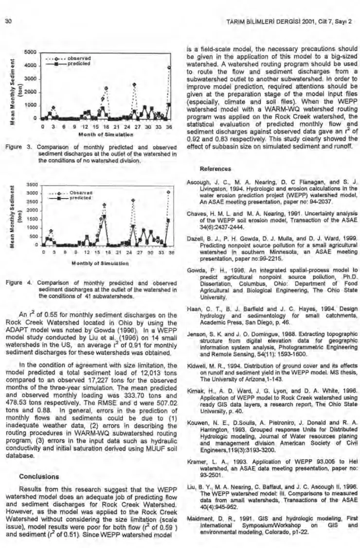
Figures 3 and 4 illustrate the comparison of predicted monthly sediment discharge and observed data at the outlet of the watershed. When the model was applied to the Rock Creek Watershed without considering size limitation of the model, model prediction was poor for sediment yield based on statistical results (r 2 = 0.51).
However, as the WEPP watershed model was applied to the Rock Creek Watershed by obeying the size limitation of the model, model predictions were perfect based on model simulation results (Table 1). The statistical evaluation of predicted monthly sediment discharges against observed data gaye an r 2 of 0.83 and a slope and intercept of 1.79 and -119 tons, respectively. In a similar study made with the WT and GLEAMS-SWAT models on Lower Colorado river basin of Texas, an r2 of 0.40 and 0.46 respectively for monthly sediment discharges was reported by Rosenthal et al. (1995).
0 LL 0 2 (7ı w 0 3 6 9 12 15 18 21 24 27 30 33 36 M o nth of Sim ulation
Figure 1. Comparison of monthly predicted and observed flow rate
at the outlet of the watershed in the conditions of no
watershed division.
Figure 2. Comparison of monthly predicted and observed flow
rate at the outlet of the watershed in the conditions of 41 subwatersheds.
cu 4000 E • 3000 >, o 2 e 2 0 3 6 9 12 15 18 21 24 27 30 33 36 M o nth of Sim ulation E o o 2 c 3500 3000 2500 2000 1500 1000 500 0 o- - Observed predicted
Figure 3. Comparison of monthly predicted and observed sediment discharges at the outlet of the watershed in the conditions of no watershed division.
is a field-scale model, the necessary precautions should be giyen in the application of this model to a big-sized watershed. A watershed routing program should be used to route the flow and sediment discharges from a subwatershed outlet to another subwatershed. In order to improve model prediction, required attentions should be giyen at the preparation stage of the model input files (especially, climate and soil files). When the WEPP watershed model with a WARM-WQ watershed routing program was applied on the Rock Creek watershed, the statistical evaluation of predicted monthly flow and sediment discharges against observed data gave an r 2 of 0.92 and 0.83 respectively. This study clearly showed the effect of subbasin size on simulated sediment and runoff.
References
O 3 6 9 12 15 18 21 24 27 30 33 36
M onthly of Simulation
Figure 4. Comparison of monthly predicted and observed sediment discharges at the outlet of the watershed in the conditions of 41 subwatersheds.
An r2 of 0.55 for monthly sediment discharges on the Rock Creek Watershed located in Ohio by using the ADAPT model was noted by Gowda (1996). In a WEPP model study conducted by Liu et al. (1996) on 14 small watersheds in the US, an average r2 of 0.91 for monthly sediment discharges for these watersheds was obtained.
In the condition of agreement with size limitation, the model predicted a total sediment load of 12,013 tons compared to an observed 17,227 tons for the observed months of the three-year simulation. The mean predicted and observed monthly loading was 333.70 tons and 478.53 tons respectively. The RMSE and d were 507.02 tons and 0.88. In general, errors in the prediction of monthly flows and sediments could be due to (1) inadequate weather data, (2) errors in describing the routing procedures in WARM-WQ subwatershed routing program, (3) errors in the input data such as hydraulic conductivity and initial saturation derived using MUUF soil database.
Conclusions
Results from this research suggest that the WEPP watershed model does an adequate job of predicting flow and sediment discharges for Rock Creek Watershed. However, as the model was applied to the Rock Creek Watershed without considering the size limitation (scale issue), model results were poor for both flow (r2 of 0.59 ) and sediment (t2 of 0.51). Since WEPP watershed model
Ascough, J. C., M. A. Nearing, D. C Flanagan, and S. J. Livingston, 1994. Hydrologic and erosion calculations in the water erosion prediction project (WEPP) watershed model, An ASAE meeting presentation, paper no: 94-2037.
Chaves, H. M. L. and M. A. Nearing, 1991. Uncertainty analysis of the WEPP soil erosion model, Transaction of the ASAE 34(6):2437-2444.
Dazell, B. J., P. H. Gowda, D. J. Mulla, and D. J. Ward, 1999. Predicting nonpoint source pollution for a small agricultural watershed in southern Minnesota, an ASAE meeting
presentation, paper no:99-2215.
Gowda, P. H., 1996. An integrated spatial-process model to predict agricultural nonpoint source pollution, Ph.D. Dissertation, Columbus, Ohio: Department of Food Agricultural and Biological Engineering, The Ohio State University.
Haan, C. T., B. J. Barfield and J. C. Hayes, 1994. Design hydrology and sedimentology for small catchments, Academic Press, San Diego, p. 46.
Jenson, S. K. and J. O. Domingue, 1988. Extracting topographic structure from digital elevation data for geographic information system analysis, Photogrammetric Engineering and Remote Sensing, 54(11): 1593-1600.
Kidwell, M. R., 1994. Distribution of ground cover and its effects on runoff and sediment yield in the WEPP model. MS thesis, The University of Arizona,1-143.
Kirnak, H., A. D. Ward, J. G. Lyon, and D. A. White, 1996. Application of WEPP model to Rock Creek watershed using ready GIS data layers, a research report, The Ohio State University, p. 40.
Kouwen, N. E., D.Soulis, A. Pietroniro, J. Donald and R. A. Harrington, 1993. Grouped response Units for Distributed Hydrologic modeling, Journal of Water resources planing and management division American Society of Civil Engineers,119(3):3193-3200.
Kramer, L. A., 1993. Application of WEPP 93.005 to Hel watershed, an ASAE data meeting presentation, paper no: 93-2501.
Liu, B. Y., M. A. Nearing, C. Baffaut, and J. C. Ascough Il, 1996. The WEPP watershed model: III. Comparisons to measured data from small watersheds, Transactions of the ASAE 40(4):945-952.
Maidment, D. R., 1991. GIS and hydrologic modeling, First
International Symposium/Workshop on GIS and environmental modeling, Colorado, p1-22.
Rango, A., A. Feldman, T. S. George III, R. M. Ragan, 1983. Effective use of landsat data in hydrologic models, Water Resources Bulletin, 19(2):165-174.
Rosenthal, W.D., R. Srinivasan, and J.G. Arnold, 1995. Alternative river management using a linked GIS-hydrology model, Transaction of the ASAE 38(3):783-790.
Savabi, M. R., W. J. Rawls, W. J. Williams, J. R., and A. D.Nicks, 1989. Water Erosion Prediction Project (WEPP) water balance submodel, An ASAE meeting presentation, paper no: 89-2672.
Searing, M. L., and A. Shirmohammadi, 1993. Utilizing GIS and GLEAMS to prescribe best management practice's for reducing nonpoint source pollution, an ASAE meeting presentation, paper no: 93-3558.
Srinivasan, R., and J. G. Arnold, 1995. Integration of a besin-scale water quality model with GIS, Water rescues Bulletin, 30(3):453-462.
Tim, U. S., S. Mostaghimi, and V. O. Shanholtz, 1992. Identifıcation of critical nonpoint pollution source areas using geographic information systems and water quality modeling, Water Resources Bulletin, 28(5):877-887.
Van Deventer, A. P., A. D. Ward, P. H. Gowda, and J. G. Lyon, 1994. Using thematic mapper data to identify contrasting soil plains and tillage practices, Manuscript, Ohio Agricultural Research and Development Journal Article No: 131-93.
WEPP, 1995. USDA-Water Erosion Prediction Project, WEPP user summary conference, August 9-11, Des Moines, lowa.