Isı Bilimi ve Tekniği Dergisi, 37, 2, 75-88, 2017 J. of Thermal Science and Technology ©2017 TIBTD Printed in Turkey ISSN 1300-3615
A NEW METHOD FOR THE OPTIMIZATION OF INSULATION THICKNESS FOR
RADIANT WALL HEATING SYSTEMS
Aliihsan KOCA*, Gürsel ÇETİN** and Eser VELİŞAN***
*Fatih Sultan Mehmet Vakıf Üniversitesi, Mühendislik Fakültesi, 34445 İstanbul, Türkiye, [email protected] ** Mir Araştırma ve Geliştirme A.S., 34220 Istanbul, Turkey, [email protected]
*** Mir Araştırma ve Geliştirme A.S., 34220 Istanbul, Turkey, [email protected] (Geliş Tarihi: 10.11.2016, Kabul Tarihi: 07.02.2017)
Abstract: In this study we proposed a new modified New Degree-Day Method (NDDM) for the optimization of insulation thickness of the wall where the radiant panels are mounted (WMRP) in which heat generation inside the wall is considered. The existing Standard Degree-Day Method (SDDM) is not applicable to estimate the optimum insulation thickness for the buildings where the WMRP is mounted. Because SDDM method uses indoor air temperature as a base temperature, hence heat generation through the WMRP cannot be taken into account. In the new method, important parameters were obtained from the series of the CFD analysis for different thermal transmittance coefficient (U) and outdoor air temperature (To) values are used to create an empirical equation for the estimation of Tp (new base temperature) with the multiple polynomial regression method. Then the numerical results were validated with experimental results which were obtained from the real-size test chamber. Using the new method optimum insulation thickness, net energy saving and payback periods for radiant wall heating systems were calculated (for Istanbul climate) and compared with the results which were obtained using the standard degree-day method (SDDM). The results showed that, the SDDM significantly lower (85-95%) estimates the optimum insulation thickness and can’t be used for the buildings where the WMRP is used. The new method can be used for radiant wall heating systems where the performance of radiant heating systems is significantly affected by the insulation capabilities and has a great importance in the sizing process of the radiant systems.
Keywords: Radiant wall heating; Optimum insulation thickness; New degree-day method.
IŞINIMLA DUVARDAN ISITMA SİSTEMLERİNDE YALITIM KALINLIĞI
OPTİMİZASYONUNDA KULLANILABİLECEK YENİ BİR YÖNTEM
Özet: Bu çalışmada ışınım ısıtma panellerin kullandığı duvarlardaki yalıtım kalınlığının optimizasyonu için, duvarlardaki ısı üretimini dikkate alan, yeni bir derece-gün yöntemi (NDDM) geliştirilmiştir. Standard Derece-Gün Yöntemi (SDDM) temel sıcaklık olarak mahal hava sıcaklığını dikkate almakta ve duvara monte edilmiş ışınım panellerindeki ısı üretimini dikkate alamamaktadır. Bu yüzden standart yöntem ile ışınım panellerin bulundugu duvarlar için yalıtım kalınlığı optimizasyonu yapmak imkansızdır. Önerilen yeni metotta kullanılan yeni temel sıcaklık değerinin (Tp) elde edilmesinde kullanılan ampirik ifade (3. dereceden polinom) farklı yapı ısı geçirgenlik katsayısı (U) ve farklı dış hava sıcaklıkları (To) parametreleri için sayısal analizlerden elde edilmiştir. Daha sonra sayısal çalısmaların sonuçları aynı şartlarda yürütülen gerçek ölçekli deney sisteminde doğrulanmıştır. İstanbul iklim şartları için yeni yöntem ve eski yontem kullanılarak ideal yalıtım kalınlıkları, enerji tasarrufları ve geri dönüş süreleri hesaplanmış, iki yöntemden elde edilen sonuçlar kıyaslanmiştir. Sonuçlara göre eski yöntemle hesaplanan ideal yalıtım kalınlığı yeni yöntemden elde edilen değerin çok altında (%85-95) kalmaktadır. Bu yüzden standart yöntemin ısı üretimi olan duvarlarda kullanılmasının mümkün olmadığı görulmüştür. Önerilen yeni yöntem ise, ışınımla ısıtma sistemlerinin projelendirilmesinde önemli bir kriter olan ısı kayıplarının hesaplanması ve ideal yalıtım kalınlığının belirlenmesinde kullanılabilecektir.
Anahtar Kelimler: Işınımla duvardan ısıtma, Optimum yalıtım kalınlığı, Yeni derece-gün yöntemi. NOMENCLATURE
A Area [m2]
CA Annular heating cost [TL/yr]
Cf Fuel cost [TL/kg]
Ctins Insulation cost per unit area [TL/m2]
hi Inner heat transfer coefficient [W/m2.K]
ho Outer heat transfer coefficient [W/m2.K]
Hu Lower heating value of the fuel [j/kg]
k Heat conduction coefficient [W/m.K] mf Annular fuel mass [kg]
Ri Inside air film thermal resistance [m2.K/W]
Ro Outside air film thermal resist. [m2.K/W]
Rw Total thermal resistance [m2.K/W]
Tb Base temperature [°C]
Ti Indoor air temperature [°C]
Tp WMRP backside temperature [°C]
Tsi Inner surface temperature of the wall [°C]
Tso Outer surface temperature of the wall [°C]
q′′ Heat flux [W/m2]
U Coefficient of thermal trans. [W/m2.K]
x Insulation thickness [m]
xop Optimum insulation thickness [m]
η Efficiency of heating system [%] Abbreviations
CFD Computational Fluid Dynamics
DD Degree-Day
HVAC Heating Ventilating Air Cond. LCCA Life Cycle Cost Analysis NDDM New Degree Day Method PBP Pay Back Period
SDDM Standard Degree-Day Method WMRP Wall-Mounted Radiant Panel MPR Multiple Polynomial Regression INTRODUCTION
It is a fact that energy consumption is one of the world’s biggest problems since energy need is increasing proportionally to the population and conventional sources are diminishing evenly. As a result of this, the International Energy Agency (2013) predicts an increase in global energy consumption by 56% from 2010 to 2040. For the present, fossil fuels are used as major energy sources but they will not able to meet energy requirement in the near future. Thus, it is important to ensure energy efficiency when using fossil fuels and place an emphasis on finding alternative energy solutions. Energy management and efficiency will be an important matter in the coming years. Therefore developing systems which promote energy saving is inevitable. Although the economy has been growing gradually in Turkey as well as energy demand and energy policy is heavily dependent on imported energy. The government invested 25$ billion in energy production between the years 2002 and 2011, but still Turkey has to import 71% of energy needs. According to the Energy and Natural Resources Ministry of Turkey (2013) 31% of Turkey’s energy is being used in buildings. This high percentage is due to the fact that most buildings do not meet general energy efficiency criteria such as thermal insulation requirements for external walls. Thermal insulation is an easy and applicable method to increase energy efficiency by means of decreasing the heat flux from indoor to outdoor and vice versa (Çomaklı and Yüksel, 2003).
Insulation thickness is a parameter which balances investment and operational cost. In the literature, there are many studies which have been investigating how to determine optimum insulation thickness (Yıldız et al., 2008; Dikmen, 2011; Bolattürk and Dağıdır, 2013; Kaynaklı, 2013; Kaya et al., 2016; Duman et al., 2015). Çomaklı and Yüksel (2004) used life cycle cost analysis (LCCA) based on the degree day method for calculation of optimum insulation thickness and annual energy savings of some cities from 4th climatic region of Turkey and also they discussed the subject from an
environmental point of view. Optimum insulation thickness of Denizli region for different fuel types and different insulation materials was obtained by Dombaycı et al. (2006) by using the standard degree-day method. Differently, Arslan and Köse (2006) also took into account the effect of condensed vapor within the standard degree day method. Further, Sisman et al. (2007) calculated optimum insulation thickness of roofs for different degree-day regions of Turkey. Kaynaklı (2008) chose Bursa as a model city and evaluated residential energy requirement for heating season and calculated optimum insulation thicknesses for different types of fuels. Bolattürk (2008) calculated the optimum insulation thickness using his method and compared the results with the standard heating degree-hour method. Ucar (2010) determined optimum insulation thicknesses for four different climatic regions of Turkey by using exergy analysis method. Optimum insulation thicknesses and energy savings were also studied by Ucar and Balo (2010) for different regions of Turkey. Ozkan and Onan (2011) considered effects of glazing areas on the optimum insulation thickness. Ozel (2011) determined optimum insulation thickness by using a dynamic method. Kaynaklı (2012) reviewed the existing studies with focusing on reported optimum insulation thickness results. Ekici et al. (2012) calculated optimum insulation thickness using different wall structures and fuels for different regions of Turkey. De Rosa et al. (2014) evaluated energy demand by a method which combines dynamic model based on the lumped capacitance approach and electrical analogy method.
Radiant heating systems are different from typical HVAC systems because they heat surfaces rather than air and can save large amounts of energy while providing higher levels of thermal comfort. The radiant heating system consists of large radiant heat transfer surfaces can be installed on room walls, floors or ceilings. A conditioned surface is called as a radiant system if 50% or more of the designed heat transfer on the temperature-controlled surface takes place by thermal radiation. Radiant heating systems are quite convenient alternatives to the traditional HVAC systems. They reduce energy consumption because of low-temperature heating and high temperature cooling operations. In the literature heat transfer, thermal comfort performances and energy efficiency capabilities of these kinds of systems have been studied in detailed (Kilkis, 2006; Tye-Gingras and Gosselin, 2012; Seyam et al., 2014; Bojic et al., 2015; Rehee and Kim, 2015; Jeong et al., 2013; Stetiu, 1999; Franc, 1999; Miriel et al., 2002; Koca et al., 2016; Koca et al., 2014; Koca et al., 2013; Koca, 2011; Erikci Çelik et al., 2016; Kanbur et al., 2013; Acikgoz and Kincay, 2015). Therefore this proven technology should be disseminated in Turkey to achieve energy efficiency goals of the country.
In the literature, not many studies available dealt with the optimization of insulation thickness for radiant heating cooling systems. There is only one study (Cvetkovi and Bojic, 2014) available in the literature, in which the investigators used Energy Plus© software to
77 evaluate the energy consumption of the simulate building. They reported that radiant wall insulation requires a higher insulation thickness when compared with other radiant systems. Moreover the thickness of thermal insulation is the highest for the location where the radiant panels are located. The house with the optimal thermal insulation thickness has significant energy saving compared to house with older customary thermal insulation (Cvetkovi and Bojic, 2014). But in their study, they conducted the simulations according to Serbian climate conditions without any experimental validation. Moreover, they did not compare the classical methods with their newly reported results.
In most of the aforementioned studies researchers dealt only with theoretical examination using either degree-day or hourly-based methods without any experimental validation. As a result of this the results of these studies are not valid for the radiant heating systems, since the indoor air temperatures are taken into account as a heat source (or base temperature). In radiant heating systems there is no indoor heat loss through the walls where the radiant heating panels are mounted. In such cases heat loss occurs through the panel backside surfaces. Therefore, in this study we propose a new method to evaluate the optimum insulation thicknesses of radiant wall heating systems that takes into account the radiant panel backside temperature as a heat source where the huge amount of heat leakage occurs. For this reason, our first goal is to evaluate optimum insulation thicknesses for radiant wall heating systems since the performance of radiant heating systems is significantly affected by the insulation capabilities and has a great importance in the sizing process of the radiant systems. In the new method important parameters, that were obtained from a series of the CFD analysis for different thermal transmittance coefficient (U) and outdoor air temperature (To) values, are used to create an empirical correlation for the estimation of Tp (the new base temperature) with multiple polynomial regression method. A new experimental test set-up which simulates typical conditions of occupancy in an office or residential room was used for the validation of the computational results. Then serial CFD analyses were conducted to create a new correlation for the estimation of the base temperature (Tp) with multiple polynomial regression method (MPR). Based on the new base temperature, LCCA based Standard Degree-Day Method (SDDM) is adjusted for Wall-Mounted Radiant Panel (WMRP) and created a New LCCA based Degree-Day Method (NDDM). Using the new method optimum insulation thickness, net energy saving and payback periods for radiant wall heating systems were calculated for the city of Istanbul and compared with the results which were obtained using the standard degree-day method (SDDM).
NUMERICAL MODEL
In this work, a numerical model was developed using the commercial CFD package ANSYS-FLUENT© Version 15 to simulate the WMRP. Fluent uses a control-volume-based technique to convert an inclusive scalar transport
equation to an algebraic equation that is solved numerically. The steady simulations were performed with the software, using the coupled double precision solver. Physical Model
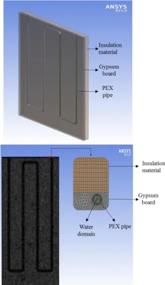
A 3D model that has the same dimensions as the experimental set-up (1.2 m in height, 0.6 m in length) was used for the simulations. The pipe in the panel which is made of cross-linked polyethylene (PEX) has 10.1 mm outer diameter and 1.1 mm thickness with 150 mm pipe spacing. The gypsum board which is exposed to the inside room has 1.5 cm thickness. EPS (Expanded Polystyrene) was used as an insulation material which has a coefficient of thermal transmittance value of 0.039 W/m.K (at 25˚C). To decrease the mesh number and precisely solve the heat loss from the WMRP, experimental room domain wasn’t considered in our numerical model. Instead, average total heat transfer coefficient – comprised of the radiation and convection – was implemented as a surface boundary condition. The implemented average total heat transfer coefficient was obtained experimentally (using the same test chamber in this study) in our previous study (Koca et al., 2014) using different WMRP surface temperatures and which are valid for wide range (25 - 45 °C) of WMRP surface temperature. According to the results of Koca et al. (2014), the measured average values of radiant heat transfer coefficient is about 5.46 W/m2.K and convection
heat transfer coefficient is about 2.32 W/m2.K resulting
in an average total heat transfer coefficient of 8.33 W/m2.K – which was considered in this study. Obtained
average total heat transfer coefficient for wall (8.33 W/m2.K) is compatible with the ones typically shown in
standards of EN 15377-1 (2008) and EN 1264-5 (2008).
Computational Domain, Mesh and Mesh
Independency Analysis
The computational mesh was generated using tetra and hexahedral elements with ANSYS Meshing tool. In order to accurately resolve the solution fields in the vicinity of the heat transfer surface between pipe and the surrounding interface, the mesh was refined at the area where the heating pipes are embedded. The grid was fine enough for the other areas to solve the simple heat conduction problem. A sample of the computational model and grid was shown in Fig. 1. Before the computations, a grid independence study was carried out to ensure the results’ accuracy. Eight different mesh configurations (varies from 1M to 27M) were analyzed for same boundary conditions and the calculated panel backside surface temperature (Tp) –
which is our main parameter – was compared. As shown in Fig. 2, at the range between the first and third configurations of the results slightly vary with the grid resolution but after the fourth mesh configuration, Tp
tends towards constant. So after that point the results can be considered grid independent. In regard to this mesh independence results, simulations were carried
out with the mesh configuration which has 6.5M elements and average skewness value of 0.20.
Figure 1. CAD model of the panel (left) and computational mesh grids (right)
Figure 2. Mesh independence study
Solution Methods and Procedure
3D, steady-state, CFD analysis were performed by using ANSYS FLUENT 15©. Mass, momentum and
energy conservation equations were solved numerically. As main boundary condition, WMRP surface was set as mixed (radiation and convection) heat transfer surface, where the average total heat transfer coefficient (sum of radiation and convection) was defined as the value of 8.33 W/m2.K (radiant and
convective heat transfer coefficients were obtained from our previous work done by Koca et al., 2014). The other side walls were set as adiabatic boundary conditions. The backside of the panel was set to the convection surface having the certain value of total heat transfer coefficient of 25 W/m2.K.
The outside air temperature of the WMRP – which is exposed to outside conditions – was set at certain values and studied as a parameter in the simulations. The indoor room temperature (Ti) was defined constant
as 15°C for all cases. Inlet water mass flow rate was defined as constant at the value of 0.04 kg/s (Reynolds number is 4200). Therefore a turbulence model (Realizable k-ε model) was chosen for the calculations. Also enhanced wall treatment was implemented for the heat transfer surface where the y+ value is varied
between 1 and 5. Among the different code options, Second Order Upwind law interpolation scheme and the discretized equations were chosen and numerically solved by the SIMPLE algorithm. In the present work, all the solutions were considered to be fully converged when the sum of residuals was below 1×10⁻⁴.
Multiple simulations were conducted by varying outdoor air temperature (To) and insulation thickness
(∆p) of the WMRP. Outdoor air temperature values
between -15 °C and +18 °C (34 different outdoor temperatures increased numerically between -15 °C and +18 °C within a value of around 1 °C) were set as a boundary conditions of the WMRP while the insulation thickness of the panel was varied between 0 - 16 cm (16 different insulation thickness with 1 cm variation). On the basis of the obtained simulations, the backside surface temperatures of WMRP (Tp) were evaluated
using area-weighted-average method (cell-centered) and the results are presented in Table 1.
In the table, values of total U (overall coefficient of thermal transmittance of WMRP) and outdoor air temperature (To in °C) are the input parameter, WMRP
backside temperature (Tp in °C) is the output parameter
79
Table 1. Result summary of the numerical simulations
To UNDDM x Tp To UNDDM x Tp To UNDDM x Tp To UNDDM x Tp -15 0.23 16 20.7 2 0.23 16 23.1 18 0.23 16 25.8 1 0.23 16 22.9 -14 0.24 15 20 3 0.24 15 23 17 0.24 15 25.6 0 0.24 15 22.5 -13 0.26 14 19.8 4 0.26 14 23 16 0.26 14 25.3 -1 0.26 14 22.1 -12 0.28 13 19.6 5 0.28 13 22 15 0.28 13 24 -2 0.28 13 21.6 -11 0.30 12 19.4 6 0.30 12 22.9 14 0.30 12 24.6 -3 0.30 12 21.1 -10 0.32 11 19.1 7 0.32 11 22.9 13 0.32 11 24.2 -4 0.32 11 20.5 -9 0.35 10 18.8 8 0.35 10 22.8 12 0.35 10 23.8 -5 0.35 10 19.8 -8 0.38 9 18.5 9 0.38 9 22.8 11 0.38 9 23.3 -6 0.38 9 19 -7 0.42 8 18.1 10 0.42 8 22.7 10 0.42 8 22.7 -7 0.42 8 18.1 -6 0.47 7 17.6 11 0.47 7 22.6 9 0.47 7 22 -8 0.47 7 17 -5 0.53 6 17 12 0.53 6 22.5 8 0.53 6 21.2 -9 0.53 6 15.8 -4 0.61 5 16.4 13 0.61 5 22.4 7 0.61 5 20.3 -10 0.61 5 14.3 -3 0.72 4 15.7 14 0.72 4 22.3 6 0.72 4 19.2 -11 0.72 4 12.6 -2 0.88 3 14.7 15 0.88 3 22.1 5 0.88 3 17.7 -12 0.88 3 10.3 -1 1.12 2 13.5 16 1.12 2 21.9 4 1.12 2 15 -13 1.12 2 7.6 0 1.56 1 11.9 17 1.56 1 21.6 3 1.56 1 13.6 -14 1.56 1 3.9 1 2.55 0 9.8 18 2.55 0 21.3 2 2.55 0 10.3 -15 2.55 0 -1.2 METHODOLOGY
A New Degree-Day Calculation Method for Wall-Mounted Radiant Panels
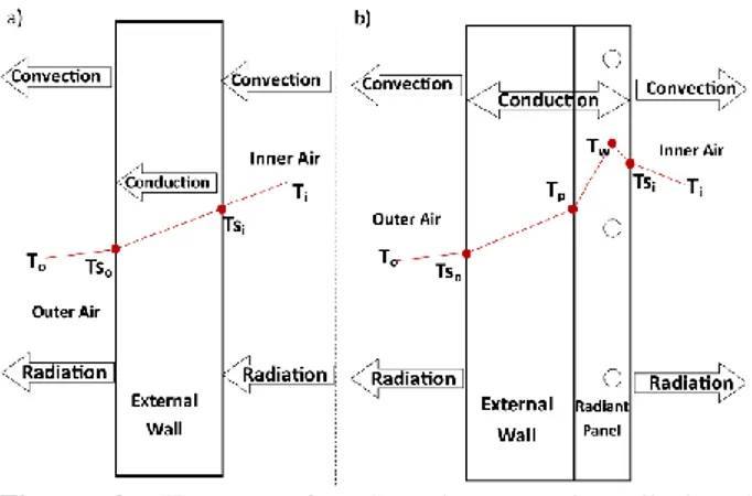
In (SDDM), degree-day value (DD) is calculated using inner and outer air temperatures for a fixed base temperature. This method cannot be applied for buildings heated by WMRP due to the fact that WMRP has different heat transfer characteristic comparing to the conventional systems. Because in these kinds of systems, heat source is part of the wall structure and this causes two-way conduction in the structure. However, as shown in Fig. 3, the temperature gradient from inner surface temperature (Tsi) to outer air temperature (To) in
conventional systems is similar to the temperature gradient (from backside temperature, Tp to outer air
temperature, To) in radiant systems. Therefore, a
correlation for the evaluation of Tp which is based on the
To and overall heat transfer coefficient of wall (U) was
obtained using a numeric and statistical methods.
Figure 3. Heat transfer through external wall in a) conventional system b) WMRP system
Moreover base temperature (Ti in Fig. 3)was defined as
15°C for the calculation of degree-day value in SDDM whereas internal heat sources (human, electronic devices etc.) exist. Eqs. 1 and 2 show the general calculation procedure of the DD value:
f(D) = {T 0 , Tb< To
p(U, To) − To , Tb≥ To (1)
DD = ∑ND=1f(i) (2) 25-year averages of daily air temperatures were used to calculate the degree-day value and the degree day value is a series sum of day 1 to day 365 as a function of Tp.
Also Tp is a function of x, which was obtained from
regression of CFD results.
Multiple Polynomial Regressions
Multiple polynomial regressions, is a statistical approach for modeling of the relationship between a dependent variable and independent variables. WMRP backside temperature (Tp)values were obtained from series of the
CFD analysis for different thermal transmittance coefficient (U) and outdoor air temperature (To)values
were used to create an empirical equation for the estimation of Tp with multiple polynomial regression
method (MPR) where the Newton-Raphson method was implemented. In MPR, 3rd degree of the polynomial
equation (Eq. 3) was chosen in which the results were best yielded (correlation coefficient (R2) is 0.998 and
Residual Sum of Squares (RSS) is 0.74).
Tp= A To3+ BTo2U + CToU2+ DU3+ ETo2+ FToU +
GU2+ HT
o+ IU + J (3)
DD = ∑ND=1A To3+ BTo2U + CToU2+ DU3+ ETo2+
FToU + GU2+ (H−1)To+ IU + J (4)
The constant coefficients of the above equations are given in Table 2.
Table 2. Coefficients of the polynomial equation
A B C D E
-1.40·10-4 - 2.36·10-4 - 9.61·10-2 - 1.27 1.16·10-1
F G H I J
6.16·10-1
Calculation of Optimum Insulation Thickness Using New and Standard Degree Day Methods
Eqs. 5-6 and Eqs. 9-15 are common for both new and standard methods. Calculation method of overall heat transfer coefficient (U) is similar both in NDDM and SDDM. Nevertheless in NDDM inner heat transfer coefficient (hi) and thermal resistance of panel (Rp) are
not included into the equation since these parameters have already been taken into account in the CFD calculations and embedded into the proposed equation of Tp (Eq. 3).
The heat loss per unit area of external walls is given by: Q = U(Tb− To) (5)
Annual heat loss per unit area from external walls (𝑞′′)
in the terms of degree-days is given by:
q′′= 86400 ∙ DD ∙ U (6)
Overall heat transfer coefficient (U) and equivalent thermal resistance of wall (𝑅𝑡𝑤) were calculated using
the Eqs. 7-8. Whereby, Eq. 8a and Eq. 8b were used to calculate the U values of interest for SDDM and NDDM respectively: Rtw= Rw+ Rins+ Ri+ Ro (7) USDDM= 1 Rw+xk+ho1+hi1 (8a) UNDDM= 1 Rw+x k+ 1 ho (8b)
Where, Ro and Ri are the inside and outside air film
thermal resistance, Rw is the total thermal resistance of
the wall associated with the structural components of the wall and panel, hi (W/m2.K) is the inner, ho (W/m2.K) is
the outer convective heat transfer coefficients, x is the insulation thickness (m) and k (W/m.K) is the heat conduction coefficient of insulation material.
Annual energy requirement (EA) was calculated by the
Eq. 9 and it corresponds to annual heat loss. EA= mf∙ Hu∙ η =
86400∙DD (R𝑡𝑤+xk)
(9)
Where, mf (kg) is the annular fuel mass consumption, Hu
(j/kg) is lower heating value of the fuel and η (%) is the efficiency of the heating system.
Then, the annular fuel mass consumption (mf) was
obtained by dividing the annual heat loss (EA) by lower
heating value (Hu) and efficiency (η) of fuel, yields:
mf=
86400∙DD (R𝑡𝑤+xk)∙Hu∙η
(10)
If we multiply annular fuel mass consumption (mf) with
the fuel cost Cf (TL/kg), we get annular heating cost per
unit area (CA): CA= mf∙ Cf (11) CA= 86400∙DD∙Cf (R𝑡𝑤+xk)∙η∙Hu (12)
The LCCA used in this paper calculates the heating cost over the lifetime of the building. The total heating cost over a lifetime of N years is estimated in present value Turkish Liras using the PWF (Present Worth Factor). The PWF depends on the inflation rate g, and the interest rate i. The PWF, which is dependent on the inflation rate g and the interest rate i, is adjusted for inflation rate as shown below (Hasan A., 1999). The interest rate modified for inflation rate, i*, is defined by the following
equations: i∗=i−g 1+g (i>g) (13) and PWF =(1+i∗)N−1 i∗(1+i∗)N (14)
Where N is the lifetime and which is assumed to be 20 years.
Total cost (Ct) was calculated by multiplying the Present
Worth Factor (PWF) into annual heating cost (CA) and
adding the total insulation cost per unit area (𝐶𝑡𝑖𝑛𝑠).
Ct=
86400∙DD∙Cf∙PWF (Rtw+x
k)∙η∙Hu
+ Ctins (15)
The cost of investment of the insulation material is given by the following equation:
Ctins = Cins∙ x (16)
Where, Cins (TL/m2) is the cost of insulation per unit
insulation area. Therefore, the following equation gives the total cost of heating of insulated building in present sum of Turkish Liras:
Ct=
86400∙DD∙Cf∙PWF (Rtw+x
k)∙η∙Hu
+ Cins∙ x (17)
Then, the optimum insulation thickness was obtained by minimizing the total heating cost (Ct). Therefore, the
derivative of Ct with respect to the insulation thickness
(x) was taken and set equal to zero, from which the optimum insulation thickness (xop) values were derived
for SDDM (Eq. 18a) and NDDM (Eq. 18b) as follows:
dCt
dx = Cins−
86400∙DD∙Cf∙PWF∙k (k∙Rtw+x)2∙η∙Hu
81 dCt dx = ∑ Cins− ( 86400∙PWF∙Cf∙UNDDM3 k∙Hu∙η ∙ (4 ∙ D ∙ UNDDM 2+ 3 ∙ N D=1 UNDDM∙ ((C ∙ To(i)) + G) + 2 ∙ (I + (F ∙ To(i)) + B ∙ To(i)2) +
A∙To(i)3+E∙To(i)2(H−1)∙To(i)+J
UNDDM )) (18b) Eqs. 18a and 18b are different in both methods since in the NDDM Tp is a function of U (also U is a function of
x). Hence, derivation results of the Eq. 19 are different for NDDM than SDDM.
Despite of the aforementioned differences in the previous steps, the methodology of the last two steps is common for both SDDM and NDDM. A root of Eq. 19 which is the minimum point of the Eq. 18, gives the optimum insulation thickness values.
dCt
dx = 0 (19)
For the SDDM, the derivative of the Eq. 18a gives the optimum insulation thickness value, which is obtained as follows:
xopt= √
86400∙DD∙Cf∙PWF∙k
Cins∙η∙Hu − k ∙ Rtw (20)
In Eq. 18a, DD value is constant for SDDM, while the DD value in Eq. 18b for NDDM is a function of UNDDM
and accordingly function of x. For this reason in NDDM, optimum insulation thickness values were obtained using the Matlab© code because of the complicity of the
dependent variables in the Eq. 18b. In the code, to sum up the series, To values were defined as a matrix. Since
only the value of x is independent variable in the equation, the solution matrix was equalized to zero and then the values of x obtained.
Parameters used in the optimization calculations are shown in Table 3.
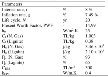
Table 3. Parameters used in the optimization of insulation thickness
Parameters
Interest rate, i % 8 %
Inflation rate, g % 7.49 %
Life cycle, N yr 20
Present Worth Factor, PWF - 14.99
h0 W/m2.K 25 Cf (N. Gas) TL/kg 1.003 Cf (Lignite) TL/kg 0.38 Hu (N. Gas) j/kg 3.46 x 10⁷ Hu (Lignite) j/kg 2.10 x 10⁷ Ƞu (N. Gas) % 93 Ƞu (Lignite) % 65 CEPS TL/m2 300 kEPS W/m.K 0.4 EXPERIMENTAL VALIDATION The Arrangement of the Test Chamber
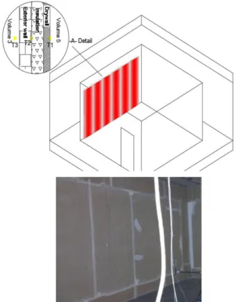
The climatic test chamber was constructed to simulate radiant wall heating system under various boundary conditions which are listed in Table 4. As seen in Fig. 4 and Fig. 5, the test chamber is composed of four zones: Ceiling (volume-4), floor (volume-3), façade (volume-2) and the tested zone (volume-1). WMRP were mounted into the tested zone which is characterized by a floor area of 16 m2 (4 m × 4 m) and an internal height of 3 m
as recommended in EN 1264-5 (2008) and BS EN 14037-5 (2016).
The wall types were chosen as the sandwich type panel with polyurethane insulation between two layers is made out of sheet steel which has engagement and locking mechanism to increase the strength. The coefficients of thermal transmittance of the wall and ceiling were decided according to Turkish Standard TS 825 (thermal insulation requirements for buildings) (2008). The enclosed volumes were conditioned with mechanical air conditioners to ensure relevant boundary conditions in the tested volume. The emissivity of the indoor wall and WMRP surfaces, were estimated by the use of an infrared thermal imaging camera and calibrated thermocouples.
First, the surface temperatures were obtained by using precise temperature sensors, and then the surface emissivity was changed in the pyrometer setup in order to get the same temperature of the analyzed surface as obtained before by the use of the temperature sensors (Olesen et al., 2000). The physical dimensions and the thermo-physical properties of the test chamber and the testing equipment meet the general requirements of the ANSI/ASHRAE Standard 138 (2005). The main difference from the standard is; to ensure appropriate boundary conditions in the tested volume, the inner surfaces in the test zone were conditioned through the surrounded volumes as they are equipped with a mechanical air conditioner whereas the ANSI/ASHRAE Standard 138 (2005) recommends directly conditioning the testing room through pipes embedded in the surfaces.
Table 4. Controlled parameters in the zones
Ceiling Floor Facade Tested zone
Temperature Range -10˚C / +40˚C +0˚C / +30˚C -10˚C / +40˚C +0˚C / +30˚C
Temperature Tolerance ± 0.5 ˚C ± 0.5 ˚C ± 0.5 ˚C ± 0.5 ˚C
Humidity Range n/a n/a %35 / %85 RH n/a
Humidity Control Steps n/a n/a %1 n/a
Humidity Tolerance n/a n/a ± % 0.5 RH n/a
Air Velocity n/a n/a 0.5 – 5 m/s n/a
Figure 5. Dimensions of the test chamber (all units are in millimeters)
The Wall Mounted Radiant Panel
The WMRP’s were manufactured for this study consist of three layers which are gypsum board, serpentine heating pipe and insulation material; from inner to outer layers. The pipe serpentine was inserted into the gypsum board. The thickness of the gypsum board is 15 mm while the panel insulation thickness is 30 mm. The serpentine has cross-linked polyethylene (PEX) pipes with a 10.1 mm external diameter and 55 mm pipe spacing. Expanded polystyrene (EPS) was used as a backside thermal insulation material which has a coefficient of thermal transmittance value of 0.040 W/m.K (at 30 °C). WMRP has the standard insulation thickness which is attached during its manufacturing process. It should be noted that, obtained optimum thickness values (xopt) in this study are an additional
insulation to be attached to the external walls.
The general dimension of the WMRP was 1.2 m in height and 0.6 m in width (same as the CFD model). The test chamber was configured with six WMRP panels which are shown in Fig. 6 but measurements were performed from one of them. Six WMRP panels were attached to the wall instead of attaching single panel, this more closely simulates typical application allowing for more realistic results.
Figure 6. Arrangement of the wall mounted radiant panel
Hydraulic Circuit of WMRP
A water conditioning system was attached to the test chamber. As shown in Fig 7, inlet water accesses the hydraulic line through the buffer tank (the water temperature is maintained by means of electrical resistances), it then comes to the four-way valve. Here, the four-way valve was placed to provide a mixture through the supply and return lines. The mixed water leaves the four-way valve such that it is equal to the desired WMRP inlet temperature and enters the pump to supply the needed pressure. Then, the water comes to the three-way valve where the mass flow rate of the water is maintained at precisely appropriate flow rate. After that, the water passes through the ultrasonic flow meter, where the volumetric flow rate was measured. The data
83 for the flow rate control was provided from an electromagnetic flow meter. Following the flow meter, the water goes through manifolds and then the WMRP facility to activate the heat transfer mechanism. After finishing the cycle in the hydraulic line, the fluid comes to the four-way valve again through the return pipeline it is mixed with the water that comes from the buffer tank if needed (to adjust the required temperature of the fluid precisely). The pipes in the water circuit are well insulated.
Figure 7. Hydraulic circuit of the test system
The Measurement Equipment and Experimental Method
The main objective of the experimental study was to validate the numerical simulation results. The most reliable analyses are those based on the measurements performed in the full scale test chamber which was described in detailed above. The measurements were carried out for the chosen representative WMRP, where the temperature transducers were inserted as described in the Fig. 3-b. For all cases, the supply water mass flow rate (0.04 kg/s) and the other environmental conditions were fixed at desired conditions. The measurements were carried out under steady conditions for variable outdoor (volume-2) air temperatures (To). The water
conditioning system was turned on to achieve the desired steady state and initial conditions and heat flow throughout the heated WMRP before collecting the experimental data. Steady state conditions were ensured after about 3-4 h in which supply water temperature and water flow rates, surface temperature of the WMRP (Tsi),
outdoor surface temperature (Tso), WMRP backside
surface temperature (Tp), outdoor air temperature (To)
and indoor air temperature (Ti) were nearly constant,
only then the tests were begun.
Indoor and surrounding volumes’ air temperatures (Ti,
To), the related surface temperatures (Tp, Tsi, Tso) water
mass flow rate, supply and return water temperatures were measured, controlled and stored for each measuring time interval (1 minute). Average test duration took around 8 h so that all important variables reached desired and steady state conditions. The temperatures of Ti, To,
Tp, Tsi, Tso were evaluated after the system reached a
steady state condition (which was characterized by physical properties that were unchanging in time). Results corresponding to average values were stored during the periods of at least 30 min in which stable conditions were observed.
Multiple tests were carried out by varying the outdoor air temperature (To1 = -3 °C, To2 = 3 °C, To3 = 5 °C) in
Volume-2. When the air and surface temperatures bands changed less than 0.1 K/min, measurements were started. In terms of the recorded measurements, the panel backside surface temperatures (Tp) were obtained and
compared with the numerical results. RESULTS AND DISCUSSION
The optimum insulation thickness (xopt) values which
were calculated by two different methods (NDDM, SDDM) for different fuels in Istanbul climate, are shown in Table 5 and described below.
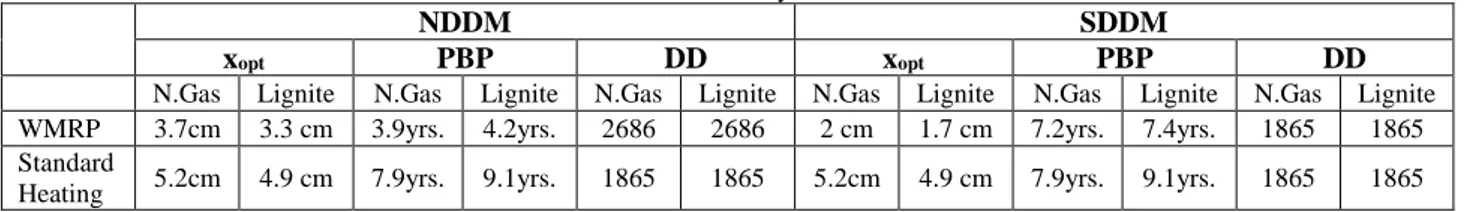
According to the general outcomes, optimum insulation thickness values which were calculated by NDDM are higher than the ones calculated by SDDM. Because, in SDDM indoor air temperature is used as a base temperature and heat production in the walls is neglected for the buildings heated by WMRP. Therefore, calculated optimum insulation thickness values from SDDM for the walls where the WMRP is mounted will be insufficient from the point of energy saving. On the other hand, optimum insulation thickness values were obtained by NDDM for a building heated by WMRP is lower than the ones obtained for standard building using the SDDM. This is because; backside insulation layer attached to the WMRP provides additional insulation to the walls, resulting in higher energy efficiency. Moreover, the payback periods (PBP) for natural gas and lignite obtained by NDDM were shorter than the ones obtained through SDDM. Accordingly, NDDM ensures better estimation of optimum insulation thickness than the SDDM, resulting in a shorter payback period.
Table 5. Summary results
NDDM SDDM
xopt PBP DD xopt PBP DD
N.Gas Lignite N.Gas Lignite N.Gas Lignite N.Gas Lignite N.Gas Lignite N.Gas Lignite WMRP 3.7cm 3.3 cm 3.9yrs. 4.2yrs. 2686 2686 2 cm 1.7 cm 7.2yrs. 7.4yrs. 1865 1865 Standard
Table 6. Validation of the numerical studies Outer Air Temperature UNDDM (W/m2.K)
Tp (°C) Error (°C)
Experimental CFD MPR CFD-Exp MPR-CFD MPR-Exp
-3 °C 0.72 15.9 15.6 15.4 -0.3 0.2 -0.5
3 °C 0.72 17.4 17.9 17.8 0.5 0.1 0.4
5 °C 0.72 18.4 18.7 18.6 0.2 0.1 0.2
Experimental Validation
The numerical model was validated with the experimental results conducted in same conditions. WMRP backside temperatures (Tp) calculated from the
simulations were compared with the experimentally evaluated results. Because Tp is the most important, new
parameter and affects the NDDM results, this validation of the Tp ensures the accuracy of the numerical results.
However to increase the accuracy of the numerical results, comparison study was done for three different outer air temperatures (To).
The comparison summary of the numerical and experimental results is shown in Table 6.
According to the comparison results of the simulated and measured Tp values; average deviation is 0.3 °C (~ 1%)
which is quite low. The maximum deviation (0.5 °C) was seen in the case where the outer air temperature (To)
value is about 3 °C. Moreover MPR and CFD results are compatible to each other and average deviation is about 0.15 °C yielded.
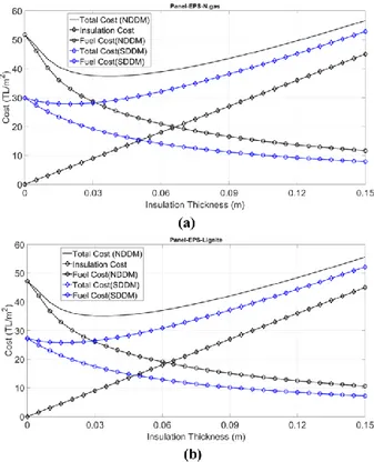
Comparison of the NDDM and SDDM Results Fig. 8 shows the variation of unit cost with respect to the insulation thicknesses (for the fuels of natural gas and lignite) that were obtained using the new (NDDM) and standard methods (SDDM). According to the results, as insulation thickness increases the heating load and accordingly heating cost decreases and vice-versa; when insulation thickness decreases, the heating load and heating cost increases. Furthermore, when the insulation thickness increases, cost of insulation also increases proportionally. When these two curves added together a total cost curve is obtained and the minimum value of this curve gives the optimum insulation thickness (xopt).
It can be seen in the Fig. 3a that for the walls where the WMRP is integrated, optimum insulation thicknesses for the usage of natural gas were obtained as 3.7 cm and 2 cm according to the NDDM and SDDM respectively. These values are 3.3 cm and 1.7 cm for the fuel of lignite (Fig 3b). Beyond these values, increasing the thickness of the insulation also increases the total cost. Table 5 shows the optimum insulation thickness results for the Istanbul for the new and standard methods described above.
With respect to the results obtained from both methods, significant difference (~85 %) in optimum insulation thicknesses is seen between the two methods. The main reason of such deviation is; heat source (WMRP) in the wall is not taken into account in the SDDM, while the
NDDM considers the interface temperature (between wall and WMRP) as a base temperature rather than indoor air temperature as well as heat generation (as mentioned above). Thus, SDDM is not convenient to estimate optimum insulation thickness for the walls where the WMRP is implemented. Nevertheless, if one wishes to use the standard method, one should double the obtained insulation thickness result from the SDDM as a safety margin.
Figure 8. Comparison of the SDDM and NDDM methods for the WMRP a) Natural Gas b) Lignite
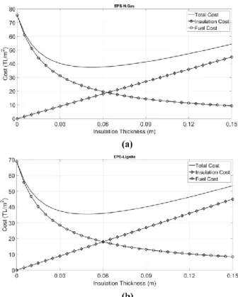
In Fig. 9, optimum insulation thickness results of SDDM for a standard building conditioned by conventional heating systems are given. As seen in the figure, optimum insulation thickness values for the fuels of natural gas and lignite are 5.2 cm and 4.9 cm respectively. If we compare the optimum insulation thickness results of conventional heating system (in SDDM) with the ones which were obtained from the case of WMRP in SDDM (corresponding to the values of 2 cm 1.6 cm), is significantly higher. Where, it can be stated that WMRP systems increase the insulation capability of buildings by means of providing extra insulation (backside insulation of the WMRP).
85
Figure 9. Optimum insulation thickness results of conventional heating systems according to the SDDM a) Natural Gas b) Lignite
Fig. 10 shows the variation of fuel consumption and net saving with respect to the insulation thickness (when the walls are insulated with EPS) which were obtained by the SDDM and NDDM for the Istanbul climate. From Figs. 10a-b it can be stated that, there is a non-linear relation between energy saving and insulation thicknesses – energy savings tend to increase quickly before the optimum point then the increment diminishes. Furthermore, when the insulation thickness increases, net savings gradually increase and reach the maximum value at the optimum thickness; following this point net savings decrease opposite of the trend of the total cost in Fig. 8. Energy savings in the new method (NDDM) is higher than the standard method (SDDM) due to the additional insulation is attached to the WMRP. In the NDDM, energy saving up to 25 TL/m2 (average of
natural gas and lignite) can be ensured with the calculated optimum insulation thickness, while the calculated insulation thickness by the SDDM provides only 7 TL/m2. The effect of insulation thickness on fuel
consumption for natural gas and lignite is shown in Figs. 10b-c. The trends are wholly opposite to the energy saving results in Fig. 10a-b. As expected, increasing the insulation thickness decreases the fuel consumption. The maximum decrease in the fuel cost is seen at the region before the optimum insulation thickness point.
CONCLUSION
In this study optimum insulation thickness, net energy saving and payback period were calculated for the Istanbul degree-day region and for two different fuels of natural gas and lignite using the SDDM and NDDM. As
Figure 10. Total energy saving versus insulation thickness for SDDM and NDDM a) Natural Gas b) Lignite, fuel consumption comparison of the methods c) Natural Gas d) Lignite
insulation thickness increases, heating load decreases and accordingly cost of fuel decreases. At the point of optimum insulation thickness, the values of total cost of fuel and insulation material are at a minimum.
Radiant heating systems are quite convenient alternatives to the traditional HVAC systems, ensuring that efficiency requirements are met by producing more
thermally comfortable environments. The existing SDDM is used to estimate the optimum insulation thickness for the buildings where the WMRP is used. For this reason we propose new degree-day method (NDDM) in which base temperature is the interface temperature (backside temperature of the WMRP) between the WMRP and the wall structure. In this way, better estimation of insulation thickness and accordingly higher energy efficiency can be ensured. In the new method, WMRP backside temperature (Tp) was obtained
from the series of the CFD analysis for different thermal transmittance coefficient (U) and outdoor air temperature (To) values are used to create an empirical equation for
the estimation of Tp with multiple polynomial regression
method. Then the obtained 3rd degree of the polynomial
equation was used to calculate the Tp which is a function
of U, also U is a function of x.
According to the results of NDDM; optimum thicknesses of 3.7 cm and 3.3 cm were found for the usage of natural gas and lignite respectively. These values are 2 cm and 1.7 cm for the SDDM. This result shows that, the SDDM significantly lower (85-95%) estimates the optimum insulation thicknesses and the method is not valid for the buildings where the WMRP is used. Therefore, the payback periods of SDDM are higher comparing to the NDDM. So, for the design process of radiant systems, the proposed new method is recommended since it provides an energy savings of 14 TL/m2. In such cases,
the total investment cost will be returned in the range of 3.9 - 4.2 years.
Moreover for the building where the conventional heating systems are used, SDDM was applied to calculate the optimum insulation thicknesses and the results are found as 5.2 cm and 4.9 cm respectively for the natural gas and lignite. These results confirm the fact that the WMRP systems provide higher energy efficiency comparing to the conventional systems, with respect to the additional backside insulation of the WMRP.
The proposed optimization technique and the evaluated results may lead to a general result for WMRP systems and which may be used to determine the optimum insulation for many different insulation materials and climatic conditions economically and efficiently. Future works should focus on the further numerical and experimental studies to extend our correlation taking into account of the other parameters such as effect of backside insulation of WMRP.
ACKNOWLEDGMENT
This study was supported by the project number TEYDEB 3100577 and financed by The Scientific and Technological Research Council of Turkey (TUBITAK).
REFERENCES
Acikgoz O., Kincay O., 2015, Experimental and numerical investigation of the correlation between radiative and convective heat-transfer coefficients at the cooled wall of a real-sized room, Energy and Building, 108, 257-266.
Al-Homoud M.S., 2005, Performance characteristics and practical applications of common building thermal insulation materials, Build Environment, 40, 353-66. ANSI/ASHRAE, 2005, Standard 138: Method of Testing for Rating Ceiling Panels for Sensible Heating and Cooling.
Arslan O., Köse R., 2006, Thermo-economic optimization of insulation thickness considering condensed vapor in buildings, Energy and Buildings, 38, 1400-1408.
ASHRAE, 2008, Handbook-fundamentals Panel heating and cooling, ASHRAE, Atlanta.
Bojic M., Cvetkovic D., Bojic L., 2015, Decreasing energy use and influence to environment by radiant panel heating using different energy sources, Applied Energy, 138, 404-413.
Bolattürk A., 2008, Optimum insulation thicknesses for building walls with respect to cooling and heating degree-hours in the warmest zone of Turkey, Building and Environment, 43, 1055-1064.
Bolattürk A., Dağıdır C., 2013, Determination of optimum insulation thickness for buildings in Hot climate regions by considering solar radiation, J. of Thermal Science and Technology, 33, 1, 87-99.
BS EN 15377-1 Standard, 2008, Heating systems in buildings. Design of embedded water based surface heating and cooling systems. Determination of the design heating and cooling capacity.
BS EN 14037-5 Standard, 2016, Free hanging heating and cooling surfaces for water with a temperature below 120°C. Open or closed heated ceiling surfaces. Test method for thermal output.
Cvetkovi D., Bojic M., 2014, Optimization of thermal insulation of a house heated by using radiant panels, Energy and Buildings, 85, 329-336.
Çomaklı K., Yüksel B., 2003, Optimum insulation thickness of external walls for energy saving, Applied Thermal Engineering, 23, 473-479.
Çomaklı K., Yüksel B., 2004, Environmental impact of thermal insulation thickness in buildings, Applied Thermal Engineering, 24, 933-940.
87 De Rosa M., Bianco V., Scarpa F., Tagliafico L.A., 2014, Heating and cooling building energy demand evaluation; a simplified model and a modified degree days approach, Applied Energy, 128, 217-229.
Dikmen N., 2011, Performance analysis of the external wall thermal insulation systems applied in residences, J. of Thermal Science and Technology, 31, 1, 67-76. Dombaycı Ö.A., Gölcü M., Pancar Y., 2006, Optimization of insulation thickness for external walls using different energy sources, Applied Energy, 83, 921-928.
Duman Ö., Koca A., Acet R.C., Çetin G., Gemici Z., 2015, A study on optimum insulation thickness in walls and energy savings based on degree day approach for 3 different demo-sites in Europe, Proceedings of International Conference CISBAT 2015 Future Buildings and Districts Sustainability from Nano to Urban Scale, Lausanne, 155-160 (doi:10.5075/epfl-cisbat2015-155-160).
Ekici B.B., Gulten A.A., Aksoy U.T., 2012, A study on the optimum insulation thicknesses of various types of external walls with respect to different materials, fuels and climate zones in Turkey, Applied Energy, 92, 211-217. Energy and Natural Resources Ministry of Turkey, 2013, Report: General Energy Balance Table.
EN 1264-5 Standard, 2008, Water based surface embedded heating and cooling systems. Part 5: heating and cooling surfaces embedded in floors, ceilings and walls - determination of the thermal output.
Erikci Çelik S.N., Zorer Gedik G., Parlakyildiz B., Koca A., Çetin M.G, Gemici Z., 2016, The performance evaluation of the modular design of hybrid wall with surface heating and cooling system, A/Z ITU Journal of the Faculty of Architecture, 13, 12, 31-37 (DOI: 10.5505/itujfa.2016.48658).
Erikci Çelik S.N., Zorer Gedik G., Parlakyildiz B., Koca A., Çetin M.G, Gemici Z., 2016, Yüzeyden ısıtma soğutma sistemli modüler hibrid duvar tasarımı ve performansının değerlendirilmesi, 2. Ulusal yapi fiziği ve çevre kontrolü kongresi, İstanbul, 243-252.
Franc S., 1999, Economic viability of cooling ceiling systems, Energy and Building, 30, 195–201.
Hasan A., 1999, Optimizing insulation thickness for buildings using life-cycle cost. Appl. Energ., 63, 115-124. International Energy Agency, 2013, Report: World Energy Outlook.
Jeong J.W., Mumma S.A., Bahnfleth W.P., 2003, Energy conservation benefits of a dedicated outdoor air system with parallel sensible cooling by ceiling radiant panels, ASHRAE Transactions, 109.
Kanbur B.B., Atayılmaz S.O., Koca A., Gemici Z., Teke İ., 2013, Radyant ısıtma panellerinde açığa çıkan ısı akılarının sayısal olarak incelenmesi, 19. Ulusal Isı Bilimi ve Tekniği Kongresi, Samsun, 1498-1502.
Kanbur B.B., Atayilmaz S.O., Koca A., Gemici Z., Teke İ., 2013, A study on the optimum insulation thickness and energy savings of a radiant heating panel mounted wall for various parameters, 7. Mediterranean congress of climatization, İstanbul, 791-797.
Kaya M., İlker F., Comaklı Ö., 2016, Economic analysis of effect on energy saving of thermal insulation at buildings in Erzincan province, J. of Thermal Science and Technology, 36, 1, 47-55.
Kaynakli O., 2008, A study on residential heating energy requirement and optimum insulation thickness, Renewable Energy, 33, 1164-1172.
Kaynakli O., 2012, A review of the economical and optimum thermal insulation thickness for building applications, Renewable and Sustainable Energy Reviews, 16, 415-425.
Kaynakli O., 2013, Optimum thermal insulation thicknesses and payback periods for building walls in turkey, J. of Thermal Science and Technology, 33, 2, 45-55.
Kilkis B., 2006, Cost optimization of hybrid HVAC system with composite radiant wall panels, Applied Thermal Engineering, 26, 10-17.
Koca A., Atayilmaz O., Agra O., 2016, Experimental investigation of heat transfer and dehumidifying performance of novel condensing panel, Energy and Building, 129, 120-137.
Koca A., Gemici Z., Bedir K., 2014, Thermal comfort analysis of novel low exergy radiant heating cooling system and energy saving potential comparing to conventional systems, Book Chapter, Progress in Exergy, Energy and Environment, 38, 435-445.
Koca A., Gemici Z., Topacoglu Y., Cetin G., Acet R.C., Kanbur B.B., 2014, Experimental investigation of heat transfer coefficients between hydronic radiant heated wall and room, Energy and Buildings, 82, 211-221. Koca A., Gemici Z., Bedir K., 2013, Thermal comfort analysis of novel low exergy radiant heating cooling system and energy saving potential comparing to conventional systems, Proceedings of the Sixth International Exergy, Energy and Environment Symposium (IEEES-6), Rize, 579-590.
Koca A., Gemici Z., Topaçoğlu Y., Çetin G., Acet R.C., Kanbur B.B., 2013, Radyant ısıtma ve soğutma sistemlerinin ısıl konfor analizleri, 11. Ulusal tesisat mühendisliği kongresi, İzmir, 2025-2042.
Koca A., 2011, Duvardan, Yerden, Tavandan Isıtma Soğutma Panellerinin Geliştirilmesi Performans Analizleri ve Örnek Bir Oda Modellenmesi, Msc Thesis, Istanbul Technical University, Istanbul, Turkey.
Miriel J., Serres L., Trombe A., 2002, Radiant ceiling panel heating-cooling systems: experimental and simulated study of the performances, thermal comfort and energy consumptions, Applied Thermal Engineering, 22, 1861-1873.
Olesen B.W., Bonnefoi F., Michel E., De Carli M., 2000, Heat exchange coefficient between floor surface and space by floor cooling – theory or a question of definition, ASHRAE Transactions, DA-00-8-2, 684–694. Ozel M., 2011, Effect of wall orientation on the optimum insulation thickness by using a dynamic method, Applied Energy, 88, 2429-2435.
Özkan D.B., Onan C., 2011, Optimization of insulation thickness for different glazing areas in buildings for various climatic regions in Turkey, Applied Energy, 88, 1331-1342.
Özel G., Açıkkalp E., Görgün B., Yamık H., Caner N., 2015, Optimum insulation thickness determination using the environmental and life cycle cost analyses based entransy approach, Sustainable Energy Technologies and Assessments, 11, 87–91.
Rhee K., Kim W.K., 2015, A 50 year review of basic and applied research in radiant heating and cooling systems for the built environment, Building and Environment, 91, 166-190.
Seyam S., Huzayyin A., El-Batsh H., Nada S., 2014, Experimental and numerical investigation of the radiant panel heating system using scale room model, Energy and Buildings, 82, 130-141.
Sisman N., Kahya E., Aras N., Aras H., 2007, Determination of optimum insulation thicknesses of the external wall and roof (ceiling) for Turkey’s different degree-day regions, Energy and Policy, 35, 5151-5155. Stetiu C., 1999, Energy and peak power savings potential of radiant cooling systems in U.S. commercial buildings, Energy and Buildings, 30, 127-138.
TSE 825, 2008, Standard: Thermal Insulation Requirements for Buildings.
Tye-Gingras M., Gosselin L., 2012, Comfort and energy consumption of hydronic heating radiant ceilings and walls based on CFD analysis, Building and Environment, 54, 1-13.
Ucar A., 2010, Thermo-economic analysis method for optimization of insulation thickness for the four different climatic regions of Turkey, Energy, 35, 1854-1864. Ucar A., Balo F., 2010, Determination of the energy savings and the optimum insulation thickness in the four different insulated exterior walls, Renewable Energy, 35, 88-94
Yıldız A., Gürlek G., Erkek M., Özbalta N., 2008, Economical and environmental analyses of thermal insulation thickness in buildings, J. of Thermal Science and Technology, 28, 2, 25-34.
Aliihsan KOCA received his B.S., M.S., Ph.D. degrees in Mechanical Engineering from Yıldız Technical University and Istanbul Technical University, respectively. He worked as research and development engineer and thermo-fluid research department manager in Mir Arastirma ve Gelistirme A.S. between 2009 - 2016. He is currently a post-doctoral researcher at Michigan Technological University.
Gürsel ÇETİN received his BSc in Mechanical Engineering Department from Yıldız Technical University in 2013. He currently continues his MSc at Yıldız Technical University. He has been working as a Research and Development Engineer in Mir Research and Development Company. His research interests are renewable energy, radiant heating & cooling, thermal comfort and experimental analysis of thermal systems.
Eser VELİŞAN received his BSc in Mechatronics Engineering Department from Bahcesehir University in 2014. He currently continues his MSc at Bahcesehir University. He has been working as a Research and Development Engineer in Mir Research and Development Company. His research interests are computational analysis of fluid and thermal systems.