The impact of economic freedom on human development in european transition economies

Economic Computation and Economic Cybernetics Studies and Research, Issue 3/2020

_________________________________________________________________________________

161

Mesut Alper GEZER, PhD

E-mail: alper.gezer@dpu.edu.tr

Department of Economics

Kütahya Dumlupınar University

THE IMPACT OF ECONOMIC FREEDOM ON HUMAN

DEVELOPMENT IN EUROPEAN TRANSITION ECONOMIES

Keywords: Economic Freedom, Human Development, Transition, Granger

Causality, Cross Section Dependency.

JEL Classification: C23, C5, I31, O11, P26

1. Introduction

Smith (1776) states that the effort of every individual to make them better off creates a strong effect on society in promoting welfare and wealth without any guidance, when integrated with freedom and security. One of the difficulties related with this issue is the measurement of the welfare and wealth in reflecting real dynamics and effects for its development. Most studies use per capita GDP indicator as a representative of growth, wealth, welfare, or development of countries as like (De Haan and Siermann, 1998; Farr et al., 1998; Heckelman, 2000; Dawson, 2003; Piatek et al., 2013; Panahi et al., 2014; Acikgoz et al., 2016) for the impact of economic freedom on development. HDI brings an alternative

Mesut Alper Gezer

____________________________________________________________

yardstick for development that evaluates the degree and promotion of development concept much broader than income. HDI comprises of three main indices, which are life expectancy, education and GNI. These three indices take health, knowledge and standard of living situation of countries into consideration, respectively (UNDP, 2010). Sen (1993) exemplifies two hypothetical countries, which one of them has more per capita GDP, and other has more life expectancy. So, the quality of life does not only base on per capita income level. Country, who has more life expectancy, means more health services for poor people, and more access to education. GDP can veil misery and poverty, and it is an inadequate indicator of development relative to HDI (Goldsmith, 1997).

Economic freedom is decided as one of the important stimulator of development of a country, and its impact on well-being. One of the fundamental roles of government is to guarantee and monitor property rights and implementation of contracts. If governments fail to ensure private property, and protect people's properties without any compensation, or institutional regulations restrict trade, undermine property rights, then people lose their incentive to get in productive activities (De Haan and Siermann, 1998). This is in line with Esposito and Zaleski (1999) that greater the influence of government on resource allocation, resources would be wandered away productive activities. Trustworthy property rights and low taxes create more incentive towards productive activities, and the increment in freedom encourages competition, and allocates resource more efficiently (Gwartney et al., 1999). So, it can be stated that private property and rule of law are the fundamentals of economic freedom, which encourage specialization and efficient resource allocation by rising freedom of exchange and lowering transaction cost of security of property rights (Esposito and Zaleski, 1999). One of the other difficulties is the indication of economic freedom. I use economic freedom index of the Heritage Foundation, which is the weighted average of four main indices as rule of law, government size, regulatory efficiency, and market openness at this study.

Transition economies have exercised a radical transformation from autocracy to democracy and from planned economy to market economies in 1990s. At the same time, 11 transition economies have joined to European Union on different dates. It can be interpret that these countries have experienced both transformation and integration at the same time. However, it is also observed that welfare level is higher in transition economies, which have high level of political and economic freedom (Piatek et al., 2013). The organisation of paper follows that literature review takes place at the second part for the bivariate relationship between HDI and economic freedom. Model and data is expressed at the third part, and cross sectional dependency situation of 11 transition economies is taken into consideration for further estimations. Cointegration relationship is discussed leaning on cross section dependency. CCE, AMG, and Driscoll and Kraay (1998) panel fixed effect estimators are used based on unit root, co-integration and spatial

The Impact of Economic Freedom on Human Development in European Transition Economies

____________________________________________________________

163

dependency situation. Furthermore, bootstrap panel causality method is used to express causal relationship both in whole panel and cross sections, respectively.

2. Literature Review

Piatek et al. (2013) examine the causal relationship among economic freedom, political freedom and economic growth according to Wald test in 25 transition economies spanned from the period of 1990-2008. Empirical findings suggest that economic freedom has a positive and significant contribution to economic growth on average both in transition and developed countries. Ram (2014) investigates the effect of economic freedom on human development index for 142 countries based on a parsimonious specification. Economic freedom index is verified with Heritage and Frasier indices, and human development index is split in half as income and non-income based HDI. Empirical findings reveal that there is significant and positive impact of economic freedom on income and non-income based HDI just in Fraser economic freedom index models. A similar approach is held by Guney (2017), who evaluates the impact of economic freedom index and sub-indices on human development index for OECD countries for the period of 1990-2014 in terms of system GMM model. Empirical results indicate that all sub-indices have a positive and significant contribution on human development index. Meanwhile, Bahtiyar and Karabacak (2018) assess the same relationship from the aspect of bootstrapped panel causality model for G7 and E7 countries leaning on Konya (2006) methodology for the period of 1995-2015.

According to Goldsmith (1997), economic rights and national income move together. Government regulations in property and contracts towards economic rights stimulate rapid material progress. Goldsmith (1997) investigates bivariate cross section regression between two based on three different economic freedom indices, separately. Empirical findings suggest that Heritage Foundation index model reflect negative significant impact on human development, whereas others have positive and significant impact. Farr et al. (1998) examine Granger causal nexus among political freedom, economic freedom and well-being for 100 countries for the period of 1975-1995. Well-being is represented with real per capita GDP. They found bi-directional causal relationship between economic freedom and well-being with a feedback effect.

Graafland (2019) uses generalised trust as a moderator between economic freedom and human development for 29 OECD countries. Countries, which have high level of trust but less economic freedom, can increase their performance by concentrating quality of property rights. Acikgoz et al. (2016) search the nexus between fiscal, and business freedom and growth based on a cointegration relationship for the period of 1993-2011. They group 107 countries into three group based on freedom level. They emphasize that fiscal freedom as tax burden give a positive and significant efficacy to growth whereas business freedom creates same impact for only two country group. This idea has been extended by Gwartney

Mesut Alper Gezer

____________________________________________________________

et al. (1999), who argue that the existence of reverse causality between growth and economic freedom. The fact that more freedom causes more growth can also create more freedom in more free countries in the future. Heckelman (2000) discusses reciprocal Granger causal relationship between economic growth and sub-indices of Heritage economic freedom index. Direction of causality from freedom to growth is more dominant than reverse direction for 94 countries for the period of 1994-1997.

3. Data and Methodology

Dataset covers the period of 1996-2018 for 11 Transition European economies. While data of economic freedom (EFI) is taken from The Heritage Foundation (2019), data of human development index (HDI) is taken from UNDP (2019). Whole dataset is prepared in a balanced panel sense, so 1996 is chosen as the beginning date for the period to include more countries instead of 1995. First of all, unit root structure of the data becomes the subject to interrogate. If there is unit root in an econometric series for instance 𝑦𝑡 = 𝜌𝑦𝑡−1+ 𝜀𝑡

,

shock continuous for a random walk process when 𝜌 = 1 (Wooldridge, 2013). But, cross section dependency and homogeneity situation of panel becomes important before unit root investigation. If cross section dependence is neglected in data, biased and size distorted estimations will be in case (Pesaran, 2006).

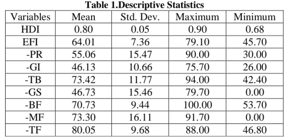
Table 1.Descriptive Statistics

Variables

Mean

Std. Dev.

Maximum

Minimum

HDI

0.80

0.05

0.90

0.68

EFI

64.01

7.36

79.10

45.70

-PR

55.06

15.47

90.00

30.00

-GI

46.13

10.66

75.70

26.00

-TB

73.42

11.77

94.00

42.40

-GS

46.73

15.46

79.70

0.00

-BF

70.73

9.44

100.00

53.70

-MF

73.30

16.11

91.70

0.00

-TF

80.05

9.68

88.00

46.80

Note: - reflects sub-indices of economic freedom index. PR: Property Rights, GR: Government Integrity, TB: Tax Burden, GS: Government Spending, BF: Business Freedom, MF: Monetary Freedom, TF: Trade Freedom.

Summary statistics of variables are expressed in Table 1. 7 sub-indices of economic freedom index out of 12 are considered, 3 of them are neglected due to lack of data, which are judicial effectiveness, fiscal health, and labour freedom; and investment freedom and financial freedom are excluded due to near singular matrix

The Impact of Economic Freedom on Human Development in European Transition Economies

____________________________________________________________

165

problem in bootstrap causality analysis. The correlation between HDI and EFI is 0.62. 𝐶𝐷𝐿𝑀1 = 𝑇 ∑ ∑ 𝜌𝑖𝑗2 𝑁−1 𝑗=1 𝑁 𝑖=1 (1)

Breush and Pagan (1980) create a test procedure for cross section dependency based on Lagrange Multiplier. 𝜌𝑖𝑗2 is the estimate of the cross sectional

correlation among residuals. Cross sectional dependence is tested for the null hypothesis of 𝐻0: 𝐶𝑜𝑣(𝜀𝑖𝑡, 𝜀𝑗𝑡) = 0 for 𝑖 = 𝑗, against the alternative hypothesis of

𝐻𝐴: 𝐶𝑜𝑣(𝜀𝑖𝑡, 𝜀𝑗𝑡) ≠ 0 for at least one couple of 𝑖 ≠ 𝑗 with a fixed 𝑁 and 𝑇 → ∞

under 𝜒2_{distribution based on (𝑁𝑥(𝑁 − 1)/2) degrees of freedom (Guloglu and}

Ivrendi, 2008). 𝐶𝐷𝐿𝑀2 = √ 1 𝑁(𝑁 − 1)∑ ∑ (𝑇𝜌𝑖𝑗 2 _{− 1)} 𝑁 𝑗=𝑖+1 𝑁−1 𝑖=1 ; 𝐶𝐷 = √ 2𝑇 𝑁(𝑁 − 1)∑ ∑ 𝜌𝑖𝑗 𝑁 𝑗=𝑖+1 𝑁−1 𝑖=1 (2)

Pesaran (2004) proposes a valid cross section dependency 𝐶𝐷𝐿𝑀2 testing

for size distortion, where 𝑁 → ∞ and 𝑇 → ∞. In accordance with this, he also develops a 𝐶𝐷 test for large 𝑁 and small 𝑇 situation for asymptotically standard normal distribution (Kar et al., 2011).

𝐿𝑀𝑎𝑑𝑗= √ 2 𝑁(𝑁 − 1)∑ ∑ (𝑇 − 𝑘)𝜌𝑖𝑗2𝜇𝑇𝑖𝑗 𝜈𝑇𝑖𝑗 𝑁 𝑗=𝑖+1 𝑁−1 𝑖=1 , 𝑤ℎ𝑒𝑟𝑒 𝐿𝑀𝑎𝑑𝑗~N(0,1) (3)

Pesaran et al. (2008) introduce a modified 𝐿𝑀 test for 𝑁 → ∞ and 𝑇 → ∞ due to the lack power situation of 𝐶𝐷 test, where mean pairwise correlations are zero (Menyah et al., 2014).

∆̃= √𝑁 (𝑁 −1_{𝑆̃ − 𝑘} √2𝑘 ) ; ∆̃𝑎𝑑𝑗= √𝑁 ( 𝑁−1_{𝑆̃ − 𝐸(𝑍̃} 𝑖𝑡) √𝑣𝑎𝑟(𝑍̃𝑖𝑡) ₎ (4)

Pesaran and Yamagata (2008) develop two testing, which are delta and delta-adjusted for the homogeneity of panel, whereas adjusted version is more appropriate for small samples. 𝐻0: 𝛽𝑖= 𝛽𝑗 is the null hypothesis of homogeneity

Mesut Alper Gezer

____________________________________________________________

One of the panel unit root test at the existence of cross section dependency is developed by Pesaran (2007), which take cross dependence of the series into consideration before standard unit root test procedure. This test enlarges the standard unit root procedure of ADF regressions with means of cross sections lagged levels and first differences of each cross section.

∆𝑦𝑖𝑡= 𝛼𝑖 + 𝛽𝑖𝑦𝑖,𝑡−1+ 𝑐𝑖𝑦̅𝑖,𝑡−1+ 𝑑𝑖∆𝑦̅𝑖+ 𝜀𝑖𝑡; 𝑓𝑜𝑟 𝑖 = 1,2, … , 𝑁; 𝑡 = 1,2, … , 𝑇 (5)

Cross section augmented regression model is expressed in equation 5, where 𝑦̅𝑖 is the cross section averages of each individual units.

𝑡𝑖(𝑁, 𝑇) =

∆𝑦_𝑖′𝑀̅𝑤𝑦𝑖,−1

𝜎̂𝑖(𝑦𝑖−1′ 𝑀̅𝑤𝑦𝑖,−1)1/2

(6) t ratio takes place in equation 6, where ∆𝑦𝑖 = (∆𝑦𝑖1, , … , ∆𝑦𝑖𝑇)′, 𝑦𝑖,−1 =

(𝑦_𝑖0, , … , 𝑦𝑖,𝑇−1) ′

, 𝑀̅𝑤= 𝐼𝑇− 𝑊̅ (𝑊̅′𝑊̅ )−1𝑊̅′, and 𝜎̂𝑖2=

∆𝑦_𝑖′𝑀𝑖,𝑤∆𝑦𝑖

𝑇−4 . The null

hypothesis of each cross section is 𝐻0𝑖: 𝛽𝑖=0, against the alternative hypothesis of

𝐻0𝑖: 𝛽𝑖<0 for the second generation panel unit root. Besides, CIPS statistics is also

introduced for the extreme values of each individual based on averages of each cross section as 𝐶𝐼𝑃𝑆 = 𝑁−1∑𝑁𝑖=1𝐶𝐴𝐷𝐹𝑖 for 𝑁 and 𝑇 tending to infinity.

Bai and Ng (2004) introduce PANIC test to clarify whether non-stationarity of a series stem from idiosyncratic part or common factor, or both of them in a second generation panel sense. Common factor based model is displayed in equation 7, where 𝐷𝑖𝑡 is polynomial trend function, 𝐹𝑡 is the common factor

vector, 𝑋𝑖𝑡 is the deterministic component, and 𝑒𝑖𝑡 is the idiosyncratic error term.

𝑋𝑖𝑡= 𝐷𝑖𝑡+ 𝜆𝑖′𝐹𝑡+ 𝑒𝑖𝑡 (7)

If the 𝐹𝑡 common factor is stationary in the model, which comes from

principal component, than 𝑒𝑖𝑡 idiosyncratic error term is the source of the unit root.

In accordance with this, they implement principal component to the first differenced equation of the model, and estimate loadings and common factors of each models by applying ADF regressions. They tested unit root for pooled model and group separately related with the homogeneity situation of the panel in terms of non-stationarity of null hypothesis.

Westerlund (2008) introduces Durbin-Hausman test for co-integration relationship in cross sectionally dependent series by using common factors. Common factor is determined according to principal components.

The Impact of Economic Freedom on Human Development in European Transition Economies

____________________________________________________________

167

Durbin-Hausman test statistics take place in equation 8, as pooled and group separately. While pooled statistics assumes homogeneity of panel, group statistics bases on heterogeneity. Null hypothesis leans on non-existence of co-integration as 𝐻0: ∅𝑖= 1 for all 𝑖 = 1, … , 𝑛 against alternative hypothesis of

co-integration 𝐻𝐴: ∅𝑖< 1 and 𝐻𝐴: ∅𝑖 = ∅ for all 𝑖 in pooled statistics. On the other

hand, 𝐻0: ∅𝑖 = 1 is tested against 𝐻𝐴: ∅𝑖 < 1 in group statistics for at least some 𝑖.

So rejection of null does not mean that all units are cointegrated in group statistics, but only for some. 𝑆̂𝑖= 𝑤̂𝑖2/𝜎̂𝑖4, 𝑆̂𝑛 = 𝑤̂𝑛2/(𝜎̂𝑛2)2, where 𝑤̂𝑖2 is the Kernel estimator.

∆𝑧𝑖𝑡= 𝜆𝑖′∆𝐹𝑡+ ∆𝑒𝑖𝑡, 𝐹𝑡 is the vector of common factors, and 𝑒̂𝑖𝑡= ∅𝑒̂𝑖𝑡−1+ 𝜀𝑖𝑡. 3.2. Estimators Methodology

Eberhardt and Bond (2009) put into forward two steps AMG method, which make consistent estimation for heterogeneous data under cross section correlation, including variable and factor non-stationarity.

𝑦𝑖𝑡= 𝛽𝑖′𝑥𝑖𝑡+ 𝑢𝑖𝑡 , 𝑢𝑖𝑡 = 𝛼𝑖+ 𝜆𝑖′𝑓𝑡+ 𝜀𝑖𝑡 (9)

𝑥𝑚𝑖𝑡= 𝛿𝑚𝑖′ 𝑔𝑚𝑡+ 𝜌1𝑚𝑖𝑓1𝑚𝑡+ ⋯ + 𝜌𝑛𝑚𝑖𝑓𝑛𝑚𝑡+ 𝜐𝑚𝑖𝑡 ; 𝑚 = 1, … , 𝑘 (10)

𝑓𝑡 = 𝜚′𝑓𝑡−1+ 𝜖𝑡 𝑎𝑛𝑑 𝑔𝑡 = 𝜅′𝑔𝑡−1+ 𝜖𝑡 (11)

Models are expressed in equations 9-11, 𝑥𝑖𝑡 is a vector of observable

covariables, 𝛼𝑖 is group specific fixed effect, 𝛽𝑖 are unknown random

coefficients, 𝜆𝑖 is country specific factor loadings, 𝑓𝑡 is a set of common factors, 𝑓𝑡

and 𝑔𝑡 are unobserved common factors’ linear functions, and 𝑓.𝑚𝑡 are subsets of 𝑓𝑡.

∆𝑦𝑖𝑡= 𝑏′∆𝑥𝑖𝑡+ ∑ 𝑐𝑡∆𝐷𝑡+ 𝑒𝑖𝑡 ; → 𝑐̂𝑡 ≡ 𝑢̂𝑡• ; 𝑆𝑡𝑎𝑔𝑒 (1) (12) 𝑇

𝑡=2

𝑦𝑖𝑡= 𝛼𝑖+ 𝑏𝑖′𝑥𝑖𝑡+ 𝑐𝑖𝑡 + 𝑑𝑖𝑢̂𝑡•+ 𝑒𝑖𝑡 ; 𝑆𝑡𝑎𝑔𝑒 (2) (13)

AMG estimator in two-stages is expressed in equation 12 and 13, where 𝑢̂𝑡•

are year dummy variables. In first stage, first difference regressions are taken into considerations to avoid bias estimates of nonstationary variables and un-observables. At second stage linear trend terms are added to reflect omitted idiosyncratic procedures. AMG estimators are attained according to means of individual country estimates, 𝑏̂𝐴𝑀𝐺 = 𝑁−1∑ 𝑏̂𝑖 𝑖.

Mesut Alper Gezer

____________________________________________________________

Pesaran (2006) suggests consistent and asymptotically normal coefficients estimates even in the case of correlations of unobserved common effects as well. He posits a multifactor residual model, and differentiates between individual specific effects and observed and unobserved common effects by introducing CCE estimator. The main idea of estimation process is to filtrates individual specific regressors by aggregates of cross section averages in a way of excluding unobserved common factor differential effects. It is seen that CCE is asymptotically unbiased estimator without any convergence restriction on 𝑁 and 𝑇. 𝑦𝑖𝑡= 𝛼𝑖′𝑑𝑡+ 𝛽𝑖′𝑥𝑖𝑡+ 𝑒𝑖𝑡 ; 𝑒𝑖𝑡= 𝛾𝑖′𝑓𝑡+ 𝜀𝑖𝑡 (14)

𝑥𝑖𝑡= 𝐴𝑖′𝑑𝑡+ Γ𝑖′𝑓𝑡+ 𝜐𝑖𝑡 (15)

Models of CCE estimation are expressed in equation 14 and 15, where 𝑑𝑡

is a vector of observed common effects, 𝑥𝑖𝑡 is a vector of observed individual

specific regressors, 𝑓𝑡 is the vector of unobserved common effects, 𝜀𝑖𝑡 is

idiosyncratic errors, 𝐴𝑖 and Γ𝑖 are loading factor matrices. Deterministic trends and

non-stationary roots are evaluated in 𝑥𝑖𝑡 and 𝑦𝑖𝑡 by letting at least one common

effect in 𝑑𝑡 and 𝑓𝑡, which have unit roots and/or deterministic trends.

𝑏̂𝑖= (𝑋𝑖′𝑀̅𝑤𝑋𝑖)−1𝑋𝑖′𝑀̅𝑤𝑦𝑖 (16)

Individual slope coefficients of CCE is demonstrated in equation 16, where 𝑀̅𝑤= 𝐼𝑇−𝐻̅𝑤(𝐻̅𝑤′𝐻̅𝑤)−1𝐻̅𝑤′, 𝐻̅𝑤= (𝐷, 𝑍̅𝑤) and 𝐷 and 𝑍̅𝑤 are matrices of

observations on 𝑑𝑡 and 𝑧̅𝑤𝑡. This estimator has been extended with CCEMG, which

is a simple mean of individual estimators, 𝑏̂𝑀𝐺 = 𝑁−1∑𝑁𝑖=1𝑏̂𝑖.

According to Driscoll and Kraay (1998) existence of cross section dependency causes inconsistent standard error estimates of coefficients. They propose a nonparametric correction for spatial dependence, which is similar to the nonparametric serial dependence of time series correction.

𝜃̂𝑇 = argmin {𝜃} ⌈ 1 𝑇∑ ℎ̃𝑡(𝜃) 𝑇 𝑡=1 ⌉ ′ 𝑆̃̂𝑇−1⌈ 1 𝑇∑ ℎ̃𝑡(𝜃) 𝑇 𝑡=1 ⌉ (17)

They use GMM covariance matrix estimator by hoarding 𝑅 orthogonality condition for each 𝑁, and 𝜃 is the parameter vector of this estimator. 𝑆̃𝑇 is a

consistent estimator of 𝑁𝑅𝑥𝑁𝑅 matrix, required for the variance estimation of GMM. So, non-parametric covariance matrix estimation causes robust standard error estimation against spatial dependence when 𝑇 is larger than 𝑁 dimension.

The Impact of Economic Freedom on Human Development in European Transition Economies

____________________________________________________________

169

Konya (2006) suggests bootstrap SUR panel simultaneous equation model to examine bivariate Granger causality relationship. This procedure has some advantages compared with other panel causality approaches. This process does not require pretesting of unit root and co-integration investigation due to bootstrap method’s extra information for panel dataset. It also reckons with cross section dependency, and the direction of causality is specified by Wald test with individual specific bootstrap critical values. The only imperative condition is to determine lag length before analysis. SUR models create better coefficient estimation than OLS models if simultaneous correlation exists in the system. Wald tests are applied to each individual and bootstrap statistics are obtained with ten thousands replicates.

ℎ𝑑𝑖1,𝑡= 𝛼1,1+ ∑ 𝛽1,1,𝑙 𝑙ℎ𝑑𝑖1 𝑙=1 ℎ𝑑𝑖1,𝑡−1+ ∑ 𝜃1,1,𝑙 𝑙𝑒𝑓𝑖1 𝑙=1 𝑒𝑓𝑖1,𝑡−1+ 𝜀1,1,𝑡 ℎ𝑑𝑖2,𝑡= 𝛼1,2+ ∑ 𝛽1,2,𝑙 𝑙ℎ𝑑𝑖1 𝑙=1 ℎ𝑑𝑖2,𝑡−1+ ∑ 𝜃1,2,𝑙 𝑙𝑒𝑓𝑖1 𝑙=1 𝑒𝑓𝑖2,𝑡−1+ 𝜀1,2,𝑡 (18) ⋮ ℎ𝑑𝑖𝑁,𝑡 = 𝛼1,𝑁+ ∑ 𝛽1,𝑁,𝑙 𝑙ℎ𝑑𝑖1 𝑙=1 ℎ𝑑𝑖𝑁,𝑡−1+ ∑ 𝜃1,𝑁,𝑙 𝑙𝑒𝑓𝑖1 𝑙=1 𝑒𝑓𝑖𝑁,𝑡−1+ 𝜀1,𝑁,𝑡 𝑎𝑛𝑑 𝑒𝑓𝑖1,𝑡= 𝛼2,1+ ∑ 𝛽2,1,𝑙 𝑙ℎ𝑑𝑖2 𝑙=1 ℎ𝑑𝑖1,𝑡−1+ ∑ 𝜃2,1,𝑙 𝑙𝑒𝑓𝑖2 𝑙=1 𝑒𝑓𝑖1,𝑡−1+ 𝜀2,1,𝑡 𝑒𝑓𝑖2,𝑡= 𝛼2,2+ ∑ 𝛽2,2,𝑙 𝑙ℎ𝑑𝑖2 𝑙=1 ℎ𝑑𝑖2,𝑡−1+ ∑ 𝜃2,2,𝑙 𝑙𝑒𝑓𝑖2 𝑙=1 𝑒𝑓𝑖2,𝑡−1+ 𝜀2,2,𝑡 (19) ⋮ 𝑒𝑓𝑖𝑁,𝑡= 𝛼2,𝑁+ ∑ 𝛽2,𝑁,𝑙 𝑙ℎ𝑑𝑖2 𝑙=1 ℎ𝑑𝑖𝑁,𝑡−1+ ∑ 𝜃2,𝑁,𝑙 𝑙𝑒𝑓𝑖2 𝑙=1 𝑒𝑓𝑖𝑁,𝑡−1+ 𝜀2,𝑁,𝑡

SUR model contemporaneous system dynamics are expressed in equations 18 and 19. 𝑙 is the predetermined lag length of the system, 𝑁 and 𝑇 are individual and time dimension respectively, and 𝜀1,1,𝑡 and 𝜀2,1,𝑡 are white noises and

Mesut Alper Gezer

____________________________________________________________

correlated for each cross sections. 1-4 lags are pre-assumed, and Schwartz information (𝑆𝐶𝑘 = 𝑙𝑛|𝑊| +

𝑁2𝑞

𝑇 ln (𝑇)) is predetermined before analysis. There is

unidirectional Granger causality running from EFI to HDI if in equation 18 not all 𝜃1,𝑖’s are zero, but all 𝛽2,𝑖’s are zero in equation 19. Moreover, there is

unidirectional causality running from HDI to EFI if all 𝜃1,𝑖’s are zero in equation

18, but not all 𝛽2,𝑖’s are zero in equation 19. Finally, there is bidirectional causality

between EFI and HDI if neither all 𝛽2,𝑖’s nor all 𝜃1,𝑖’s are zero, there is no Granger

causality between EFI and HDI, if all 𝛽2,𝑖’s and 𝜃1,𝑖’s are zero. 4. Empirical Findings

First of all, cross section contemporaneous correlation of each variable is discussed at Table 2.

Table 2.Findings of Cross Section Dependency

Tests

HDI

EFI

LM1

123.197***

98.119***

LM2

6.502***

4.111***

CD

-1.773***

-2.166***

LMadj

6.869***

2.387***

Note: *** indicates significance at 0.01 levels. 4 lag is determined for each evaluation. All calculations are done with Gauss 10.

It is seen that all variables has a trend in their series. So, all variables are tested under constant and trend assumption.

Table 3.Findings of Unit Root under Cross Section Dependency

Level

Tests

HDI

EFI

CIPS-stat

2.668

2.105

PANIC-Choi

-1.009

1.083

PANIC-Mw

15.304

29.181

First Difference

CIPS-stat

-2.948**

2.750*

PANIC-Choi

2.981***

3.762***

PANIC-Mw

41.776***

46.958***

Note: *, **, *** indicate significance at the 0.1, 0.05, and 0.01 levels, respectively. 4 lag is determined for each evaluation. All calculations are done with Gauss 10, and based on constant and trend together.

The Impact of Economic Freedom on Human Development in European Transition Economies

____________________________________________________________

171

Unit root findings are taken place in Table 3 according to Pesaran (2007) CADF test and Bai and Ng (2004) PANIC test. All variables have unit root at their level, and they get rid of from unit root in their first differences. So, variables are appropriate for cointegration investigation.

𝐻𝐷𝐼𝑖,𝑡 = 𝛼1+ 𝛽1𝐸𝐹𝐼𝑖,𝑡+ 𝜃1𝑡 + 𝜀𝑖,𝑡 ; 𝑀𝑜𝑑𝑒𝑙 1 (20)

𝐸𝐹𝐼𝑖,𝑡 = 𝛼2+ 𝛽2𝐻𝐷𝐼𝑖,𝑡+ 𝜃2𝑡 + 𝜀𝑖,𝑡 ; 𝑀𝑜𝑑𝑒𝑙 2 (21)

Models for cointegration relationship and estimator’s models are demonstrated in equation 20 and 21. Model 1 and Model 2 reflect bivariate reciprocal relationship between HDI and EFI.

Table 3.Cointegration and Homogeneity Findings

Tests

Model 1

Model 2

DH-panel

-0.502

-0.744

DH-group

-1.460*

-1.853**

Delta

4.233***

12.894***

Delta-adjusted

4.525***

13.784***

Note: *, **, *** indicate significance at the 0.1, 0.05, and 0.01 levels, respectively. 4 lag length and maximum common factor are determined for each evaluation under constant and trend. All calculations are done with Gauss 10.

While DH-panel deals with cointegration relationship under homogeneous pooled panel assumption, DH-group considers heterogeneity in panel data according to Westerlund (2008). Delta and Delta-adjusted examine homogeneity leaning on Pesaran and Yamagata (2008); in respect to this both of them reject homogeneity. Thus, DH-group findings are more proper for this panel structure, which reflect significant cointegration relationship in both models.

Table 4.Estimation Findings of Fixed Effect

Variables

Model 1

Economic Freedom

0.00114 (0.00028)***

Trend

0.00515 (0.00042)***

Constant

0.07795 (0.04193)*

Note: **, *** indicate significance at the 0.05, and 0.01 levels, respectively. All findings are attained with xtscc codes in Stata, and robust standard errors are reported in parenthesis.

Driscoll and Kraay (1998) fixed effect findings are displayed in Table 4, based on heteroscedasticity, autocorrelation, and cross section dependence

Mesut Alper Gezer

____________________________________________________________

consistent estimators. It is seen that economic freedom has positive and significant impact on human development.

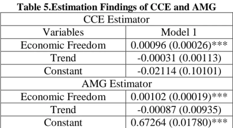
Table 5.Estimation Findings of CCE and AMG

CCE Estimator

Variables

Model 1

Economic Freedom

0.00096 (0.00026)***

Trend

-0.00031 (0.00113)

Constant

-0.02114 (0.10101)

AMG Estimator

Economic Freedom

0.00102 (0.00019)***

Trend

-0.00087 (0.00935)

Constant

0.67264 (0.01780)***

Note: **, *** indicate significance at the 0.05, and 0.01 levels, respectively. All findings are attained with xtmg codes in Stata, and robust standard errors are reported in parenthesis.

CCE and AMG findings support the results of Driscoll and Kraay (1998) fixed effect in Table 5. Economic freedom has positive and significant impact on human development. One unit increase in economic freedom approximately increases human development by 0.001 in the long run for bivariate relationship.

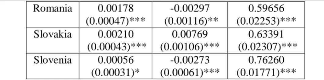
Table 6.Cross Section Findings of AMG

Countries

EFI

Trend

Constant

Bulgaria

0.00083

(0.00037)***

0.00501

(0.00060)***

0.65842

(0.01654)***

Croatia

0.00090

(0.00031)***

-0.00137

(0.054)**

0.67175

(0.01552)***

Czech R.

0.00035

(0.00042)

-0.00006

(0.00068)

0.74123

(0.02942)***

Estonia

0.00058

(0.00033)*

0.00005

(0.00062)

0.70119

(0.02308 )***

Hungary

0.00037

(0.00025)

-0.00069

(0.00037)*

0.72274

(0.01463)***

Latvia

0.00089

(0.00029)***

-0.00553

(0.00053)***

0.62936

(0.01797)***

Lithuania

0.00139

(0.00032)***

-0.00003

(0.00063)

0.63962

(0.01786)***

Poland

0.00161

(0.00036)***

0.00109

(0.00074)

0.66211

(0.02156)***

The Impact of Economic Freedom on Human Development in European Transition Economies

____________________________________________________________

173

Romania

0.00178

(0.00047)***

-0.00297

(0.00116)**

0.59656

(0.02253)***

Slovakia

0.00210

(0.00043)***

0.00769

(0.00106)***

0.63391

(0.02307)***

Slovenia

0.00056

(0.00031)*

-0.00273

(0.00061)***

0.76260

(0.01771)***

Note: *, **, *** indicate significance at the 0.1, 0.05, and 0.01 levels, respectively. All findings are attained with xtmg codes in Stata, and robust standard errors are reported in parenthesis.

Cross section findings of each country are displayed in Table 6, leaning on AMG estimator. All estimations are done with constant and trend models. All cross section estimators are found significant, excluding Hungary and Czech Republic. Economic freedom affects positively and significantly human development relatively more in Poland, Romania, and Slovakia in the long run.

4.1. Bootstrap Panel Causality Findings

Table 8.Panel Causality Findings I

H0: Economic Freedom does not cause Human Development

Countries

Wald

%1

%5

%10

Bulgaria

2.141

16.031

9.893

7.558

Croatia

0.825

16.300

8.441

5.671

Czech R.

2.832*

6.823

3.711

2.607

Estonia

3.910

14.329

8.397

5.863

Hungary

0.350

30.512

17.436

12.843

Latvia

0.168

14.097

7.076

4.849

Lithuania

0.645

20.095

9.709

6.355

Poland

0.191

24.306

14.146

10.457

Romania

4.480*

11.373

5.977

4.101

Slovakia

106.830***

71.361

47.720

38.479

Slovenia

0.294

12.608

6.453

4.377

Cross Section Dependency Findings of Causality Model

Tests

LM1

LM2

CD

LMadj

Statistics

911.736***

81.687***

30.063***

63.129***

Note: *, *** indicate significance at the 0.1, and 0.01 levels, respectively. Critical values are attained with 10.000 replications. All estimates are done with Gauss 10.

The strong and high correlation between HDI and EFI bring the question of causality between two. If countries have more economic freedom, this means more

Mesut Alper Gezer

____________________________________________________________

development. This increment in development may lead to more economic freedom further in the future (Gwartney et al., 1999). Bootstrap cross section causality findings running from economic freedom to human development takes place in Table 8. It is seen that there is significant findings of bootstrap Granger causality in Czech Republic, Romania, and Slovakia.

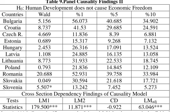
Table 9.Panel Causality Findings II

H0: Human Development does not cause Economic Freedom

Countries

Wald

%1

%5

%10

Bulgaria

5.156

56.073

40.685

34.902

Croatia

8.737

41.53

29.685

24.591

Czech R.

4.669

11.836

8.39

6.881

Estonia

0.689

15.317

9.268

7.132

Hungary

2.453

26.316

17.091

13.524

Latvia

1.108

24.885

16.135

13.058

Lithuania

8.773

31.933

22.533

18.745

Poland

0.793

21.836

14.845

12.109

Romania

20.688

52.931

39.758

33.984

Slovakia

0.049

30.594

21.618

17.721

Slovenia

5.507*

13.242

7.452

5.273

Cross Section Dependency Findings of Causality Model

Tests

LM1

LM2

CD

LMadj

Statistics

179.500***

11.871***

-0.922

63.046***

Note: *, *** indicate significance at the 0.1, and 0.01 levels, respectively. Critical values are attained with 10.000 replications. All estimates are done with Gauss 10.

Bootstrap cross section causality findings running from human development to economic freedom are displayed in Table 9. It is seen that there is significant unidirectional Granger Causality just in Slovenia. Meanwhile, whole panel causality findings also reveal that there is significant unidirectional bootstrap causality running from economic freedom to human development with 31.410* Panel Fisher value, whereas Panel Fisher value of causality findings from human development to economic freedom is 11.767 leaning on whole panel findings.

Bootstrap cross section significant findings running from economic freedom sub-indices to human development are taken place in Appendix 1. According to findings, there is evidence for unidirectional causality running from property rights (PR) to human development in Croatia, Latvia, and Romania. While there is unidirectional causality running from government integrity (GI) to HDI just in Poland, there is unidirectional causality from business freedom (BF) to HDI just in Estonia. Meanwhile, there is evidence of unidirectional causality from monetary

The Impact of Economic Freedom on Human Development in European Transition Economies

____________________________________________________________

175

freedom (MF) to HDI in Lithuania and Romania, whereas from trade freedom (TF) to HDI in Latvia, Lithuania, and Slovakia.

Bootstrap cross section significant findings running from human development to economic freedom sub-indices are taken place in Appendix 1 as well. According to findings, there is significant evidence running from HDI to GI in Slovakia, whereas from HDI to government spending (GS) in Slovenia. There is bidirectional causality between tax burden (TB) and HDI just in Slovenia. Moreover, there is unidirectional causality from HDI to TB in Bulgaria, Estonia, and Slovakia. There is unidirectional causality running from HDI to BF in Slovenia, Czech Republic, Lithuania; from HDI to MF in Czech Republic, and Latvia; and from HDI to TF just in Romania.

5. Conclusions

The objective of this study was to investigate the bivariate relationship between human development and economic freedom index for 11 European Transition Economies for the period spanning from 1996-2018. First of all, cross section dependency situation of units was examined, and unit root structure was analyzed by taking cross section dependency into consideration. It has been seen that there is unit root in level, and both are stationary in their first differences. At the second step, bivariate cointegration relationship has been brought out based on heterogeneity situation of the panel structure considering cross section dependency. After that, cointegration model has been estimated by CCE, AMG, and Driscoll and Kraay (1998) fixed effect estimators, which revealed similar findings as a whole. One unit increment in economic freedom approximately increases human development by 0.001. So, more freedom means more development for these countries in accordance with Goldsmith (1997) study. Besides, economic freedom affects positively and significantly human development relatively high in Poland, Romania, and Slovakia in the long run according to AMG cross section findings.

High correlation between human development and economic freedom brought the interrogation of causality relationship. It has been emerged that there is unidirectional causality running from economic freedom to human development based on Konya (2006) bootstrap panel causality in whole panel. According to cross section bootstrap Granger causality, there is evidence of one-way causality operating from economic freedom to human development in Czech Republic, Romania, and Slovakia, whilst there is evidence of one-way causality operating form human development to economic freedom just in Slovenia. As for the sub-indices of the economic freedom index, there is a one-way causality from private rights and monetary freedom to HDI in Romania, while in Slovakia there is a one-way causality from trade freedom to HDI and from government integrity to human development in Poland. Moreover, there is reciprocal two-way Granger causality between tax burden and human development in Slovenia. As a result, all findings imply that economic freedom is a crucial factor of development in CEE countries.

Mesut Alper Gezer

____________________________________________________________

REFERENCES

[1] Acikgoz, B., Amoah, A., Yılmazer, M. (2016), Economic Freedom and

Growth: A Panel Cointegration Approach. Panoeconomicus, 63(5):541-562;

[2] Bahtiyar, E., Karabacak, M. (2018), Economic Freedom and Human

Development: A Panel Causality Test on Selected Countries. The Seventh International Conference in Economics, 23-25 January,Lisbon: Econworld;

[3] Bai, J., Ng, S. (2004),A Panic Attack on Unit Roots and Cointegration.

Econometrica, 72(4): 1127-1177;

[4] Breush, T. S., Pagan, A. R. (1980),The Lagrange Multiplier Test and its

Application to Model Specification in Econometrics. The Review of Economic Studies, 27(2):19-32;

[5] Dawson, J. W. (2003),Causality in the Freedom-Growth Relationship.

European Journal of Political Economy, 19, 479-495;

[6] De Haan, J., Siermann, C.L.J. (1998),Further Evidence on the Relationship

between Economic Freedom and Economic Growth. Public Choice, 95,363-380;

[7] Driscoll, J. C., Kraay, A. C. (1998),Consistent Covariance Matrix Estimation

with Spatially Dependent Panel Data. Review of Economics and Statistics, 80(4):

549-560;

[8] Eberdhardt, M, Bond, S. (2009),Cross-Section Dependence in Nonstationary

Panel Models: A Novel Estimator. MPRA Working Paper 17692;

[9] Esposito, A., Zaleski, P. A. (1999),Economic Freedom and the Quality of

Life: An Empirical Analysis. Constitutional Political Economy, 10, 185-197;

[10] Farr, W.K., Lord, R.A., Wolfenbarger, J.L. (1998),Economic Freedom,

Political Freedom, and Economic Well-Being: A Causality Analysis. Cato Journal, 18(2): 247-262;

[11] Goldsmith, A. A. (2017),Economic Rights and Government in Developing

Countries: Cross-National Evidence on Growth and Development. Studies in Comparative International Development, 32(2): 29-44;

[12] Graafland, J. (2019),Contingencies in the Relationship between Economic

Freedom and Human Development: The Role of Generalized Trust. Journal of Institutional Economics, 1-16;

[13] Guloglu, B., Ivrendi, M. (2008),Output Fluctuations: Transitory or

Permanent? The Case of Latin America. Applied Economics Letters, 17(4):

381-386;

[14] Guney, T. (1997),Economic Freedom and Human Development. Hitit

University Journal of Social Science Institute, 10(2): 1109-1120;

[15] Gwartney, J. D., Lawson, R. A., Holcombe, R. G. (1999),Economic

Freedom and the Environment for Economic Growth. Journal of Institutional and Theoretical Economics, 155(4): 643-663;

[16] Heckelman, J.C. (2000),Economic Freedom and Economic Growth: A

The Impact of Economic Freedom on Human Development in European Transition Economies

____________________________________________________________

177

[17] Kar, M., Nazlıoğlu, Ş., Ağır, H. (2011),Financial Development and

Economic Growth Nexus in the MENA Countries: Bootstrap Panel Granger Causality Analysis. Economic Modelling, 28, 685-693;

[18] Menyah, K., Nazlıoğlu, Ş., Wolde-Rufael, Y. (2014),Financial

Development, Trade Openness and Economic Growth in African Countries: New Insights from a Panel Causality Approach. Economic Modelling, 37, 386-394;

[19] Konya, L. (2006),Exports and Growth: Granger Causality Analysis on

OECD Countries with a Panel Data Approach. Economic Modelling, 23,

978-992;

[20] Panahi, H., Assadzadeh, A., Rafaei, R. (2014),Economic Freedom and

Economic Growth in MENA Countries. Asian Economic and Financial Review,

4(1): 105-116;

[21] Pesaran, M. H. (2004),General Diagnostic Tests for Cross Section

Dependence in Panels. CESifo Working Paper 1229, IZA Discussion Paper 1240;

[22]Pesaran, M. H. (2006),Estimation and Inference in Large Heterogeneous

Panels with a Multifactor Error Structure. Econometrica, 74(4): 967-1012;

[23]Pesaran, M. H. (2007),A Simple Panel Unit Root Test in the Presence of

Cross-Section Dependence. Journal of Applied Econometrics, 22, 265-312;

[24]Pesaran, M. H., Ullah, A., Yamagata, T. (2008),A Bias-Adjusted LM Test of

Error Cross-Section Independence. Econometrics Journal, 11, 105-127;

[25]Pesaran, M. H., Yamagata, T. (2008),Testing Homogeneity in Large Panels.

Journal of Econometrics, 142, 50-93;

[26] Piatek, D., Szarzec, K., Pilc, M. (2013),Economic Freedom, Democracy and

Economic Growth: A Causal Investigation in Transition Countries. Post-Communist Economies, 25(3): 267-288;

[27] Ram, R. (2014),Measuring Economic Freedom: A Comparison Major

Sources. Applied Economics Letters, 21(12): 852-856;

[28] Sen, A. (1993),The Economics of Life and Death. Scientific American, 208(5): 40-47;

[29] Smith, A. (1776),An Inquiry into the Nature and Causes of the Wealth of

Nations. Cannan, E., Ed., London: Methuen, 1904, available at: https://oll.libertyfund.org/titles/237, last accessed 12.09.2019;

[30] The Heritage Foundation (2019),Index of Economic Freedom. Available at:

https://www.heritage.org/index/explore?view=by-region-country-year&u=637 119903210952288, last accessed 16.12.2019;

[31] UNDP (2010),The Real Wealth of Nations: Pathways to Human

Development. United Nations Development Programme Human Development Report, 20th _{Anniversary Edition;}

[32] UNDP (2019),Human Development Data 1990-2018. United Nations

Development Programme, available at: http://hdr.undp.org/en/data#, last accessed 27.01.2020;

[33] Westerlund, J. (2008),Panel Cointegration Tests of the Fisher Effect.

Mesut Alper Gezer

____________________________________________________________

[34] Wooldridge, J. M. (2013),Introductory Econometrics: A Modern Approach.

5th _{edition, Ohio: South-Western Cengage Learning.}

Appendix 1.Panel Causality Findings of Sub-indices of Economic Freedom

H0: Economic Freedom sub-indices does not cause Human Development

Causality

Countries

Wald

%1

%5

%10

PR->HDI

Croatia

35.110***

22.692

10.431

7.882

Latvia

9.840*

22.472

13.052

9.801

Romania

26.115*

45.015

30.414

23.921

GI->HDI

Poland

6.728**

8.230

5.718

4.686

TB->HDI

Slovenia

13.553***

10.855

5.257

3.576

BF->HDI

Estonia

24.270**

27.175

17.146

13.283

MF->HDI Lithuania

2.628**

2.970

1.639

1.143

Romania

83.998***

58.550

35.610

28.868

TF->HDI

Latvia

18.960*

30.333

19.946

16.380

Lithuania

29.475***

25.381

16.333

13.062

Slovakia

51.974*

83.206

55.187

44.940

H0: Human Development does not cause Economic Freedom sub-indices

HDI->GI

Slovakia

12.953***

8.944

4.735

3.192

HDI->TB

Bulgaria

11.560***

9.319

4.690

3.125

Estonia

12.564***

9.610

5.028

3.352

Slovakia

98.949***

72.657

48.046

38.815

Slovenia

20.975**

26.586

10.616

6.760

HDI->GS

Slovenia

18.094***

9.248

4.908

3.231

HDI->BF

Czech R.

22.371***

18.567

9.583

6.545

Lithuania

11.572**

13.032

6.061

3.926

HDI->MF

Czech R.

4.956*

12.203

6.441

4.378

Latvia

34.187***

28.722

18.090

13.991

HDI->TF

Romania

7.568*

15.944

7.771

5.060

Note: *, **, *** indicate significance at the 0.1, 0.05, and 0.01 levels, respectively. Critical values are attained with 10.000 replications. All estimates are done with Gauss 10. Non-significant findings are omitted to benefit from space, and available if demanded.