Assessment of the disaster recovery progress through mathematical modelling

Assessment of the Disaster Recovery Progress through

Mathematical Modelling

Natural disasters, especially major earthquakes, cause widespread devastation in the built environment. Hence, the major component of the recovery in its aftermath constitutes a chain of projects starting at different times, having different costs and durations. In this study, the post disaster recovery curve modelled through a mathematical approach taking into account these properties of the projects. The approach followed is based on the project S-curve concept that provides the opportunity to simulate the progress by outlining the project spending. Well-known mathematical functions are adapted to model the project spending and the handover processes. Monte Carlo simulation is performed to evaluate the general behavior of the recovery curve using the model developed. Weibull distribution is used to generate the model’s parameters. Results of the Monte Carlo simulation demonstrate that the recovery process exhibits an S-shape; the duration of initial portion and the slope of the bulk portion being significantly governed by the level of preparedness of the community.

Keywords: Disaster, recovery curve, mathematical modelling, S-curve, Monte Carlo

Simulation.

1. INTRODUCTION

Ever since, Bruneau et al (2003) introduced the model conceptualizing the resilience and the recovery of the societies following a major disaster, the model has found wide acceptance among both the academicians and administrators [1]. In their work, researchers presented a mathematical framework that paved road for the development of methodologies to measure the resilience also. Hence, possibly owing to the simplicity of the model, various approaches

Note:

- This paper has been received on October 22, 2018 and accepted for publication by the Editorial Board on April 22, 2019.

- Discussions on this paper will be accepted by xxxxxxx xx, xxxx.

 https://dx.doi.org/10.18400/tekderg.473099

1 MEF University, Civil Engineering Department, Istanbul, Turkey - dikmens@mef.edu.tr - https://orcid.org/0000-0002-4003-1368

2 Duzce University, Civil Engineering Department, Duzce, Turkey - rifatakbiyikli@duzce.edu.tr - https://orcid.org/0000-0003-1584-9384

3 Sakarya University, Institute of Natural Sciences, Sakarya, Turkey- murat.sonmez2@ogr.sakarya.edu.tr - https://orcid.org/0000-0003-2328-6817

to measure resilience have been developed and put in use (e.g. Cimellaro et al, 2010a&b) [2,3]. A comprehensive review of these studies can be found in the book on urban resilience by Cimellaro (2016) [4].

The model of Bruneau et al simply indicates that a sudden drop, namely a loss, in the functionality of the built environment and the society will take place in a disaster which will then be recovered in a period tt = tr-t0 through some path (Figure 1). In Figure 1, t0 and tr

correspond to the event date and the date total recovery is achieved, respectively. Likewise, in the same figure, Fd indicates the remaining functionality following the disaster.

Subsequently, the area above the recovery curve between times t0 and tr signifies the loss of

resilience, R, with respect to a specific disaster. Whereas, the area below the recovery curve is a measure of the resilience of the disaster hit community. Hence, the recovery curve is an important element in the resilience studies. Also, both the extent of loss, 100%-Fd and the

recovery period, tt, as well as the shape of the recovery curve are important parameters in

modeling and assessing the resilience and recovery of a community after a disaster.

Figure 1 - Conceptual representation of resilience (adapted from Bruneau et al 2003)[1]

Bruneau et al (2003) proposed that resilience has four components, namely technical, organizational, social and economic [1]. They involve many parameters of different difficulty levels to quantify. Researchers indicated that the first two components are related to the resilience of critical physical systems such as hospitals and lifelines. While, the last two components are more related to the affected community, such as housing. Thus, the term resilience covers a wide spectrum of topics ranging from human care to reconstruction and/or repair of the built environment. Generally, the major portion of the devastation by a disaster, regardless of its nature, is in the built environment. Therefore, to a great extent, full recovery, namely full functionality of the disaster hit community will require the revival of the built environment to the standards and scope prior to the disaster, including and of course but not limited to the satisfaction of housing needs.

Thus, another angle to look into the subject of functionality is the level of damage incurred in the built environment. This is especially true in the case of earthquakes. During a major earthquake, extensive damages and collapses in the built environment takes place [5]. Yet, it

is very difficult to estimate the extents and composition of the structures and facilities damaged before the disaster [6]. While some structures will become functional with minor or major repairs, others may be in a condition beyond repair. Furthermore, the damaged structure can be a structure with low replacement cost and short implementation time or a facility with high replacement cost and duration [7]. The common point among all these efforts is that, they all are projects of different cost magnitude and duration. Hence, the major component of the recovery from a disaster will constitute a chain of projects starting at different times, having different costs and different durations. In this respect, if the full recovery of the damaged inventory is considered as a “project”, the projects in the chain can be termed as “sub-projects”. In other words, all sub-projects will have the objective to make good some function lost in the built environment during the disaster. Therefore, the shape of the recovery curve will be analogous to the progress curve of the overall recovery project, i.e. the chain of sub-projects.

Cimellaro et al (2006) suggested that the recovery curve can be represented by three different forms, namely linear, exponential and trigonometric [8]. In their work, the linear recovery is attributed to the recovery of an average prepared community. They also stated that if the community is well prepared the recovery curve will take the form of the exponential (convex) curve, while the recovery of an unprepared community will follow a trigonometric (concave) path (Figure 2).

Figure 2 - Recovery functions (adapted after Cimellaro et al (2006, 2010) [2,3,8])

In project management, especially in construction project management, the cash flow of projects, in general, follow a curve known as S-curve. In other words, it can be stated that an S-curve is a mathematical form to represent the cash flow of a project (Kenley, 2005) [9]. By analyzing the S-curves, the management team can identify visually if a project is on time or delayed and in or over budget. In this respect, the S-curve constitutes one of the basic concepts in project management. The use of estimated S-curves is a common practice among the owners, contractors and administrations in project planning, especially for forecasting the

cash flow. With this token, assuming that the recovery process in the aftermath of a disaster consists of a number of small projects, i.e. sub-projects, one can construct the project spending curve by combining the S-curves and subsequently the functionality contribution of the sub-projects, as named earlier.

The objective of this study is the investigation and assessment of the trend of the disaster recovery curve using a mathematical model based on the project curve. The form of the S-curve is selected in accordance with the earlier S-S-curve models developed. Then a Monte Carlo simulation type analysis is performed to observe the general behavior of the recovery curve based on the hypothesized model.

2. THE MATHEMATICAL MODEL

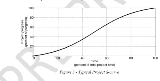
Researchers analyzing past data have determined that cumulative cash flows during the course of a project, especially in construction projects, display an S-shaped curve. A typical S-curve of a construction project starts gradually with a small slope basically covering the mobilization and initial works, such as excavation (Figure 3). Then the curve has a higher slope when the bulk of the production takes place, such as structural works, interior finishes and the façade works. Finally, the rate of increase of the curve slows down nearing the end of the project when most of the efforts at site are devoted to finalizing various cost items and the commissioning activities of the facility.

Figure 3 - Typical Project S-curve

Although, this shape generally applies to most of the projects, it should be noted that some variations can exist having impact on the shape of the curve, namely the cumulative cash flow curve at completion of a project may not be as smooth as the one shown in Figure 3. However, historical data prove that the spending at most of the projects closely follows a trend signified by the S-curve. In this respect, analyzing historical data researchers have proposed various mathematical expressions for the S-curve (Hudson & Maunick, 1974; Peer, 1982; Kenley & Wilson, 1986; Miskawi, 1989; Khoshrowshahi, 1991; Bousbaine and Elhag, 1999) [10,11,12,13,14,15,16]. Amongst various curves proposed, a well-known curve is the one developed by The Department of Health and Security of the United Kingdom (DHSS)

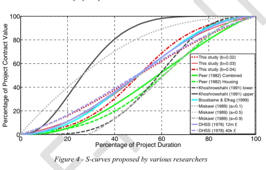
based on Hudson’s studies on the subject (Hudson, 1978) [17]. A detailed treatment of the S-curve, including comparison of generic S-curves derived by various researchers, is given in the book on construction financing by Kenley (2005) [9]. A graphical summary of some the S-curves proposed by various researchers are given in Figure 4. Obviously, some differences exist between the proposed curves due to factors such as the composition and characteristics of the data set used, business culture of the country data collected. For instance, the DHSS curves are based on the construction of health care facilities with total value of about 12m £ at the time of the study. On the other hand, Miskawi and Khoshrowshahi curves represent some upper and lower bounds, which require selection of a parameter particular to the method for the determination of a project specific curve.

Figure 4 - S-curves proposed by various researchers

For the purposes of this study, a generic S-curve, assumed to be valid for all projects, namely the sub-projects, as defined earlier, is used. This curve is mathematically represented by the so-called logistic function in the following form,

𝐸 (𝑡) = (1)

Where a and b are constants. Constants a and b determine the rate of increase and the shape of the curve. The limiting value Csp is the total expenditure for the sub-project. If b is positive,

as in our case, the curve will demonstrate an increasing trend. Time passed from the incision of the project, evaluated as the percentage of the total duration of the sub-project, appears as t in the equation. If the abscissa values, expenditure Esp(t), are normalized with respect to

total sub-project expenditure, Csp and the horizontal axes values, time t, normalized with

respect to the total sub-project duration, we obtain a normalized generic S-curve in terms of percentages of progress and total project duration. The logistic curve has a single inflection point. The curve has two equal regions of opposite concavity with respect to this point. The

0 20 40 60 80 100 0 20 40 60 80 100

Percentage of Project Duration

P ercentage of P rojec t C ontract V alue This study (b=0.02) This study (b=0.03) This study (b=0.04) Peer (1982) Combined Peer (1982) Housing Khoshrowshahi (1991) lower Khoshrowshahi (1991) upper Bousbaine & Elhag (1999) Miskawi (1989) (a=0.1) Miskawi (1989) (a=0.5) Miskawi (1989) (a=0.9) DHSS (1978) 12m £ DHSS (1978) 40k £

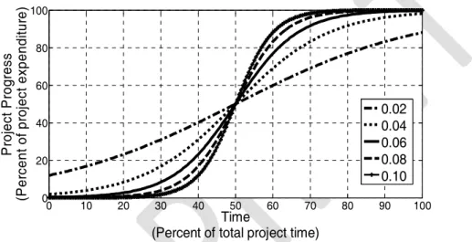
coordinates of the inflection point are , . Further detailed information about the properties of the logistic curve can be found in books on calculus and differential equations. If variable a is equal to unity, than the point of inflection of the S-curve will be at zero time and at half the expenditure of the sub-project conserving the concave symmetry around the abscissa. Hence, the S-curve calculated in this fashion is then shifted in the positive direction by half the duration of the sub-project. The S-curves for different combination of values of variable b and a is constant and equals to unity are given in Figure 5.

Figure 5 - Normalized generic project S-Curve

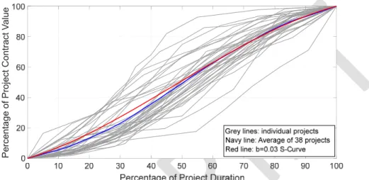
The curves for b=>0.06 are asymptotic with negligible values at 0 and 100% points in time, while for lesser values of b curves exhibit some finite value at these ends. Namely, these curves are asymptotic near the 0 and 100% and above. On the other hand, the curves with b=>0.08 have sustained negligible progress value for time percentages less than 30% and higher than 70%, which is not usual for the projects rolling normally. However, the curves in real life are not asymptotic at the beginning and at the end of a project as demonstrated in Figure 4. Hence, b value for the generic S-curve needs to be =<0.04; the abscissa values of the curves b=<0.04 can be adjusted by prorating to 100% expenditure. The S-curves adjusted in this fashion with b=0.02, 0.03 and 0.04 are demonstrated in Figure 4 together with the curves proposed by others. The curve with b=0.03 matches very closely with the DHSS curve for 12m £ projects as well as exhibits an average trend with respect to the other curves. Furthermore, cash flow data of 38 different disaster recovery projects realized in Turkey were analyzed. These projects were constructed by The Housing Development Administration of Turkey between 2007 and 2014. Each individual project consists of a number of apartment buildings, social and technical infrastructure as well as landscaping. The average completion cost of the projects were about 20.0 mil USD. It is also important to note that groups of several projects were constructed for the recovery of different earthquakes. The percent of realization vs percent of time graphs of these projects are shown in Figure 6 together with

0 10 20 30 40 50 60 70 80 90 100 0 20 40 60 80 100 Time

(Percent of total project time)

P roj ec t P rogr ess (P er ce nt of pr oj ect expendi tu re ) 0.02 0.04 0.06 0.08 0.10

their average. The generic S-curve with b=0.03 is also included in this figure. The close match of the b=0.03 curve with the average percent of realization vs percent of time of the recovery projects is remarkable. Therefore, considering the closeness of match with the DHSS curve and the average curve of the 38 earthquake recovery projects, b=0.03 was set to be used in generic S-curve definition.

Figure 6 - Comparison of the b=0.03 S-Curve with data from projects realized in Turkey

The project progress curve or the recovery curve will be the summation of the n number of sub-projects necessary for full recovery. This can be mathematically represented as,

𝐸(𝑡) = ∑ 𝐸 (𝑡) = ∑ (2)

As shown in the equation, each sub-project will have different values for variables a, b and Csp signified by subscript n. Furthermore, each sub-project will have a different start time

and duration that will be reflected by variable for time, t.

For the simulation purposes, the sub-project costs 𝐶 can be randomly determined using an appropriate distribution function. Similarly, one can determine the start time and the duration of each sub-project randomly. Subsequently the function E(t) can be evaluated using a=1 and b=0.03 (as determined earlier), which then can be shifted to the interval between t to t + sub-project duration.

The achieved functionality rate of each sub-project will not be the same also. Based on their contracts, while in some projects the commissioning of the project is at the end of the project duration, in some projects partial handovers to the owner can take place during the course of the project. Hence, the expenditure curve obtained by Eq. 2 will not be the same as the progress of functionality. This can be achieved by multiplying Eq. 1 of each sub-project by a function, such as an exponential function of the following form,

𝐻(𝑡) = 𝑒 (3) Percentage of P roject C ontract V alue

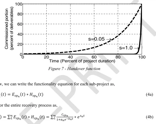
where, s is a constant that determines the rate of increase, in turn the shape of the curve. t is time as before. The handover curves for s=0.05 and s=1.0 is shown in Figure 7. The s=1.0 curve can be considered for the handover at the end of the project as in the case of single buildings. Similarly, s=0.05 curve can be considered as the gradual handover almost from the start. The rate in the analysis will be selected between these values randomly.

Figure 7 - Handover function

Now, we can write the functionality equation for each sub-project as,

𝐹 (𝑡) = 𝐸 (𝑡) ∗ 𝐻 (𝑡) (4a)

or for the entire recovery process as,

𝐹(𝑡) = ∑ 𝐸 (𝑡) ∗ 𝐻 (𝑡) = ∑ ∗ 𝑒 (4b)

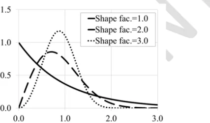
As noted above, for the determination of the variables, one needs to decide on the type of distribution, which in this case Weibull distribution is used. The Weibull distribution is a flexible distribution model that can be characterized by two parameters, namely shape and scale factors, to display different probability distribution functions (Figure 8). When the shape factors approaches to 1.0, the probability density curve takes the form of an exponentially decaying curve. While on the other when the shape factor is greater than 1.0, the probability density function will be approaching towards a normal distribution with the mean depending upon the scale factor.

One also needs to set the rules about the ranges of the variables so that they reasonably replicate the real life cases. Thus, it is essential to observe the following limiting conditions regarding the sub-project S-curves,

 The total value of the sub-projects cannot exceed the total expenditure for recovery as given in Eq. 2

 The duration of each sub-project cannot exceed the overall recovery period,

0 20 40 60 80 100 0 20 40 60 80 100 s=1.0 

Time (Percent of project duration)

C om m is si on ed por tion ( per ce nt of del iv er abl es ) s=0.05 

 The completion date of any sub-project cannot be after the full recovery date  The start date of each individual sub-project cannot be earlier than the disaster date Considering these limitations, two sample cases were evaluated assuming that 250 and 1000 sub-projects are needed for full recovery. Furthermore, for each case Weibull distribution with shape factors 1.0 and 2.0 were used to determine the sub-project cost, time of start of each sub-project and the duration of the sub-project. The resulting curves are displayed in Figure 9. Another constraint used in the analysis is that the sub-projects will have durations of 3.0-90.0% of the total recovery period. The 3% duration will correspond to approximately 1-2 months for recovery periods 3-5 years, which is a reasonable period when repair projects are considered.

Figure 8 - Probability density curves for Weibull distribution (Scale factor =1.0)

Figure 9 - Expenditure (left pane) and recovered lost functionality (right pane) curves

Expenditure (%) Rec o ve red lost functionality (%)

3. MONTE CARLO SIMULATION AND DISCUSSION OF RESULTS

A Monte Carlo simulation study is conducted to observe the behavior of the recovery curve proposed by Eq. 4 with respect to the variations in the distribution of cost, duration and the start time of the sub-projects. Monte Carlo simulation is a computer based mathematical technique. It allows the user to account for the variability of the factors in the process. Hence the process involves a variation analysis by constructing models of possible results through the substitution of a range of values for any variable or factor that has inherent uncertainty. Then each time using a different set of random values from the probability functions results are calculated for a large number of times.

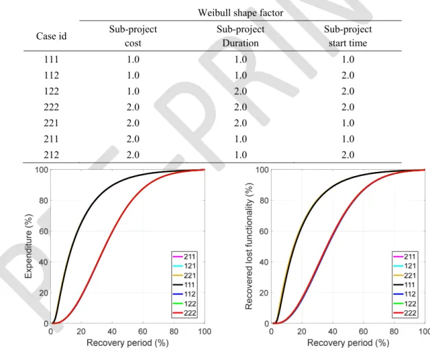
Table 1 - Case combinations considering Weibull shape factors for cost, duration and start time of the sub-projects

Weibull shape factor Case id Sub-project cost Sub-project Duration Sub-project start time 111 1.0 1.0 1.0 112 1.0 1.0 2.0 122 1.0 2.0 2.0 222 2.0 2.0 2.0 221 2.0 2.0 1.0 211 2.0 1.0 1.0 212 2.0 1.0 2.0

Figure 10 - Progress (left pane) and Functionality (right pane) curves (scale factor for sub-project duration taken as 1.0)

Ex penditure (%) Recov ered lost functionality (%)

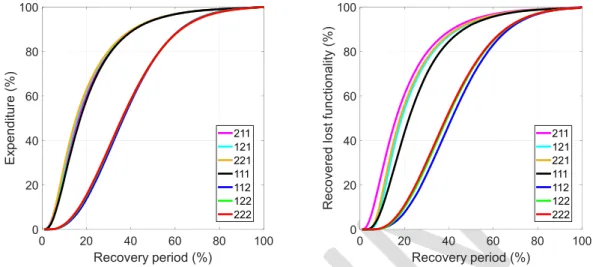
Figure 11 - Progress (left pane) and Functionality (right pane) curves (scale factor for sub-project duration taken as 5.0)

For the selection of the sub-project monetary sizes, two different random distribution schemes by varying the shape factors were employed. The combinations based on these parameters are determined and tabulated (Table 1). On the other hand, the shape factor was only varied for the sub-project duration, namely by using 1.0 in the first analysis set and by using 5.0 in the second set. For all cases, the simulations were made for 2500 trials and the mean curves calculated for the two different shape factors of the sub-project duration (Figures 10 and 11).

The observations and findings from the results of the simulations can be summarized as follows,

 All simulation cases, fourteen altogether, using different statistical distributions of sub-project values yielded very similar shaped average recovered functionality curves with respect to the recovery period. They all yielded S-shaped curves, as would be expected. Earlier results, either analytically derived or recorded from actual case studies, reported in a number of valuable studies support this trend of the recovery period (e.g. Ouyang and Wang, 2015; Zobel, 2013; Porter, 2016) [18,19,20]. However, a variation in the spread of curves exists.

 The curves seem to accumulate in two groups regardless the scale factor (Figures 10 and 11). The common factor in each group is the shape factor of the sub-project value. The group with the shape factor=1.0 for the subproject values displays a faster recovery curve as compared to the other group with shape factor=2.0 for the sub-project values. The shape factor of the sub-project duration and the start time seem not to have a significant effect on the outcome. This is indeed reasonable and an expected outcome. Because shape factor=1.0 for the sub-project values reflect that majority of the sub-projects will have relatively low budget activities, i.e. repair or small projects. Whereas the shape

0 20 40 60 80 100 Recovery period (%) 0 20 40 60 80 100 Ex penditure (%) 211121 221 111 112 122 222 0 20 40 60 80 100 Recovery period (%) 0 20 40 60 80 100

Recovered lost functionality

(%) 211 121 221 111 112 122 222

factor=2.0 can be deemed to represent less number of repair works and higher number higher budget sub-projects.

 Furthermore, to investigate the possible impact of number of sub-projects two additional simulations were made using 25 and 500 sub-projects for the cases 111 and 222 with shape factor=2.0. Both the expenditure and the recovered lost functionality curves had coincided with the previous simulations with 250 sub-projects.

 The build-up of recovery of lost functionality curve starts slowly and grows faster in the later stages. It is important to note that the generic recovery curve includes the impact of the sub-projects only and excludes the preparatory works, such as planning and contracting works. In that respect, it should be expected that the initial slow period will be extended accordingly. However, this extension will be closely related to the preparedness of the community to deal with the processes after the disaster.

 Towards the end of the recovery period, the curves display a slower progress. That is basically due to the commissioning and handover processes of the sub-projects. In this respect, it can be hypothesized that at the curvature point, around 90-95% recovery, “substantial recovery” is achieved.

 Hence, the S-curves can be split into three parts considering the curvature points, concave and convex of these curves. The three parts can be identified as the initial period, the main recovery period and the substantial recovery period.

 Assuming that at the substantial recovery period stage, the community has returned back to almost full functionality, the main governing factors of the recovery curve are the duration of the initial period and the slope of the main recovery period. Based on the findings above, both the length of the initial period and the main recovery period will be mainly governed by the monetary sizes of the sub-projects. Hence, for instance at places where the risk of a major earthquake exists, it will be appropriate to strengthen first the structures within the modal monetary value group of the risky stock in the built environment. Such a strategy will increase the resilience of the community and shorten the overall recovery period.

4. CONCLUSION

The recovery curve of a community, in the aftermath of a destructive event such as a major earthquake is evaluated through mathematical modelling. The mathematical model used is based on the project S-curve concept that is widely accepted and widely utilized in the project management community, especially in the construction sector.

Results of the Monte Carlo simulation demonstrate that the recovery process exhibits an S-shape, the duration of initial portion and the slope of the bulk portion being significantly governed by the level of preparedness of the community. Namely, the higher the level of preparedness, the shorter will be the recovery process. Hence, a viable strategy in increasing the pace of the recovery, namely resilience, to be considered would be the strengthening of the group of structures (including infrastructure) that are in the modal monetary value group among the risky sub-projects. Thus, by reducing the damage of these structures in the event of a major disaster, the recovery process can be significantly expedited. Furthermore, the recovery of the community will start earlier as compared to less prepared cases.

Symbols

a, b = constants

Csp = Total expenditure (cost) for the sub-project

E(t) = Expenditure function of project Esp(t) = Expenditure function of sub-project

Fd = Remaining functionality following disaster

H(t) = Handover function of sub-project R = lost resilience

S = t = Time t0 = Event date

tr = Date total recovery achieved

tt = Total duration of recovery

Acknowledgements

The authors wish to express their gratitude to the Istanbul office of Housing Development Administration of Turkey (TOKI) and the consulting and construction supervision companies, who preferred to remain anonymous, for providing the data of the post disaster projects in Turkey.

References

[1] Bruneau, M., Chang, S., Eguchi, R. Lee, G., O’Rourke, T., Reinhorn, A., Shinozuka,M., Tierney, K., Wallace, W., von Winterfelt, D., (2003). “A framework to Quantitatively Assess and Enhance the Seismic Resilience of Communities”, EERI Spectra Journal, 19, (4), 733-752

[2] Cimellaro, G.P., Reinhorn, A.M., Bruneau, M. (2010a) “Seismic resilience of a hospital system” Structure and Infrastructure Engineering, Vol. 6, Nos. 1–2, February–April 2010, 127–144

[3] Cimellaro, G.P., Reinhorn, A.M., Bruneau, M. (2010b) “Framework for analytical quantification of disaster resilience” Engineering Structures 32 (2010) 3639–3649 [4] Cimellaro, G.P. (2016) “Urban Resilience for Emergency Response and Recovery

Fundamental Concepts and Applications” Springer International Publishing Switzerland

[5] Güler, H.G, Sözdinler, C.Ö., Arikawa, T., Yalçıner, A.C. (2018) “Tsunami Afeti Sonrası Yapısal ve Yapısal Olmayan Önlemler ve Farkındalık Çalışmaları: Japonya Örneği”, Teknik Dergi, 8605-8629

[6] Şengöz, A., Sucuoğlu, H., (2009) “2007 Deprem Yönetmeliğinde Yer Alan “Mevcut Binaların Değerlendirilmesi” Yöntemlerinin Artıları ve Eksileri”, Teknik Dergi, 4609-4633

[7] Yanmaz, Ö., Luş, H., (2005) “Yapı Güçlendirme Yöntemlerinin Fayda-Maliyet Analizi”, Teknik Dergi, 3497-3522

[8] Cimellaro, G.P., Reinhorn, A.M., Bruneau, M. (2006) “Quantification of Seismic Resilience”, Proceedings of the 8th U.S. National Conference on Earthquake Engineering, April 18-22, San Francisco, California, USA

[9] Kenley, R. (2005), Financing Construction – Cash Flows and Cash Farming, Taylor and Francis e-Library, ISBN 0-203-46739-6.

[10] Hudson, K. W. and Maunick, J. (1974). Capital expenditure forecasting on health building schemes, or a proposed method of expenditure forecast. Research report, Surveying Division, Research Section, Department of Health and Social Security, UK. [11] Hudson, K. W. and Maunick, J. (1974). Capital expenditure forecasting on health

building schemes, or a proposed method of expenditure forecast. Research report, [12] Peer, S. (1982). ‘Application of cost-flow forecasting models’. Journal of the

Construction Division, ASCE, Proc. Paper 17128, 108 (CO2): 226–32.

[13] Kenley, R., and Wilson, O. D. (1986) “A construction project cash flow model-An idiographic approach.” Construction Management and Economics, 4(3), 213–232. [14] Miskawi, Z. (1989) “An S-curve equation for project control.” Construction

Management and Economics, 7(2), 115–124.

[15] Khosrowshahi, F. (1991) ‘Simulation of expenditure patterns of construction projects Construction Management and Economics 9(2): 113–132.

[16] Boussabaine, A. H. and Elhag, T. (1999). ‘Applying fuzzy techniques to cash flow analysis’. Construction Management and Economics 17: 745–755.

[17] Hudson, K. W. (1978). ‘DHSS expenditure forecasting method’. Chartered Surveyor— Building and Quantity Surveying Quarterly 5: 42–45.

[18] Ouyang, M., Wang, Z. (2015) “Resilience assessment of interdependent infrastructure systems: With a focus on joint restoration modeling and analysis”, Reliability Engineering and System Safety, 141(2015)74–82, doi.org/10.1016/j.ress.2015.03.011 [19] Zobel, C.W., (2013) “Analytically comparing disaster recovery following the 2012

derecho”, Proceedings of the 10th International ISCRAM Conference – Baden-Baden, Germany, May 2013 T. Comes, F. Fiedrich, S. Fortier, J. Geldermann and T. Müller, eds.

[20] Porter, K. (2016) “Damage and Restoration of Water Supply Systems in an Earthquake Sequence”, Structural Engineering and Structural Mechanics Program, Department of Civil Environmental and Architectural Engineering, University of Colorado, SESM 16-02, July 2016.