Short-term load forecasting by using artificial neural networks

(1)

T.C.

BAHÇEŞEHİR ÜNİVERSİTESİ

SHORT-TERM LOAD FORECASTING

BY USING ARTIFICIAL NEURAL NETWORKS

Master’s Thesis

USMAN NAJEEB KHAN

(2)

(3)

THE REPUBLIC OF TURKEY

BAHCESEHIR UNIVERSITY

NATURAL AND APPLIED

SCIENCES

ELECTRICAL AND ELECTRONICS

ENGINEERING

SHORT-TERM LOAD FORECASTING

BY USING ARTIFICIAL NEURAL NETWORKS

Master’s Thesis

USMAN NAJEEB KHAN

Supervisor: ASSIST. PROF. CAVİT FATİH KÜÇÜKTEZCAN

(4)

THE REPUBLIC OF TURKEY BAHCESEHIR UNIVERSITY

THE GRADUATE SCHOOL OF NATURAL AND APPLIED SCIENCES

ELECTRICAL AND ELECTRONICS ENGINEERING

Name of the thesis: Short-Term Load Forecasting by Using Artificial Neural Networks

Name/Last Name of the Student: Usman Najeeb KHAN Date of the Defense of Thesis: 25 May 2018

The thesis has been approved by the Graduate School of Natural and Applied Sciences.

Assist. Prof. Yücel Batu SALMAN Graduate School Director

Signature

I certify that this thesis meets all the requirements as a thesis for the degree of Master of Natural and Applied Sciences.

Assist. Prof. Cavit Fatih KÜÇÜKTEZCAN Program Coordinator

Signature

This is to certify that we have read this thesis and we find it fully adequate in scope, quality and content, as a thesis for the degree of Master of Science.

Examining Comittee Members Signature____

Thesis Supervisor ---

Assist. Prof. Cavit Fatih KÜÇÜKTEZCAN

Member ---

Prof. Dr. Ayşen DEMİRÖREN

Member ---

(5)

ACKNOWLEDGEMENTS

Mainly, I am thankful to God for encouraging me to carry out with this bit of work and especially the way He helped me through many difficulties that came at the primary of my investigations. I sincerely thank my Supervisor Dr. Cavit Fatih Küçüktezcan for his magnificent help and direction during the whole time of the research. I am also thankful for the input I got from my teachers/staff individuals at the Bahcesehir University for their enormous dedications toward the fulfilment of this research work. I also acknowledge the help from chose specialists, authority and the staff individuals who gave their opportunity and vitality to partake in the meeting procedure. I salute them, particularly the foundation where this meeting was done, and in addition the on-screen character respondents who have influenced this exploration to meet the reality finally. I am also thankful to Dr. Gürkan Soykan for his guidance and motivation when I was through a hard time of the research. In addition, I also want to thank the Load Dispatch Centre (LDC) staff of Faisalabad Electric Supply Corporation (FESCO) for providing the electric demand load data.

This research could not have been completed if it had not been with the help and trust of the previously mentioned recognized personalities who bestowed their opportunity and vitality to give me all the fundamental data and guidance required for the task to meet the reality. I acknowledge and salute them just for their several agreements for this research work which will profit numerous in the groups and the world on the loose.

(6)

ABSTRACT

SHORT-TERM LOAD FORECASTİNG BY USİNG ARTİFİFİCAL NEURAL NETWORKS

Usman Najeeb Khan

Electrical and Electronics Engineering Asst. Prof. Dr. Cavit Fatih Küçüktezcan

May 2018, 53 pages

Load forecasting is a vital component for power systems. For any electric power organization, it is their main role to provide electric energy in an economical and secured manner maintaining the quality. In power systems, electric load forecasting is a very essential issue and has been studied widely so that to attain more precise load forecasting results. Since in power systems the next day's power generation must be scheduled every day, day-ahead short-term load forecasting (STLF) is an important daily task for power companies. The short-term load forecast represents the electric load forecast for a time span of few hours to a several days.

This thesis uses the method of Artificial Neural Networks (ANN) to create a STLF model for Faisalabad Electric Supply Cooperation (FESCO). FESCO can be described as an institutional/industrial-type electric load. The ANN is a mathematical/computational tool that mimics the way human brain processes information. Several types of ANNs are revealed in this research, among them Feed-Forward (FF) neural networks have been used to create a STLF model.

Two different methods ReliefF and Correlation analysis are presented and used for the selection of important input variables which will be used as inputs of ANN. The inputs given to the ANN are historical electric load and average air temperature data.

Correlation method provides better results for the selection of input variables rather than the ReliefF method. The ANN uses the historical electric load and weather data as an input and provides a forecasted electric load at its output. Average air temperature data is used in this research in order to achieve better short-term load forecasting results.

Furthermost ANNs in the literature are used to forecast day ahead electric load for a transmission-level system with resulting load forecast errors ranging from nearly 0.1% to 2.3%. This research indicates that an ANN can be used to forecast the smaller, more disordered load profile of an institutional/industrial-type power system and results in a similar forecast error range. In addition, the in-service constraints of the FESCO electric load will be investigated along with the weather profiles for the site.

(7)

Through detailed performance evaluations, this research demonstrate that the presented forecasting method is capable of predicting the day ahead electric load accurately.

Keywords: Short-Term Load Forecast, Artificial Neural Network, Multi-Layer Perceptron, Feed-Forward Neural Network, Back-Propagation Algorithm

(8)

ÖZET

SHORT-TERM LOAD FORECASTİNG BY USİNG ARTİFİFİCAL NEURAL NETWORKS

Usman Najeeb Khan

Elektrik ve Elektronik Mühendisliği Asst. Prof. Dr. Cavit Fatih Küçüktezcan

Mayıs 2018, 53 sayfa

Yük tahmini, güç sistemleri için hayati bir bileşendir. Elektrik enerjisinin ekonomik ve güvenli bir şekilde tüketiciye sağlanması elektrik güç sistemi kurumlarının temel rolüdür. Güç sistemleri için önemli bir konu olan elektriksel yük tahminin daha yüksek başarımla yapılabilmasi amacıyla çalışılmaktadır. Güç sistemlerinde, ertesi güne ait güç üretiminin şimdiden planlanması gerektiğinden kısa dönem yüh tahmini, sistem operatörleri ve üretim şirketleri için oldukça önemlidir. Kısa dönem yük tahmini birkaç saat ile birkaç güç arasındaki zaman dilimini kapsamaktadır.

Bu çalışmada, yapay sinir ağları yöntemi kullanılarak Faisalabad Elektrik Tedarik Şirketi için kısa dönem yük tahmini gerçekleştirilmiştir. Yapay sinir ağları, insan beyninin bilgi işleme sürecini taklit eden bir hesaplama aracıdır. Bu çalışmada, çeşitli yapay sinir ağları tipleri arasından ileri doğru ilerleyen yapay sinir ağları seçilerek kısa dönem yük tahmini için kullanılmıştır.

Çalışmada kullanılan yapay sinir ağlarının giriş değişkenlerinin belirlenmesi için ReliefF ve korelasyon analizi yöntemleri kullanılmıştır. Sadece geçmiş elektriksel yük ve hava sıcaklığı verilerinden türetilmiş çok sayıdaki öznitelik içerisinden, yük tahmini için diğerlerine nazaran daha etkin olan öznitelikler bu yöntemlerle belirlenmiş ve farklı öznitelik seçim yöntemlerinin yapay sinir ağları performansına etkileri incelenmiştir. Bunun neticesinde, korelasyon analizi ile seçilen değişkenlerin kullanıldığı sinir ağları performansının daha yüksek tahmin başarısına sahip olduğu görülmüştür.

Literatürde önerilen yapay sinir ağları yöntemlerinin iletim seviyesindeki elektriksel yükün gün öncesi tahmininde kullanımında %2.3'e varan hata oranları görülmektedir. Bu çalışma, daha küçük ve düzensiz profildeki yüklerin tahmininde de yapay sinir ağlarının benzer bir hata oranına sahip olduğunu göstermiştir. Ayrıntılı performans değerlendirmelerine göre, bu araştırmada önerilen tahmin yönteminin gün öncesi elektriksel yükü kabul edilebilir bir oranda tahmin edebildiği görülmüştür.

Anahtar Kelimeler: Short-Term Load Forecast, Artificial Neural Network, Multi-Layer

Perceptron, Feed-Forward Neural Network, Back-Propagation Algorithm.

(9)

CONTENTS TABLES……….i FIGURES………..ii ABBREVIATIONS………...………...iv 1. INTRODUCTION……….…....1 1.1 OBJECTIVES……….…….…2 1.2 OUTLINE OF THESIS……….….….2 2. LITERATURE REVIEW………...4

2.1 TIME HORIZONS OF LOAD FORECASTING...4

2.1.1 Very-Short Term Load Forecast……….4

2.1.2 Short-Term Load Forecast………..4

2.1.3 Medium-Term Load Forecast……….5

2.1.4 Long-Term Load Forecast………...5

2.2 FACTORS AFFECTING LOAD FORECAST………5

2.2.1 Time Factor……….…...6

2.2.2 Weather Factor……….…….7

2.2.3 Random Factor……….….8

2.3 LOAD FORECAST METHODS………...9

2.3.1 Multiple Linear Regression……….….9

2.3.2. Time Series………....9

2.3.3 Expert System………..11

2.3.4 Similar-day-Approach……….…...12

2.3.5 Neural Networks………..12

2.4 TYPES OF NEURAL NETWORKS………...12

2.4.1 Feed Forward Network……….……..12

(10)

2.4.3 Convolutional Neural Network………..15

2.4.4 Recurrent Neural Network……….……15

3. SHORT-TERM LOAD FORECAST USING ANN……….17

3.1 MULTILAYER PERCEPTRON………...…..20 3.2 NETWORK TRAINING………..21 3.3 BACKPROPOGATION ALGORITHM (BP)………...22 3.4 DATA PREPROCESSING……….………...….….27 3.4.1 Correlation Analysis……….………..…....27 3.4.2 Relief Method………...……….………..29

4. RESULTS AND DISCUSSIONS………...………31

4.1 SELECTION OF INPUT VARIABLES...31

4.1.1 Relief Method...31

4.1.2 Correlation Analysis...35

4.2 PREDICTOR SCATTER PLOTS...37

4.3 SHORT-TERM LOAD FORECAST RESULTS AND DISCUSSIONS……….40

5. CONCLUSIONS AND FUTURE WORK………...……….49

5.1 CONCLUSIONS…...49 5.2 FUTURE RESEARCH...52 REFERENCES ...54 APPENDICES………...………..57

Appendix A.1 FESCO Holiday Schedule...58

(11)

i

TABLES

Table 2.1: FESCO average demand load for each day in 2016...7

Table 2.2: FESCO demand load of summer week in 2016...8

Table 2.3: FESCO demand load of winter week in 2016……….………...…….8

Table 3.1: Time-lagged load and air temperature data………...……..26

Table 4.1: Top-ranked variables by ReliefF attribute evaluator (k=10)………...32

Table 4.2: Top-ranked variables by ReliefF attribute evaluator (k=20)………...32

Table 4.3: Top-ranked variables by ReliefF attribute evaluator (k=30)………..…...33

Table 4.4: Top-ranked variables by ReliefF attribute evaluator (k=40)...33

Table 4.5: MAPE for different variables set for different values of k……….…34

Table 4.6: Correlation analysis between electric load and time-lagged load and weather data………...35

Table 4.7: MAPE for different input variables test sets………...…….…..36

Table 4.8: MAPE for different input variables sets……….………..…...36

Table 4.9: Day-ahead load forecast for each day of the week for different variables test set ……….………...…44

Table 4.10: Day-ahead load forecast for each day of the week for different variables set ………...44

(12)

ii FIGURES

Figure 2.1: FESCO daily average demand load 1/1/2016 to 6/30/2017………...…..5

Figure 2.2: FESCO daily average demand load of January 2016 ……...6

. Figure 2.3: Load time series modeling………...10

Figure 2.4: Transfer Function (TF) Model………...11

Figure 2.5: Feed forward neural network………...13

Figure 2.6: Simple recursive neural network architecture……….….14

Figure 2.7: Typical convolution neural network architecture...15

Figure 2.8: Recurrent neural network architecture...16

Figure 3.1: An artificial neuron model...17

Figure 3.2: Different activation functions...19

Figure 3.3: Multi-layer feedforward network………...20

Figure 3.4: Backpropagation training flowchart………...………....23

Figure 3.5: One year correlation between electric demand load and average air temperature……….…28

Figure 4.1: Scatter plots between electric load and previous 4 days load………..…….37

Figure 4.2: Scatter plots between electric load and previous 4 days average air temperature...38

Figure 4.3: Electric load and month of year scatter plot...39

Figure 4.4: Electric load and day of week scatter plot...40

Figure 4.5: MATLAB® neural network tool plot……….…………...41

Figure 4.6: MATLAB® training state plot……….…………...….42

Figure 4.7: MATLAB® regression plot………..……...…43

Figure 4.8: Comparison between actual and forecasted load for Friday………...…45

(13)

iii

Figure 4.10: Comparison between actual and forecasted load for Sunday……….46 Figure 4.11: Comparison between actual and forecasted load for Monday………....46 Figure 4.12: Comparison between actual and forecasted load for Tuesday………....47 Figure 4.13: Comparison between actual and forecasted load for Wednesday………….…..47 Figure 4.14: Comparison between actual and forecasted load for Thursday………..48

(14)

iv

ABBREVIATIONS

ANN : Artificial Neural Network

AR : Auto Regressive

ARIMA : Auto Regressive Integrated Moving-Average ARMA : Auto Regressive Moving-Average

BP : Back-Propagation

CNN : Convolution Neural Network

FESCO : Faisalabad Electric Supply Corporation

FF : Feed Forward

HVAC : Heating, Ventilation and Air Conditioning KBES : Knowledge-Based Expert Systems

LM : Levenberg-Marquardt

LTLF : Long-Term Load Forecasting MAPE : Mean Absolute Percentage Error MLP : Multi-Layer Perceptron

MLR : Multiple Linear Regression MTLF : Medium-Term Load Forecasting

NH : Nearest-Hit

NM : Nearest-Miss

NTDC : National Transmission and Dispatch Company RMSE : Root Mean Square Error

RNN : Recursive Neural Network STLF : Short-term Load Forecasting

STS : Stochastic Time Series

TF : Transfer Function

(15)

1

1. INTRODUCTION

Load forecasting is a vital component for power systems. For any electric power organization, it is their main role to provide electric energy in an economical and secured manner maintaining the quality. At present, there is no substantial energy storage in the electric transmission and distribution system. For the purpose of best operation and planning of electric power system, electric load of present and future must be evaluated. And for an optimal power system operation, electrical generation must follow electrical load demand. The generation, transmission and distribution utilities require some means to forecast the electric load so they can utilize their infrastructure efficiently, securely and economically. [1]

Since in power systems the next day's power generation must be scheduled every day, day-ahead short-term load forecasting (STLF) is an important daily task for power companies. Its accuracy affects the economic operation and reliability of the system greatly. While on the other hand, over prediction of short-term load forecasting will lead to an important large reserve capacity, also related to high operating cost. It is estimated that in British power system every one percent increase in the forecasting error is associated with an increase in operating cost of 10 million pounds per year [2].

The purpose of this research is to perform short-term load forecasting (STLF) for a specific organization. The organization to be studied is the Faisalabad Electric Supply Cooperation (FESCO). FESCO is served directly by National Transmission and Dispatch Company (NTDC) at 132 and 66 kV. The voltages are then stepped down to 11 kV at FESCO and distributed throughout the site. During fiscal years FY16 and FY17, FESCO’s average power usage was approximately 1607MW with a peak summer demand of approximately 2596MW.

The advantage of short-term load forecasting for the specific organizations such as FESCO is that the organization can use the forecasted load and various energy demand management techniques to plan for peak electric load reduction by implementing various means such as electric load-shedding, on-site generation and via demand response agreements.

(16)

2

According to electric load prediction survey [3] published, it indicated that of the 22 research reports considered, 13 made use of air temperature only, 3 made use of temperature and humidity, 3 utilized additional weather parameters, and 3 used only load parameters for short-term load forecasting model. This reveals that the air temperature is an important factor which directly affects the short-term load forecasting model. In this research historical load demand data and daily average air temperature is utilized as an input to Artificial Neural Network (ANN).

1.1 OBJECTIVES

The main objective of this research is to propose a short-term load forecasting model with high accuracy based on the historical data of electric load demand and daily average air temperature by using Artificial Neural Networks (ANN) for FESCO.

Since accurate load forecasting is still a greater challenge, another objective of this research is to compare both Correlation and Relief methods for the selection of best attributes useful in forecasting day-ahead average load more efficiently. The research focuses on using Artificial Neural Networks (ANN) in creating a short-term load forecasting model.

1.2 OUTLINE OF THESIS

The thesis is organized orderly into 5 chapters which are defined as under:

Chapter 1 reveals the importance of proposing short-term load forecasting model with high forecasting accuracy based on the historical data of electric load demand and daily average air temperature using Artificial Neural Networks (ANN) for FESCO. It also displays the objective and outline of the thesis.

Chapter 2 explains the term load forecasting, time horizons of load forecasting and its types. The key factors which affect the load forecast are revealed. Various short-term load

(17)

3

forecasting methods such as Multiple Linear Regression, Time Series, Knowledge-Based expert systems, Similar-day Approach and Neural Networks are also discussed. This chapter also presents some important ANNs.

Chapter 3 presents STLF using Artificial Neural Networks (ANN). There are 3 important steps involved in proposing a neural network model which are selection of input variables, network training, and forecasting. For the selection of a number of variables, two methods are used and also discussed in this chapter.

Chapter 4 presents the results of two different methods used for the selection of input variables which are used as an input of ANN. Scatter plots of lagged load and time-lagged weather data are also shown in this chapter. At the end, the chapter presents the results of day-ahead load forecast model using Artificial Neural Networks (ANN). The simulations obtained from the research has been also shown in this chapter.

Chapter 5 summarizes the research and results presented in this thesis. This chapter also proposes a future work in electrical STLF.

(18)

4

2. LITERATURE REVIEW

Electric load forecasting is utilized by an electric energy organization to predict the amount of electric power required to supply in order to meet up the demand. In power systems, electric load forecasting is a very important issue and has been studied widely so that to attain more precise load forecasting results [4].

Load forecasting is beneficial to an electric energy organization in making necessary decisions which include generating and purchasing electric energy, development of infrastructure and load shedding.

Load forecasting can be further classified into 4 main types as a very-short-term load forecast, short-term load forecast, medium-term load forecast and long-term long forecast.

2.1 TIME HORIZONS OF LOAD FORECASTING

2.1.1 Very-Short-Term Load Forecast (VSTLF)

The economic dispatch and load frequency control in power systems require load forecasts with shorter time leads, from one minute to several dozen minutes. Very-Short-term Load Forecast (VSTLF) is a type of forecast which usually predicts the load from one minute to half an hour ahead [5]. VSTLF is further classified into classical approaches and techniques based on artificial intelligence.

2.1.2 Short-Term Load Forecast (STLF)

This type of load forecast predicts load from one hour to one month [6]. STLF help electric energy organizations to anticipate load flows and make decisions that prevent overloading. Timely implementation of such decisions lead to the improvement of network reliability and reduce occurrences of load shedding and equipment failure. Later in sections, the key factors which affect the STLF and the main methods which are used to achieve STLF are briefly discussed.

(19)

5

2.1.3 Medium-Term Load Forecast (MTLF)

Medium-Term Load Forecast (MTLF) is a type of forecasting which predicts load usually from month to a year [6]. MTLF is useful in unit maintenance and to determine the amount of fuel required for power plants.

2.1.4 Long-Term Load Forecast (LTLF)

Long-Term Load Forecast (LTLF) is a type of forecasting which predicts load longer than a year [6]. LTLF is used to supply electric energy organization management with the prediction of future needs for expansion, purchasing equipment, and inter-tie tariff setting.

2.2 FACTORS AFFECTING THE PERFORMANCE OF LOAD FORECAST

Load forecasting using different time horizons are very useful to an electric power organization under different operations. The nature of these forecasts differs as well. For example, for a certain area, it is possible to predict the next day load with an accuracy of approximately 1-3%. However, it is impossible to predict the next year peak load with the similar accuracy since accurate long-term weather forecasts are not available.

Figure 2.1: FESCO daily average demand load 1/1/2016 to 6/30/2017 [1]

(20)

6

There are several factors which affect the load forecast and influence system load behavior includes economic, customer Class (industrial, residential, etc.), weather, time and random disturbances. Some of these important factors are detailed under:

2.2.1 Time Factor

The time factor includes the time of the year, the day of the week and hour of the day. There are significant differences in load between weekdays and weekends.

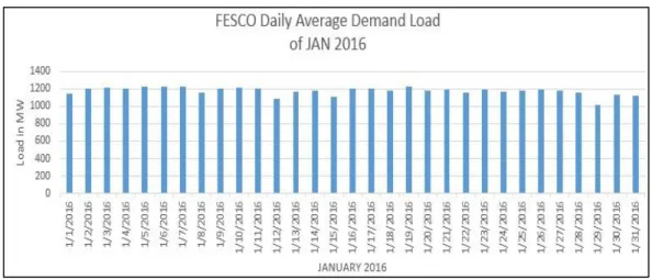
Figure 2.2: FESCO daily average demand load of January 2016 [2]

Source: H.S Hippert, C. E. Pedreira and R. C. Souza, 2005 [2].

Figure 2-2 shows a significant difference in a daily average demand load of FESCO for the month of January 2016. Since in Faisalabad city Friday is considered as a holiday by the majority of textiles, industries, and markets. A major difference can be seen in demand load for 1/1/2016, 1/8/2016 and vice versa because of Fridays. Table 2-1 represents the average demand load of FESCO for different days of the week in the year 2016.

(21)

7

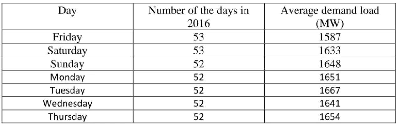
Table 2.1: FESCO Average demand load for each day in 2016

Day Number of the days in

2016

Average demand load (MW) Friday 53 1587 Saturday 53 1633 Sunday 52 1648 Monday 52 1651 Tuesday 52 1667 Wednesday 52 1641 Thursday 52 1654

Source: H.S Hippert, C. E. Pedreira and R. C. Souza, 2005 [2].

2.2.2 Weather Factor

Weather factor has a significant effect on the short-term electric load forecasting of a power system. And according to electric load prediction survey [3] published, air temperature is the most important factor considered for short-term load forecasting model. Weather-sensitive loads, such as heating, ventilating, and air-conditioning (HVAC) equipment, strongly affects the power systems as these electrical loads tend to be the larger loads on the system. Switching on and off HVAC apparatus can produce electrical load profiles that appear to have random power swings. In figure 2-2 the electric load peak occurs at 2596MW in the last week of June when the average air temperature is close to its maximum. And also, the bottom average demand load occurs at 960MW during the second week of December when the average air temperature is close to its minimum.

Table 2-2. Shows the average demand load and air temperature of the last week of June 2016 and Table 2-3. Shows the average demand load and air temperature of the second week of December 2016.

(22)

8

Table 2.2: FESCO demand load of summer week in 2016 [3].

Date Average demand load (MW)

Average air temperature (°C)

6/24/2016 2332 39 6/25/2016 2466 42 6/26/2016 2366 38 6/27/2016 2224 38 6/28/2016 2118 35 6/29/2016 2501 38 6/30/2016 2596 39

Source: Eugene A. Feinberg and Dora Genethliou, 2006 [3].

Table 2.3: FESCO demand load of winter week in 2016 [3].

Source: Eugene A. Feinberg and Dora Genethliou, 2006 [3].

2.2.3 Random Factor

Random factors that affects the electrical load profile contains all the random interferences in the load pattern that cannot be expressed by weather and time factor. The random factor can consist of significant loads which occur randomly having no operating schedule which makes prediction difficult. Random factor includes planned or unplanned electric load shedding, festival or event, etc.

Date Average demand load (MW) Average air temperature (°C)

12/8/2016 1174 20 12/9/2016 1044 18 12/10/2016 1110 21 12/11/2016 1030 20 12/12/2016 960 20 12/13/2016 1073 21 12/14/2016 1170 21

(23)

9

2.3 LOAD FORECAST METHODS

Since load forecasts can be divided into four types which are discussed in section 2.1 having different time spans, therefore this means that for each of the type, there will be the most appropriate methods to operate the forecast models. For MTLF and LTLF, the so-called end-use and econometric approach are broadly end-used. For VSTLF and STLF several methods are used and most of these methods are discussed in this research.

2.3.1 Multiple Linear Regression (MLR)

Multiple linear regression utilizes two or more explanatory variables and a response variable by fitting a linear equation to the observed data and seeks to represent the linear relationship between them. This method uses explanatory weather and non-weather variables to predict the electrical load at a specified time t. These variables tend to have a great impact on electrical load and are selected by correlation analysis with the load [7]. Regression coefficients are calculated by using least square estimation techniques. And these coefficients are multiplied by the variables [8]. Every value of the dependent variable y is associated with a value of the independent variable x.

The MLR electrical load model has the following form:

y(𝑡) = 𝑎0 +a1(𝑡) + . . . + 𝑎𝑛𝑥𝑛(𝑡) + 𝑎(𝑡) (2-1)

where,

y(𝑡) = electrical load

𝑥1(𝑡) … 𝑥𝑛(𝑡) = explanatory variables correlated with 𝑦(𝑡)

a(𝑡) = a random variable with zero mean and constant variance. 𝑎0, 𝑎1,.…, 𝑎𝑛 = regression coefficients.

2.3.2 Time Series

Time series can be defined as a sequential set of data measured over time, such as the hourly, daily or weekly peak load. It uses historical load data to predict the future load [9]. The electric load y(t) is modeled as the output of a linear filter with a random series input a(t) also

(24)

10

called white noise. This random input has a zero mean with fixed unknown variance σa2 (t).

Different models of STLF can be classified depending on the characteristic of the linear filter [10].

Figure 2.3: Load time series modeling [10].

White Noise

a(t)

Source: T.G. Manohar and V.C. Veera Reddy, 2008 [10].

The Autoregressive (AR) model defines the forecasted electric load y(t), in terms of the previous load values and a random noise signal a(t) [11].

y(𝑡) = 𝜙1𝑦 (𝑡 − 1) + 𝜙2𝑦 (𝑡 − 2) + . . . + 𝜙𝑝𝑦 (𝑡 − 𝑝) + a(𝑡) (2-2)

The Moving-Average (MA) model defines the forecasted electric load y(t), in terms of the current and previous values of series of random noise signals. This noise series is constructed from the forecast errors or residuals when load observations become available [11].

y(𝑡) = a(𝑡) − 𝛩1𝑎 (𝑡 − 1) − 𝛩2𝑎 (𝑡 − 2) − . . . − 𝛩𝑞1𝑎 (𝑡 − 𝑞) (2-3)

The Autoregressive Moving-Average (ARMA) model defines the forecasted electric load y(t), with the combination of AR and MA model.

y(𝑡) = 𝜙1𝑦 (𝑡 − 1) + 𝜙2𝑦 (𝑡 − 2) + . . . + 𝜙𝑝𝑦 (𝑡 − 𝑝) + (𝑡) − 𝛩1𝑎 (𝑡 − 1) − 2𝑎 (𝑡 − 2) –

………𝛩𝑞1𝑎 (𝑡 − 𝑞) (2-4)

Linear Filter

(25)

11

The AR, MA and ARMA processes are also called stationary process. If the process is non-stationary, a transformation is required which is achieved by differences in ARMA model. The transformed model is called Autoregressive Integrated Moving Average (ARIMA) model.

The Transfer Function (TF) model uses AR, MA, ARMA or ARIMA model to represent white noise and load data with one or more variables such as air temperature, wind speed, humidity, etc. which tends to have a strong effect on electric load profile [11]. Using a TF these other variables can be modeled as shown below in Figure 2-4.

Figure 2.4: Transfer function (TF) model [11].

Source: Z. H. Ashour, M. A. Abu El-Maged and M. A. El-Fattah Farahat, 1991[11].

2.3.3 Expert System

An expert system is a computer-based program comprising a large historical database and a set of rules which are used to search the historical database for the best solution to a particular problem. Expert systems are an emerging technology with many fields such as STLF [11]. The expert systems are followed by IF-THEN rules and mathematical expressions which are used to make forecasts. Some rules have to be updated continually while others do not change over time [12]. Input x(t) White Noise a(t) Transfer Function Model Noise Model + n(t) y(t)

(26)

12

2.3.4 Similar-day Approach

The similar-day approach is widely used for STLF. This approach investigates historical database for same characteristics to the forecasted day. Same characteristics include dates, weather, the day of the week, etc. A load of same day matching the characteristics is considered as a forecast. Though many days can match the characteristics, various techniques have been developed and used to reduce the error and improve the efficiency of forecast [13].

2.3.5 Neural Networks

Neural Networks (NN) or Artificial Neural Network (ANN) method has been widely studied and used for load forecasting since 1990 [14]. Neural networks are essentially non-linear circuits that have the demonstrated capability to do non-linear curve fitting. A neural network is a machine that is designed to model the way in which the human brain performs a particular task. The brain is a highly complex, nonlinear and parallel information processing system. As there are billions of neurons in the human brain, ANN basic processing components are the neurons. These neurons are programmed to act similarly to the neurons in the brain by receiving an input, performing a particular task based on the input and produce an output. Chapter 3 discusses the Neural Networks in detail.

2.4 TYPES OF NEURAL NETWORKS

There are several types of Neural Networks each based on different architecture. Neural Networks can be further classified in to 4 general categories being preferred and used in machine learning. Given below are the types of Neural Networks:

2.4.1 Feed Forward Neural Network

Though it can be understandable by the term feed forward which means that the direction or information given flows in a forward one direction. This approach became practical in 1950’s [15]. In FF network, all the nodes are fully connected and the data flows from input layer to output layer without any back loops. Given below is the figure of FF network with one hidden layer.

(27)

13

Figure 2.5: Feed forward neural network [15]

Output Layer

Input Layer Hidden Layer

Source: Chen H, Canizares C.A and Singh A, (2001).

The hidden layers can be varied according to the requirements. In this research, a MLP method is used for STLF which is briefly discussed in chapter 3. The function of these three input, hidden and output layers are also briefly discussed.

2.4.2 Recursive Neural Network (RNN)

Recursive Neural Networks (RNN) are non-linear adaptive models having the ability of learning deep structured information. They were introduced in late 90’s [17]. These computational models are suited for both regression and classification problems being capable of carrying non-supervised and supervised training tasks. The most popular algorithm used to train the RNN is the back-propagation method. Back-propagation method is also briefly discussed in the next chapter.

(28)

14

Figure 2.6: Simple recursive neural network architecture [17]

S

WScore P1,2

W

C1 C2

Source: Frasconi P, Gori M and Sperduti A, 1997 [17]

The network is made by applying the same set of weights recursively over a structure to make a structured forecast over variable-size input structures by traversing the provided structure in topological order. Recursive Neural Networks are very powerful in learning hierarchical, tree-shape structures. These models have not been broadly accepted, due to their inherent complexity. And also due to the fact of computationally expensive training phase. RNN has been found not to the best appropriate for structured processing due to the convergence problem [18]. In figure 2-6, if C1 and C2 are n-dimensional vector representing nodes, their

parent p will also be an n-dimensional vector, calculated as:

P1, 2 = tanh (W[c1;c2])

(2-5)

(29)

15

2.4.3 Convolutional Neural Network (CNN)

Convolutional Neural Network consists of one or more than one convolutional layers partially or fully connected and utilizes a variation of Multilayer Perceptron (MLP) which are discussed in the next chapter.

Figure 2.7: Typical convolution neural network architecture [19]

Source: Y. Bengio, R. Ducharme and P. Vincent, 2003 [19]

As it can be viewed from Figure 2-7 given above, CNN uses several convolution layers for carrying out the output. In these layers convolution operation is applied passing the results to the next layers. This method allow the network to be deeper with much fewer parameters. CNN shows tremendous results in image and speech applications [19].

2.4.4 Recurrent Neural Network

Recurrent Neural Networks are unlike a FF neural network, is an alternate of RNNs in which the connection between neurons makes a directed cycle. The first network of this type was called Jordan Network, when each of the hidden cell recieved its output with fixed delay. In this network, the output depends not only on the present inputs but also on the previous step’s neuron state [20].

(30)

16

Figure 2.8: Recurrent neural network architecture [20]

Input Layer Hidden Layers Output Layer

Source: Mesnil G, He X, Deng L and Bengio Y, (2013) [20]

Figure 2-8, represents the architecture of recurrent neural network. The memory lets the users to solve non linear problems like speech recognition and connected handwriting and text classifications. The most common examples of recurrent neural network are texts , a word can be analysed only in context of previous words or sentences.

(31)

17

3. SHORT-TERM LOAD FORECAST USING ANN

ANNs have received an extensive share of the research attention in STLF since the late 1980’s. Artificial Neural Networks are mathematical tools or computer-based programs that mimic the way human brain processes information [14]. The basic processing element in neural networks is neurons. In ANNs a group of artificial neurons is interconnected and processes information using a connectionist approach to computation. The neuron is shown mathematically in Figure 3-1.

Figure 3.1: An artificial neuron model [14]

Source: Resource: Chen H, Canizares C.A and Singh A, (2001) [14]

As shown in above Figure 3-1, a neuron model consists of a combination of inputs represented by Xi each having unique weights Wi which are associated with those inputs.

Additionally, there is another constant input 1 having its unique weight b also called the bias. The main function of bias is to provide every input node Xi with a trainable constant value.

The output (y) of a neuron is computed as:

y= f (X1W1+X2W2+XmWm+b) (3-1)

The linear combination of all these inputs (XiWi+b) is given as an input to a function. This

function is called the activation function as shown in Figure 3-1 above. The activation function is a non-linear function. The reason behind this is that the training of ANN requires

(32)

18

the activation function to be differentiable and not decreasing [15]. It is important because of the fact, that most real-world data is nonlinear and we want neurons to learn these nonlinearities. There are several activation functions. Every activation function takes the single input and performs certain fixed mathematical operations [15]. Some of the activation functions are given below:

i. Sigmoid Function: This activation function receives the input and distributes it to range between 0 and 1. The mathematical expression of the sigmoid function is given below:

σ(x)=_1+𝑒1_−𝑥 (3-2)

ii. tanh Function: This activation function takes a real-valued input and divides it to the range [-1, 1]. The mathematical expression of this function is given below:

tanh(x)=2σ(2x)–1 (3-3)

iii. ReLU Function: ReLU stands for Rectified Linear Unit. This type of activation function receives a real-valued input and thresholds it at zero (replaces negative values with zero)

f(x)=max(0,x) (3-4)

(33)

19

Figure 3.2: Different activation functions [15]

Source: H.S. Hippert, C.E. Perdreiraand R.C. Souza, 2001 [15]

The architecture of an ANN tells that how its several neurons are placed in relation to each other. These arrangements are structured essentially by directing the synaptic connections of the neurons. In general, the architecture of ANN can be divided into three parts, named layers, which are given below:

i. Input Layer: The process of the input layer is to receive the data or information provided and pass it to next layer which is called hidden layer. The data is normalized to limit values produced by the activation functions.

ii. Hidden Layer: The data or information received in the input layer is passed to the hidden layer. Hidden layer has no direct access to outside world. The process of hidden layer is to extract patterns associated with the task or system being analyzed. Most of the internal processing from a network is performed in hidden layers. A feedforward network will only have a single input layer and a single output layer, it can have zero or multiple Hidden Layers.

iii. Output Layer: The data or information passed from the hidden layer is finally processed in the output layer. This layer is responsible for computations and presenting an output to a network created.

(34)

20

The main architecture of ANN can be divided into single-layer feedforward, multilayer feedforward, recurrent and mesh networks [16]. In a feedforward network, data or information provided travels in only one direction. This research uses a multilayer feedforward network which is discussed in next section.

3.1 MULTILAYER PERCEPTRON

Multilayer Perceptron or Multi-layer feedforward neural network has an input layer, one or more hidden layers, and an output layer. While, when one hidden layer is enough to learn the linearity, multilayer perceptron is used to also learn the non-linearity in the given data or information [15]. Figure 3-3 given below shows the feed-forward network with multiple inputs.

Figure 3.3: Multi-layer feedforward network [15]

(35)

21

X1, X2,..., Xn is the data or information given to the input layer of the network. The network

has multiple hidden layers with n neurons. Finally, one output neural layer composed of m neurons representing the respective output values of the problem being analyzed.

3.2 NETWORK TRAINING

Artificial Neural Networks are produced by using some training algorithms. There are generally three classes for training ANNs:

1. Supervised Learning

In supervised learning, each training sample comprises of input data and their corresponding outputs. Supervised learning is further grouped into regression and classification problems. The training algorithms use mathematical operations to learn the relation between input and output. Backpropagation (BP) algorithm is mostly used for training ANNs under supervised class which is discussed later in this chapter [16].

2. Unsupervised Learning

In unsupervised learning, there is only an input data x and no corresponding output data. According to the inputs provided to the network, the weights are changed. ANN treats the set of data or information provided as a random variable. The network then provides a solution using those random variables [21]. Unsupervised learning technique is further grouped into clustering and association problems.

3. Semi-Supervised Learning

In semi-supervised learning, there is an input data x and only some of the output data is labeled y. A combination of supervised and unsupervised techniques can be used in semi-supervised learning.

(36)

22

3.3

BACKPROPOGATION ALGORITHM

Backpropagation (BP) algorithm is mostly used for training ANNs under supervised class [16]. ANNs consists of nodes in different layers, which includes input, hidden and output layers. As shown in Figure 3-1 and Figure 3-3, nodes of different adjacent layers have “weights” associated with them. For assigning correct weights training is required. And since ANNs can have multiple hidden layers, assigning correct weights to multiple hidden layers can be a complex task. This task is achieved by using Backpropagation (BP) algorithm. BP algorithm is based on Widrow-Hoff delta learning rule. In this method, initially, all weights and bias for different hidden layers are randomly assigned. The data or information is provided to the network, the ANN is activated and an output is noted down. This output is then compared with the target output and an error is generated. The generated error is then propagated back to hidden layers and weights are adjusted accordingly. The process keeps on repeating until the minimum error is achieved. The training process flowchart using backpropagation algorithm is shown in Figure 3-4.

(37)

23

Figure 3.4: Backpropagation training flowchart [16]

Source: M. Ramezani, H. Falaghi, and M. Haghifam, 2005 [16]

The backpropagation training process is described in ten steps given below [16]: i. Network weights are initialized.

ii. Add the weighted input and apply activation function to calculate the output of the hidden layer.

hj = f [Ʃi XiWij] (3-5)

where,

hj is the output of hidden neuron j for i inputs

xi is the input data of input neuron i

Wij are the synaptic weights between input neuron i and hidden neuron j

(38)

24

iii. Add the weighted output of hidden layer and apply activation function to calculate the output of the output layer.

Ok = f [ Ʃj hj Wjk ] (3-6)

where,

Ok is the output of output neuron k

Wjk is the synaptic weight between hidden neuron j and output neuron k

iv. Calculate back propagation error.

𝛿k= (tk - Ok ) f’ ( Ok ) (3-7)

where,

f’ is the derivative of the activation function tk is the target of output neuron k

v. Compute the weight correction term

∆Wjk (n) = ƞ𝛿khj + ɑ∆Wjk (n-1) (3-8)

where,

ƞ is the training ratio ɑ is the moment coefficient

vi. Add the delta input for each hidden neuron and generate an error 𝛿j = Ʃk 𝛿k Wjk f’ ( Ʃi Xi Wij ) (3-9)

vii. Compute weight correction term

∆Wij (n) = ƞ𝛿jXi + ɑ∆Wij(n-1) (3-10)

viii. Update the weights

Wjk (n+1) = Wjk (n) + ∆Wjk (n) (3-11)

Wij (n+1) = Wij (n) +∆Wij (n) (3-12)

ix. Repeat step (ii) for the following number of errors:

MSE= _2𝑝1

[

ƩpƩk (dpk - Opk)2] (3-13)

where,

p is the patterns in the training set and MSE is the mean square error x. Training is ended.

(39)

25

Even though the backpropagation method is very efficient for training MLP or feedforward neural networks, but the training process takes a lot of time due to the nature of gradient descent [22]. There are many methods produced to refine the backpropagation algorithm, and one of them is the Levenberg-Marquardt (LM) algorithm. Levenberg Marquardt combines the speed of Gauss-Newton’s method and the stability of error backpropagation algorithm during training steps. This research uses Levenberg-Marquardt algorithm for training and creating an ANN.

To reduce the overtraining and hence preventing the overfitting factor cross-validation process is adopted. Cross-validation process divides the training data set into a test set and validation set. Data or information set provided to ANN is trained using the test set and tested after every few iterations using the validation set. When the validation set performance starts to decrease training is completed [15].

An ANN for load forecasting can be trained on a training set of data that consists of time-lagged load data and other non-load parameters such as weather data, time of day, the day of the week, month, and actual load data [3] [24]. In this research, the time-lagged data of average demand load and the average air temperature was created as shown Table 3-1. The important data was selected through two different methods discussed in the next section of this chapter. In Table 3-1, Avg Load in MW represents the target data and the Avg Temp to Prev2 Temp in °C represents the input time-lagged data.

(40)

26

Table 3.1: Time-lagged load and air temperature data [1]

Date Avg. Load (MW) Avg. Temp (°C) Prev1 Load (MW) Prev2 Load (MW) Prev3 Load (MW) Prev4 Load (MW) Prev5 Load (MW) Prev1 Temp (°C) Prev2 Temp (°C) 1.06.2016 1227 18 42374 42373 1214 1200 1146 22 19 1.07.2016 1229 20 42375 42374 1208 1214 1200 18 22 1.08.2016 1159 20 42376 42375 1221 1208 1214 20 18 1.09.2016 1200 22 42377 42376 1227 1221 1208 20 20 1.10.2016 1216 22 42378 42377 1229 1227 1221 22 20 1.11.2016 1205 18 42379 42378 1159 1229 1227 22 22 1.12.2016 1086 15 42380 42379 1199 1159 1229 18 22 1/13/2016 1170 18 42381 42380 1216 1199 1159 15 18 1/14/2016 1176 18 42382 42381 1205 1216 1199 18 15 1/15/2016 1105 18 42383 42382 1085 1205 1216 18 18

Source: Y. Al-Rashid and L.D. Paarmann, 1996 [1].

The predictor variables are the time-lagged load and weather data which is the average air temperature, given as an input of ANN. Forecast error is calculated by comparing the forecasted load generated by ANN with the actual load. Forecast error is often presented in terms of the Root Mean Square Error (RMSE) with units of kW [2] [15] as shown in (3-14), but more commonly in terms of the Mean Absolute Percent Error (MAPE) with units of percent [2] [15] [24] as shown in (3-15) RMSE = √_𝑁1 𝑥 ∑𝑁_𝑡=1(𝑦_𝑡− ӯ_𝑡)² (3-14) MAPE = _𝑁1 𝑥 ∑ ( |𝑦𝑡−ӯ𝑡| 𝑦𝑡 𝑥 100) 𝑁 𝑡=1 (3-15) in which,

(41)

27 𝑁 is the number of samples,

𝑦𝑡 = target load at time 𝑡

ӯt = forecasted load at time t

An ANN created with particular input load and weather data will be system dependent. The network created with one system, will more likely not give satisfactory results on another system due to different properties. However, the same ANN architecture may be reused on the new system, but retraining will be required [15].

3.4 DATA-PREPROCESSING

All ANNs have random mapping capacities theoretically, but before the training process, it is appropriate to normalize the data for certain scaling differences between the variables [25]. Since there are many highly correlated variables but many of them do not provide a relevant information extracted from the data. These uncorrelated variables decrease the learning performance of the neural network. To overcome these uncorrelated variables several methods have been used so far. Neural network training can be made more efficient if certain preprocessing steps are performed on the network inputs and targets [22].

Since providing an appropriate set of inputs will reduce the overfitting factor and increase the efficiency of ANN. And to achieve this two methods Correlation and Relief was used in this research.

3.4.1 Correlation Analysis

Correlation is a statistical tool that is used to determine the relationship between two variables. The statistic is called a correlation coefficient [26]. A correlation coefficient describes the direction (positive or negative) and degree (strength) of the relationship between two variables. A correlation coefficient can vary from -1.00 to +1.00. Correlation

(42)

28

coefficient closer to 0 represents less relationship. The correlation coefficient is achieved by calculating the covariance between input variable x and target variable y and standard deviation of each variable. Equation (3-16) shows how to calculate the correlation between two variables x and y

r(x,y) =

𝐶𝑂𝑉(𝑥,𝑦)

SxSy (3-15)

r(x,y) represents the correlation of the variables x and y, whereas COV(x,y) is the covariance of

the variables x and y. Sx and Sy are the standard deviations of random variables x and y

respectively.

Figure 3-5 shown represents the one-year correlation between FESCO electric demand load and average air temperature.

Figure 3.5: One-year correlation between electric demand load and average air temperature [10]

Source: Z. H. Ashour, M. A. Abu El-Maged and M. A. El-Fattah Farahat, 1991 [10]

0 500 1000 1500 2000 2500 3000 0 5 10 15 20 25 30 35 40 45 50 LO AD IN M W

Average Air Temperature in °C

(43)

29

3.4.2 Relief Method

Relief algorithm is considered among the most successful one for the selection of features due to its simplicity and effectiveness. The basic function of Relief algorithm is to iteratively estimate feature weights according to their ability to distinguish instances located near each other [27]. For distinctive instances, the algorithm iteratively selects a random instance and after that searches for its two nearest neighbors - the nearest hit (NH) from the same class and the nearest miss (NM) from the different class. The difference between the current instance and its NH and NM along the corresponding attribute axis will result in the estimation of weight for each feature. Relief algorithms perform better than other filter methods because of the feedback performance of a nonlinear classifier when searching for important attributes [28]. Relief method is used for classification problem, whereas the ReliefF is the upgraded Relief used for the regression problems since the target values are continuous variables in regression tasks [27].

The pseudo code for the Relief algorithm is given below:

1: set W[A] = 0; set all feature Weights(W[A]) to zero 2: for i := 1 to m do

3: select an instance Ri randomly

4: find nearest hit NH and nearest miss NM; (instances) 5: for A := 1 to a do

6: W[A] := W[A] - diff(Ri[A],NH[A]) + diff(Ri[A],NM[A]);

7: end for 8: end for

a is the number of attribute(features) n is the total number of instances

m is the random training instance selected from n

ReliefF method is used in the research for the selection of important features on regression problems. There are two major drawbacks to Relief method that they are computationally expensive and they may fail to remove the unimportant variables, which results in poor forecast while used as an input [28].

(44)

30

In this research both of the methods, Correlation analysis and Relief method are used to extract an important set of useful data in forecasting day-ahead demand load. And this task is achieved by a commercial machine learning software named “WEKA”. In WEKA, all the data is imported first by means of file conversion. And after that by choosing both methods individually, results are driven rankly. Chapter 4 shows the results for both methods and as well as the results of day-ahead load forecast for FESCO.

(45)

31

4. RESULTS AND DISCUSSIONS

This chapter presents the scatter plots created to visualize the relationship and drift between electric load and the predictor inputs. This chapter also shows the results of the time-lagged load and historical air temperature data used to extract important attributes set by means of two methods, Correlation analysis and Relief method. The best attributes set is later used to forecast day-ahead load using ANN. The results of day-ahead load forecast are also shown in this chapter. And at the end discussions are made using the achieved results.

4.1 SELECTION OF INPUT VARIABLES

In order to achieve an adequate fit for the network, the dataset is first refined using two different techniques Correlation and Relief method. And this task was achieved with the aid of Commercial Software “WEKA”. The results are given below for both methods:

4.1.1 Relief Method

The created time-lagged load data comprising a load of previous five days along with their averages and derivative differences, same with the historical weather data, all were given as an input test set to WEKA®. The target dataset y was selected. And by using different values of nearest neighbors k, results are displayed by means of the Ranker method. Ranker method is only capable of producing a ranked list of attributes for attribute evaluators. Given below are the results of attribute evaluator using Relief Method for different values of nearest neighbors k.

(46)

32

Table 4.1: Top-ranked variables by ReliefF attribute evaluator k=10 [27]

VARIABLES RANK

Prev1 Load 0.036469

1st Dev Load Prev1 0.035651 Avg Prev 1-2 Load 0.025734 1st Dev Load Prev2 0.021467 1st Dev Load Prev3 0.021379

Prev2 Load 0.021000

Prev5 Load 0.020613

Avg Prev 1-3 Load 0.020574 Precipitation in mm 0.018991 Avg Prev 1-5 Load 0.018762

Source: Kira K and Rendell L, 1992 [27]

VARIABLES RANK

Prev1 Load 0.039570

1st Dev Load Prev1 0.034740 Avg Prev 1-2 Load 0.029290 Avg Prev 1-3 Load 0.023900

Prev2 Load 0.022930

Prev5 Load 0.022020

Avg Prev 1-5 Load 0.021670 Avg Prev 1-4 Load 0.021440 1st Dev Load Prev2 0.020970 1st Dev Load Prev3 0.020680 Source: Kira K and Rendell L, 1992 [27]

(47)

33

Table 4.3: Top-ranked variables by ReliefF

attribute evaluator k=30 [27]

VARIABLES RANK

Prev1 Load 0.042096

1st Dev Load Prev1 0.034114

Avg Prev 1-2 Load 0.031304

Prev2 Load 0.024452

Prev5 Load 0.022440

VARIABLES RANK

Prev1 Load 0.043610

Prev2 Load 0.025349

Prev5 Load 0.023014

Prev3 Load 0.020718

(48)

34

As shown from Table 4-1 to Table 4-4, depending on the nearest neighbors k different variables are displayed rankly showing a connection with output variable y.

For each value of k (10, 20, 30, 40, 50), test sets were made from the results shown in Table 4-1 to Table 4-4. In the beginning, total 5 test sets were selected comprising 10 to 14 variables respectively and were utilized as an input to ANN. Matlab® aided the work with ANNs. The hidden layers were varied from 15 to 25 in order to minimize the training error. Later in this chapter, selection of hidden layers are also discussed. The network was trained using LM algorithm. The results of attributes set depending on the nearest neighbor k are shown in the Table 4-5 given below:

Table 4.5: MAPE for different variables set for different values of k [27]

nearest neighbors (k) MAPE % 10 Variables MAPE % 11 Variables MAPE% 12 Variables MAPE % 13 Variables MAPE % 14 Variables k=10 3.999 3.96 3.88 4.2541 3.471 k=20 4.1712 3.91 3.88 3.7456 3.7289 k=30 4.2657 4.15 3.76 3.2056 3.871 k=40 4.3225 3.98 4.22 3.7581 3.7439 k=50 4.2038 4.17 4.2 3.9686 3.662

From Table 4-1, it can be seen that the minimum MAPE is achieved for the nearest neighbors k=30. The minimum MAPE is 3.2% for a 13 variable test set. This information was recorded and the test set was saved for the later operations.

(49)

35

4.1.2 Correlation Analysis

Pearson correlation coefficient was used to calculate the magnitude of the linear correlation between electric demand load and weather data, electric demand load and time-lagged load and weather data. This method was also performed with the aid of commercial software “WEKA”. Results of this method are shown below in Table 4-6:

Table 4.6: Correlation analysis between electric load and time -lagged load and weather data [26]

VARIABLES RANK

Prev1 Load 0.96720

Prev2 Load 0.93618

Prev3 Load 0.91368

Prev4 Load 0.89580

Prev5 Load 0.88734

Avg Temp 0.87117

Source: H. Almuallim and T. G. Dietterich, 1992 [26]

As shown in Table 4-5, the load of the previous day is highly correlated with the target load y. The value for previous day load is 0.9672. And this correlation tends to decrease as the time span increases. The average air temperature is also highly correlated with the value of 0.87117 as shown in Figure above.

Utilizing the results achieved with correlation analysis shown in Figure 4-5, 12 test sets were created comprising 3 to 14 variables respectively. Each test set was given as an input to ANN.

(50)

36

These samples were further divided into training, validation and testing set. The number of samples were 547 which were further divided 80% for training and 20% for testing. After training the network, results were gathered in terms of MAPE% shown in Table 4-7 below.

Table 4.7: MAPE for different input variables test sets

Number of Variables (n) n=3 n=4 n=5 n=6 n=7 n=8 n=9 n=10 n=11 n=12 n=13 n=14 MAPE (%) 6.03 6.81 5.93 6.36 6.33 6.45 6.28 5.19 5.78 5.06 5.38 5.35

Source: H.S Hippert, C. E. Pedreira and R. C. Souza, 2005 [2]

In Table 4-7, less data was given as an input to ANN as compared to the data provided to ANN, the results are shown in Table 4-8.

In table 4-8, the training set contains 383 samples, while validation and testing both sets contain 82 samples. The hidden layers were varied from 15 to 25 in order to acquire better results by reducing the MSE.

After training the network results were gathered in terms of MAPE shown in Table 4-6 below. The minimum MAPE 3.07% was achieved for the test set with 12 variables.

Table 4.8: MAPE for different input variables sets

Number of Variables (n) n=3 n=4 n=5 n=6 n=7 n=8 n=9 n=10 n=11 n=12 n=13 n=14 MAPE (%) 4.45 4.33 4.36 4.17 4.22 4.21 4.35 3.86 3.63 3.07 3.38 3.44

(51)

37

Even though the Relief method is considered among the best methods [28] for providing an attribute set highly related to the target set. But for our custom (FESCO) data, Correlation method provides the best of all with a MAPE of 3.07%, which comes in the acceptable range as discussed in Section 2.2 [1].

4.2 PREDICTOR SCATTER PLOTS

Scatter plots helps in visualizing and understanding a linear relationship between target variable y and input variables x. Given below are the scatter plots for the electric demand load and time-lagged load and weather data.

Figure 4.1: Scatter plot between electric load and previous 4 days load [10]

(52)

38

From Figure 4-1, it can be seen that the previous day load is highly correlated with the electric load. While on the other hand, this correlation tends to decrease with the increase in the time span. Previous 4th Day Load shows a less relationship than the previous day load.

Figure 4.2: Scatter plots between electric load and previous 4 days average air temperature [10]

(53)

39

From Figure 4-2, the relationship between electric load and previous 4 days can be seen. The previous day daily average air temperature is more correlated than the previous 4th-day air temperature.

Figure 4-3 and Figure 4-4 show the scatter plots between electric load and each month of the year and electric load and each day of the week.

Figure 4.3: Electric load and month of year scatter plot

0 500 1000 1500 2000 2500 3000 0 2 4 6 8 10 12 14 LOAD in M W Month of Year

(54)

40

Figure 4.4: Electric load and day of week scatter plot [10]

From Figure 4-3, it can be that maximum demand load occurs in the mid of the year. While on the other hand, electric load demand for the month of December is minimum. Figure 4-4, shows that the peak demand load occurred for the 6th day of the week which is Thursday. As mentioned earlier in chapter 2, Friday is considered as a holiday for FESCO.

4.3 SHORT-TERM LOAD FORECAST RESULTS AND DISCUSSIONS

The results gathered by the Correlation analysis were further used to create an ANN comprising 547 samples. The results are shown in Table 4-2. Using this information, first of all, the test set comprising 547 samples representing all days were divided into each day of the week.

Each ANN representing each day of week contains 78 samples which were further divided into 70 percent for the training set, 15 percent for validation set and 15 percent for testing set. Figure 4-6, shows MATLAB® Neural Network tool plot. The input of Neural Network

0 500 1000 1500 2000 2500 3000 0 1 2 3 4 5 6 7 8 Lo ad in MW Day of Week

(55)

41

contains 12 inputs, hidden layers were fixed to 18 and 1 output layer representing day-ahead load forecast for each individual day.

Each training cycle is called an Epoch. In general, the error reduces after more training epochs but might increase on the validation set. By default, the training stops after six consecutive increases in a validation error. The training of Neural Network stops if the number of an epoch is completed or the performance on the validation set reaches its minimum.

Figure 4.5: MATLAB® neural network tool plot [22]

(56)

42

Figure 4.6: MATLAB® training state plot [22]

Source: Demith H and Beale M, (1998) [22]

Figure 4-6, given above represents three different graphs. The top graph shows the drift in gradient values for each number of the epoch. After 6 epochs the graph for gradient values decreases gradually. The middle plot shows the learning rate (mu) for each epoch number. The graph decreases gradually until 5 number of epochs and becomes constant after that. The last plot shows the plot of validation checks against each number of the epoch. A sudden change in gradient plot is observed at validation plot.

(57)

43

Figure 4.7: MATLAB® regression plot [22]

Source: Demith H and Beale M, (1998) [22]

Figure 4.7 shows the regression plot of Thursday data for day-ahead load forecast. The regression plot contains a plot of training, validation, and testing states. A solid line represents the best fit between output and target data. The dotted line represents the targets which are results-output. Each circle represents data. R values tell the relationship between output and the target value. If R is close to 1, it reveals the perfect linear relationship between outputs and targets. From the regression plot R=1 for training, R=0.99 for validation, R=0.99 for testing and R=0.99 for all. The R-value almost 1 for all sets represents satisfactory results for forecasting.

The data samples were further divided into training, validation and testing set. The number of samples were 78 which were further divided 80 percent for training and 20 percent for testing. After training the network, results were gathered in terms of MAPE% shown in Table 4-9 below.