REPUBLIC OF TURKEY
YILDIZ TECHNICAL UNIVERSITY
GRADUATE SCHOOL OF NATURAL AND APPLIED SCIENCES
DÜZLEMSEL HOMOTETİK HAREKETLER ALTINDAT.C.
YILDIZ TEKNİK ÜNİVERSİTESİ
FEN BİLİMLERİ ENSTİTÜSÜ
ROBUST CLASSIFICATION BASED ON SPARSITY
ELENA BATTINI SÖNMEZ
DANIŞMANNURTEN BAYRAK
THESIS FOR THE DEGREE OF DOCTOR OF PHILOSOPHY
COMPUTER ENGINEERING DEPARTMENT
YÜKSEK LİSANS TEZİ
ELEKTRONİK VE HABERLEŞME MÜHENDİSLİĞİ ANABİLİM DALI
HABERLEŞME PROGRAMI
ADVISOR
ASSISTANT PROF. DR. SONGÜL ALBAYRAK
İSTANBUL, 2011DANIŞMAN
DOÇ. DR. SALİM YÜCE
ISTANBUL, 2011
REPUBLIC OF TURKEY
YILDIZ TECHNICAL UNIVERSITY
GRADUATE SCHOOL OF NATURAL AND APPLIED SCIENCES
ROBUST CLASSIFICATION BASED ON SPARSITY
Presented by Elena BATTINI SÖNMEZ on 22.12.2011 and accepted by the following committee on behalf of the Computer Engineering Department, Yıldız Technical University, in partial satisfaction of the requirements for the DEGREE of DOCTOR of
PHILOSOPHY. Thesis’s Advisor
Assist. Prof. Dr. Songül Albayrak Yıldız Technical University
Jury's Members
Assist. Prof. Dr. Songül Albayrak
Yıldız Technical University _______________________
Prof. Dr. Bülent SANKUR
Boğaziçi University _______________________
Prof. Dr. Hasan Dağ
Kadır Has University _______________________
Prof. Dr. A. Çoşkun Sönmez
Yıldız Technical University _______________________
Assist. Prof. Dr. Güneş Karabulut Kurt
ACKNOWLEDGEMENTS
This thesis is the result of several years of work, impossible to accomplish without the help of many people. I take this opportunity to thank all of them.
I thank very much my advisor, Assist. Prof. Songül Albayrak, for being always present at my side, and giving me precious advice as well as the moral to overcome difficulties. It would have been very difficult to complete this research without her encouragement. I thank very much Prof. Bülent Sankur for the big effort in teaching and directing me in this research. I am very grateful for the enormous amount of time spent with me discussing different problems ranging from theoretical issues down to technical details. My special thanks to my family, who kept the joy in my life.
Finally, I would like to thank the family of my husband, for the never ending help, all my friends for being always nearby me, and all of my colleagues at Istanbul Bilgi University for their patient understating of my overwhelming schedule.
August, 2011
v
CONTENTS
Page
LIST OF SYMBOLS vii
LIST OF ABBREVIATIONS viii
LIST OF FIGURES x
LIST OF TABLES xii
ABSTRACT xiii
ÖZET xiv
CHAPTER 1 INTRODUCTION
1.1 Literature Review 1
1.2 Aims of the Thesis 5
1.3 Hypothesis 6
CHAPTER 2
THE SPARSE REPRESENTATION BASED CLASSIFIER (SRC) 7
2.1 Sparse Representation of Signals 7
2.1.1 Synthesis versus Analysis 9
2.1.2 Compressive Sensing Theory 10
2.1.3 Under vs Over-Determined System of Equations 14
2.1.4 Synthesis Algorithms 15
2.2 Sparse Representation based Classifier 16
2.2.1 A case study: Sparse Representation for Face Recognition 19
vi CHAPTER 3
STUDY OF THE CHARACTERISTICS OF SRC 28
3.1 Critical Parameters 28
3.1.1 Sparsity Level 28
3.1.2 Coherence of the Dictionary 30
3.1.3 Mutual Coherence Dictionary-Test Sample 30
3.1.4 Confidence Level 31
3.2 Statistical Studies of SRC 32
3.2.1 Coefficients Correlation Matrix 32
3.2.2 Coefficients Histogram 34
CHAPTER 4
SRC WITH CORRUPTED FACES 36
4.1 Classification of Corrupted Faces via SRC 36
4.2 Description of the Database 37
4.3 Experiments 37
4.3.1 Down-Sampling Subspaces 39
4.3.2 Effect of the Degree of Over-completeness 40
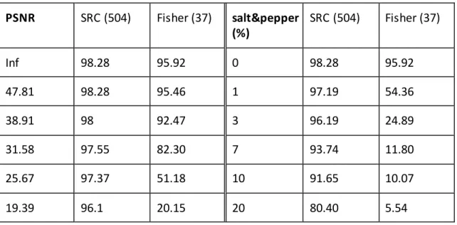
4.3.3 Noise 42
4.3.4 Illumination Compensation Capabilities 43
4.3.5 Geometric Distortion: shift, in-plane rotation and scaling 45 CHAPTER 5
GEOMETRIC NORMALIZATION AND BLOCK-BASED APPROACH 52
5.1 Geometric Normalization 52
5.2 Block Based Classification 59
5.2.1 Fusing Algorithms 61
CHAPTER 6
SRC WITH EMOTIONAL FACES 64
6.1 Classification of Emotional Faces via SRC 65
6.2 Description of the Database 65
6.3 Experiments 66
6.3.1 Emotion Classification 66
6.3.2 Action Units Identification 71
6.3.3 Identification Despite Emotions 74
CHAPTER 7
CONCLUSIONS AND FUTURE WORK 78 7.1 Conclusions and Future Work 78
REFERENCES 83
vii
LIST OF SYMBOLS
C number of classes classi a general class
M N
D dictionary
DictCoh coherence of the dictionary (D)
DictTestCoh mutual coherence between dictionary and test sample
i
m cardinality of classi
M M
S sparsifying matrix subjecti a general subject
SRC_miss number of samples mis-classified by the SRC algorithm M
x a coefficients’ vector
K M
X matrix of coefficients’ vector N
y a test sample, the signal under observation K
N
viii
LIST OF ABBREVIATIONS
2D two dimensional 3D three dimensional
ALM Augmented Lagrange Multiplier An Angry
AU Action Unit BP Basis Pursuit
CL Compressibility Level Co Contempt
CS Compressive Sensing or Compressive Sampling CF Cropped Faces
CFGN Cropped Faces with Geometric Normalization CMC Cumulative Match Count
DCT Discrete Cosine Transform DFS Distance from Face Space DFT Discrete Fourier Transform Di Disgust
DoG Difference of Gaussian DWT Discrete Wavelet Transform FACS Facial Action Coding System FRGC Face Recognition Grand Challenge
Fe Fear
FL Face Landmark
Ha Happy
HistEq Histogram Equalization IOD Inter Ocular Distance
LDA Linear Discriminant Analysis LOSO Leave One Subject Out
MCC Mean of the Class Coefficients MP Matching Pursuit
NC Normalization Coefficient OMP Orthogonal Matching Pursuit PCA Principal Component Analysis RankN Rank Normalization
ix Sa Sadness
SL Sparsity Level
SRC Sparse Representation-based Classifier Su Surprise
SVM Support Vector Machine
x
LIST OF FIGURES
Page
Figure 2.1 The synthesis or analysis problem 8
Figure 2.2 The synthesis or analysis problem (matrix wise) 9
Figure 2.3 Sparse versus compressible signals 11
Figure 2.4 L2 versus L1 balls 13
Figure 2.5 The cross-and-bouquet model for face recognition 18 Figure 3.1 Residuals of a correct classified test sample 31
Figure 3.2 Residuals of a misclassified test sample 31
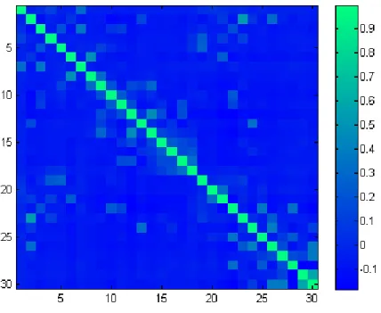
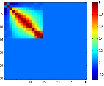
Figure 3.3 Correlation matrix of the 30 non-ordered coefficients of target class 33 Figure 3.4 Correlation matrix of the 30 coefficients of the target class ordered by
their algebraic values 33
Figure 3.5 Correlation matrix of the 30 coefficients of the target class ordered by
their absolute values 34
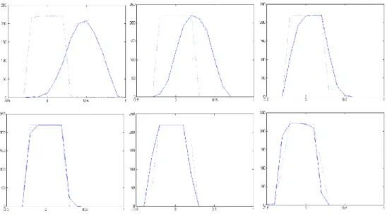
Figure 3.6 Histograms of target coefficients no.1, 2, 3, 4, 29, and 30 35
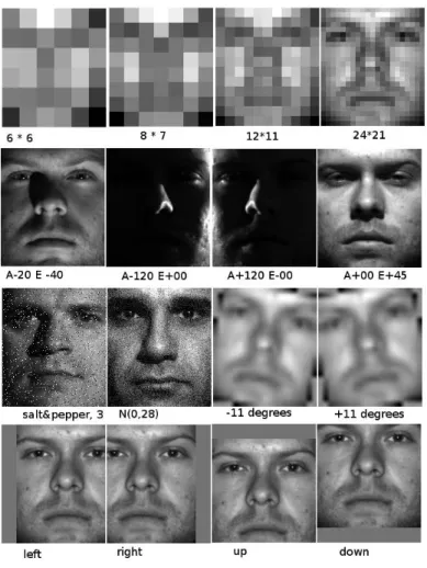
Figure 4.1 Elevation and azimuth angles 37
Figure 4.2 Samples of faces under adverse conditions 38 Figure4.3 Effects of the gallery size on classifiers’ performance 41 Figure 4.4 Performance (%) under Gaussian noise (plot of Table 4.2, left side) 43 Figure 4.5 Performance (%) under salt&pepper noise (plot Table 4.2, right side) 43 Figure 4.6 Effects of the shift geometric distortion (plot of Table 4.6, left side) 47 Figure 4.7 Effects of the rotation geometric distortion (plot of Table 4.6, center) 47 Figure 4.8 Effects of the zoom geometric distortion (plot of Table 4.6, right side) 48 Figure 5.1 An original and a cropped face in the CK+ database 53
Figure 5.2 Cropped Faces 53
Figure 5.3 Geometric normalization steps 54
Figure 5.4 Original and rotated face 54
Figure 5.5 Rotated and zoomed face 55
Figure 5.6 Photometric normalization 55
Figure 5.7 Aligned faces cropped with a fix size window 56 Figure 5.8 Aligned faces cropped with face landmarks 56 Figure 5.9 A face image partitioned into 2×2 and 3×3 blocks 59
Figure 5.10 Snapshot of a 3D dictionary 59
Figure 5.11 Conversion from a 3D to a 2D matrix of scores 60
Figure 5.12 Masks used for the fusing step 61
Figure 5.13 Rank based algorithm 63
xi
Figure 6.2 Emotional face with multiple AUs 72
Figure 6.3 CMC scores for AUs identification on the entire face 73 Figure 6.4 CMC scores at N+5 for AU identification. Bars left to right: whole face,
xii
LIST OF TABLES
Page
Table 2.1 Pseudo-code of DFS 20
Table 2.2 Pseudo-code of MCC 21
Table 2.3 Pseudo-code of biggest coefficient DFS 22
Table 2.4 Pseudo-code of three biggest coefficients DFS 23
Table 2.5 Pseudo-code of minimum LS norm 24
Table 2.6 Pseudo-code of different cardinality class DFS1 25 Table 2.7 Pseudo-code of different cardinality class DFS2 26
Table 2.8 Pseudo-code of MCC with absolute value 27
Table 4.1 Effects of down-sampling subspaces and image resolution on classifiers’
performance (%) 40
Table 4.2 Effects of the gallery size on classifiers’ performance 41 Table 4.3 Performance (%) under Gaussian (left) and salt&pepper noise (right) 42 Table 4.4 Training and test sets of experiments on illumination 44
Table 4.5 Illumination compensation capability 44
Table 4.6 Blind experiments on shift (left), rotation (centre), zoom (right) 47
Table 4.7 Blind experiment on shift 49
Table 4.8 Informed experiment on shift 50
Table 5.1 Performance of different experimental setups 57 Table 6.1 Confusion matrix of holistic SRC with CF (benchmark results) 69 Table 6.2 Confusion matrix of holistic SRC with CFGN (benchmark results 70 Table 6.3 Confusion matrix for 2×2 blocks based SRC on CF (benchmark results) 71
Table 6.4 Population of selected AUs 72
Table 6.5 Distribution of the number of subjects sharing emotion pairs 75 Table 6.6 Subject recognition rate (percentage) across expression 76 Table 6.7 Subject recognition rate (percentage) with a richer dictionary 77
xiii
ABSTRACT
ROBUST CLASSIFICATION BASED ON SPARSITY
Elena BATTINI SÖNMEZ
Computer Engineering Department PhD Thesis
Advisor: Assist. Prof. Dr. Songül ALBAYRAK
Classification is one of the most important problems in machine learning with a range of applications, including computer vision. Given training images from different classes, the problem is to find the class that a test sample belongs to. This thesis focuses on 2D face classification under adverse conditions . The problem is particularly hard in the presence of disturbances such as variations in illumination, expressions, pose, alignment, occlusion and resolution. Despite great interest in the past years, current pattern recognition methods still fail to classify faces in the presence of all types of variations. Recent developments in the theory of compressive sensing have inspired a sparsity based classification algorithm, which turns out to be very successful. This study investigates the potentialities of the Sparse Representation based Classifier (SRC) and, in parallel, it monitors the behaviour of some factors, which can reflect its performance. All experiments use the Extended Yale B and the Extended Cohn Kanade databases. The first dataset stores images with changes in illumination and has a cropped sub-directory of aligned faces, which allows for inserting a controlled amount of misalignment. The second database has coded action units and emotions, which permits to challenge both action units and emotion classification problems as well as the identity recognition despite emotions issue. Experimental results place SRC into the shortlist of the most successful classifiers mainly because of its inner robustness and simplicity.
Key Words: Classification, sparsity, face recognition, action unit, emotion, incoherence YILDIZ TECHNICAL UNIVERSITY GRADUATE SCHOOL OF NATURAL AND APPLIED SCIENCES
xiv
ÖZET
SEYREKLİĞE DAYALI GÜRBÜZ SINIFLAYICI
Elena BATTINI SÖNMEZ
Bilgisayar Mühendisliği Bölümü Doktora Tezi
Tez Danışmanı: Yrd. Doç. Dr. Songül ALBAYRAK
Bilgisayarla görmenin de içinde olduğu farklı uygulamalarda kullanılan sınıflama konusu makine öğrenmesindeki en önemli problemlerden biridir. Sınıflama, farklı sınıflara ait eğitim örneklerinin sisteme verilerek test örneğinin hangi sınıfa ait olduğunun bulunması problemidir. Bu tez çalışmasında aydınlatma farklılıkları, yüz ifadesi, poz, yanlış hizalama ve çözünürlük gibi bozucu etkiler altında 2B yüz sınıflama problemine odaklandık. Son yıllarda yüz tanıma konusuna çok büyük bir ilgi olmasına karşın, mevcut örüntü tanıma metodları tüm bu bozucu etkilerin var olduğu durumlarda yüz sınıflamada başarısız olmaktadır. Sıkıştırmalı algılama teorisinde görülen gelişmeler, seyreklik tabanlı sınıflayıcılara doğru yayılmış ve başarılı sonuçlar alınmıştır. Bu çalışmada seyrek yaklaşım tabanlı sınıflama algoritmasının potansiyeli ve başarımı nı etkileyen faktörlere karşı davranışı araştırılmıştır. Çalışmada gerçekleştirilen tüm deneylerde Exteded Yale B ve Extended Cohn Kanade veritabanları kullanılmıştır. Birincisinde aydınlatma farklılıkları olan görüntüler kontrol edilebilir miktarda hizalamaya izin verecek şekilde kırpılarak alt dizinlere yerleştirilmiştir, eylem birini ve yüzdeki duygunun kodlandığı ikinci veritabanı sınıflama problemi kadar yüz ifadesine rağmen kişi tanımaya da uygundur. Deneylerdeki sonuçlar SRC'yi, başta gürbüzlüğü ve basitliğinden dolayı en başarılı sınıflandırıcılar listesine sokmuştur.
Anahtar Kelimeler: Sınıflama, seyreklik, yüz tanıma, eylem birini, duygu, uyumsuzluk YILDIZ TEKNİK ÜNİVERSİTESİ FEN BİLİMLERİ ENSTİTÜSÜ
1
CHAPTER 1
INTRODUCTION
1.1 Literature Review
Automatic identification and verification of humans using facial information has been one of the most active research areas in computer vision. The interest on face recognition is fuelled by the identification requirements for access control and for surveillance tasks, whether as a means to increase work efficiency and/or for security reasons. Face recognition is also seen as an important part of next-generation s mart environments [1], [2].
Face recognition algorithms under controlled conditions have achieved reasonably high levels of accuracy. However, unde r non-ideal, uncontrolled conditions, as often occur in real life, their performance becomes poor. Their main handicaps are the changes in face appearances caused by such factors as occlusion, illumination, expression, misalignment, pose, make-ups and aging. In fact the intra-individual face differences due to some of these disturbances can easily be larger than the inter-individual variability [3], [4], [5].
We briefly point out below some of the main roadblocks to wide scale deployment of reliable face biometry technology.
Effects of Illumination: changes in illumination can vary the overall magnitude of the
light intensity reflected back from an object and modify the pattern of shading and shadows visible in an image [5]. It was shown that varying illumination is the most detrimental to both human and machine accuracies in recognizing faces. It suffices to quote simply the fact that in the Face Recognition Grand Challenge (FRGC) the 17
2
algorithms competing in the controlled illumination track have achieved a median verification rate of 0.91 while in contrast, the 7 algorithms competing in the uncontrolled illumination experiment have achieved a median verification rate of only 0.42 (both figures at a false acceptance rate of 0.001). The difficulties posed by variable illumination conditions, therefore, remain still one of the main roadblocks to reliable face recognition systems.
Effects of Expression: Facial expression is known to affect the face recognition
accuracy though in the current literature, a full-fledged analysis of the deterioration caused by expressions has not been documented. Instead, most studies either focus on expression recognition alone or on face identification alone. It is quite interesting that this dichotomy is also encountered in bi ological vision. There is strong evidence that facial identity and expression might be processed by separate systems in the brain, or at best they are loosely linked [6]. To state the same concept in a different way, faces with emotions present two interesting and concomitant problems:
The first one is automatic understanding of the mental and emotional state of the subject, as reflected on the facial expression. It is stated that about 55% of interpersonal feelings and attitudes, such as like and dislike, can beconveyed via facial expressions. In other words, the human face is a rich source of non-verbal information providing clues to understand social feelings and facilitating the interpretation of intended messages.
The second problem is the identity recognition based on emotional faces. The plethora of publications on face biometry has indicated that the face remains the holy grail of biometric recognition. Unfortunately, while face enables remote biometry, it is handicapped by several factors among which there is the presence of expressions, [7].
Effects of Misalignment: Real-world images have faces with background, which
requires the use of face detectors to locate and crop the face before being able to classify it. In other words, in an automatic face recognition system, face detection and cropping are necessary pre-processing steps and its final recognition rate heavily relies on their accuracies. At the current state of the art, automatic cropping or even manual
3
face cropping may result in big misalignments, such as faces with translation, rotation and scaling, which, in turn, decrease the success rate of the face recognition system. In 2005 Gong et al. [8] proposed a new algorithm to increase the robustness of the classical Gabor features to misalignment, in 2009 Wagner et al. [9] introduced an iterative sparse classifier, which is robust to shifts and rotations, in 2010, the same problem is faced by Yan et al. [10] who proposed a general L1 norm minimization formulation. Nevertheless, bad cropping and misalignment are still among the main factors impeding accurate face recognition.
Effects of Pose: Facial pose or viewing angle is a major impediment to machine-based
face recognition. As the camera pose changes, the appearance of the face changes due to projective deformation (causing stretching and foreshortening of different part of face); also self-occlusions and/or uncovering of face parts can arise, [11]. The resulting effect is that image-level differences between two views of the same face are much larger than those between two different faces viewed at the same angle. While machines fail badly in face recognition under viewing angle changes, that is, when trained on a gallery of a given pose and tested with a probe of set of a different viewing angle, humans have no difficulty in recognizing faces at arbitrary poses. It has been reported in [11] that the performance of Principal Component Analysis (PCA) based method decreases dramatically beyond 32 degree yaw and those for Linear Discriminant Analysis (LDA) beyond 17 degree rotation.
Effects of Occlusion: The face may be occluded by facial accessories such as
sunglasses, a snow cap, a scarf, by facial hair or other paraphernalia. Furthermore, the subjects in an effort to eschew being identified can purposefully cover parts of their face. Although it is very difficult to systematically experiment with all sorts of natural or intentional occlusions, results reported in [11] show that methods like PCA and LDA fail quite badly (e.g., sunglasses and scarf scenes in AR database). Recent work on recognition by parts shows that methods that rely on local information, can perform fairly well under occlusion [12], [13], [14].
Effects of Low Resolution: The performance loss of face recognition with decreasing
resolution is well known and documented, [15]. For example, 30 percentage point drops are reported in [15] as the resolution changes from 65×65 to 32×32 pixel faces.
4
The robustness to varying resolution becomes relevant especially in uncontrolled environments where the face may be captured by a security camera at various distances within its field of view.
In recent years the growing attention in the study of the compressive sensing theory fuelled an increase interest in the sparse representation of signals which has suggested a different approach to achieve robust classification. The basic idea is to cast classification as a sparse representation problem, utilizing new mathematical tools from the compressive sampling studies [16], [17], [18]. The new algorithm was first introduced by Wright et al. in [14]; it proposes a new classification technique called Sparse Representation-based Classifier (SRC) because based on the sparse representation of the test sample. The novelty of this algorithm is in the classification method, which uses the coefficient vector, ,x returned by a synthesis algorithm claiming that x has enough discriminative power to classify the current test sample. It is important to point out that, instead of the classical dictionaries, such as Fourier, DCT, or Wavelets, Wright et al. used an ad-hoc dictionary, D , built by aligning, column after column, the down-sampled training images themselves. The main idea underlying this approach is that, if sufficient training samples are available for each class, then it is possible to represent every test sample as a linear combination of just those training samples belonging to the same class. Seeking the sparsest representation automatically discriminates between the various classes present in the training database and also provides a simple and effective mechanism for rejecting outliers, invalid test samples not belonging to any class of the training set. SRC method was inspired by the compressive sensing theory and it works very well even if, at first glance, it violates some of its important requirements. One of the aims of this study is to distinguish among the relevant and the irrelevant requirements of SRC.
1.2 Aims of the Thesis
The aim of this work is to explore the capabilities of the sparse representation based classifier (SRC). In order to do that, we tackled different classification issues using two databases of faces; that is, we worked on identity recognition with faces corrupted by
5
noise, geometric distortions or illumination changes, as well as we challenged the emotion and action unit identification problems and we studied the deterioration caused by expressions on the identity recognition task with emotional faces. While running all experiments, we monitored different parameters considered critical for the performance of SRC, such as the sparsity level (SL) of the coefficients’ vector and the level of incoherence of the dictionary (DictCoh) so as to detect “if” and “how” those measurements are really correlated to the performance of SRC, and we introduced other critical parameters capable of predict the success rate of SRC. Moreover, we made statistical studies on the correlation matrix of the target coefficients and on the distribution of the coefficients vector with the aim to understand and justify the performance of SRC. Finally, for some critical experiments, we improved the original success rate of SRC by enlarging its dictionary, using a block-based approach or pre-processing all samples with geometric normalization.
Chapter 2 gives a general overview of the sparse representation and compressive sensing theory, followed by an introduction of the sparse representation based classifier (SRC), with a case study on face recognition. Chapter 3 introduces some parameters, which are considered critical for the performance of SRC, it proposes new important measurements related to its success rate, and it stores the results of statistical studies on the distribution of the coefficients’ vector and their correlation matrix. Chapters 4, 5 and 6 are empirical chapters. The aim of all experiments is to test the robustness of the sparse classifier to adverse conditions, to identify the critical parameters correlated to the performance of SRC, and to explore possible variations. More in detail, Chapter 4 works with a database of clean aligned and cropped faces affected by changes in illumination. This database naturally allows us to study the robustness of SRC to illumination changes as well as it permits to insert a controlled amount of shit-rotation-zoom or unwanted information and to run experiments on in-plane geometric distortion and noise. For some relevant cases, Chapter 4 monitors also the critical parameters given in Chapter 3; some of the experiments documented in Chapter 4 were previously presented in [19] and [20]. Chapter 5 details the geometric normalization pre-processing technique together with the block based
6
approach. Chapter 6 works with a database of coded emotional faces, it presents experimental results on emotion and action unit identifications as well as it investigates the deterioration caused by the presence of expressions in the identity recognition task. Conclusions are drawn in Chapter 7.
All experiments were run in the MATLAB R2007b environment on different platforms.
1.3 Hypothesis
We want to prove the conjecture that sparse representation enables the creation of templates robust against various factors impeding accurate face recognition such as illumination, expression, misalignment, and noise. We demonstrate, experimentally, the robustness of the SRC classifier under adverse conditions. Important to notice that the idea of the SRC algorithm was inspired by the compressive sensing (CS) theory, but then, on the practical side, SRC violates the fundamental theoretical assumption of CS such as the restricted isometry property (RIP), which is measured as the level of incoherence of the dictionary. Nevertheless, it is a very successful classification method, inherently robust due to the presence of the L1 norm. This study points out the differences between CS and SRC, and conjectures that compressibility is the only pre-requisite necessary for successful classification.
7
CHAPTER 2
THE SPARSE REPRESENTATION BASED CLASSIFIER (SRC)
2.1 Sparse Representation of Signals
A sparse representation of signals allows for a high level representation of the data, which is both the most natural and insightful one. In the signal processing community, looking for a compact representation of the data is equivalent to search for a n orthogonal transformation where the signal can be represented, in the new domain, as a superposition of few basic elements or atoms; classical examples of such a basis are Discrete Fourier Transform (DFT) with its variation Discrete Cosine Transform (DCT), and the Discrete Wavelet Transform (DWT). The usual approach is to choose one orthogonal basis and use it to represent signals, because the basis is a standard one, the transformation does not consider the particularities of the signals.
A more recent approach rejects orthogonality and standard basis on behalf of over-complete dictionaries. A dictionary, D, is a collection of parameterized waveforms
where each waveform, di, is a discrete time signal of length N called atom and it has unit length, ||di|| 1. Dictionaries are complete, if they contain exactly N linearly independent atoms, and over-complete, if they contain more than N atoms; Dis an over-complete dictionary. The use of over-complete dictionaries allows a sparse representation because we can decompose the target signal in more than one ways; moreover, the non unique representation of the observed signal gives the possibility of adaptation, the potential of choosing among many representations the one which is most suited to our purpose. Some of the goals are:
8
Sparsity: we want to obtain the sparsest possible representation of the object, i.e. the
one with the fewest significant coefficients. This is why sparse representation helps to capture higher order correlations in the data, it allows for the extraction of a categorically or physically meaningful solution, it gives a parsimonious representation of the signal and, finally, it is easily coupled with dictionary learning techniques.
Discriminative power: the algorithm must produce a good separation of the observed
signals Y= [y1,..., yk] into classes.
Robustness: small perturbation on ,y || y||, should not seriously degrade the results; that is, a small perturbation in the observed data should gender a commensurate perturbation in the solution, || x||. Robustness is guaranteed by a particular structure imposed to the dictionary called Restricted Isometry Property (RIP) or incoherence (detail information will be given shortly).
Following the standard notation, the matrix format of the general reconstruction or projection step is:
x D
y (2.1)
where D N M is the dictionary, N
y the observed signal, and x M is the coefficient vector.
The following picture gives the graphical representation of the problem:
9
When stacking together more than one signal, equation (2.1) becomes: X
D
Y (2.2)
where N K
Y and M K
X , as depicted by the following picture:
Figure 2.2 The synthesis or analysis problem (matrix wise)
2.1.1 Synthesis versus Analysis
From the synthesis point of view, equation (2.1) has infinitely many solutions at every point; among all possible solutions, we are interested in the one that minimizes the error and has the minimum number of non-zero elements; in other words, we want to minimize the following quantity:
0 2 || || ||
||y D x x (2.3)
where || x||0 is the L0 norm, it is simply the count of non-zero elements.
More in details, considering column “j” of matrix Y, yi, during the synthesis step, we
need to determine the “best” coefficients along column “j” of X, to decompose signal yj, j 1 , ,K, such that: M i j i i j d x y 1 , (2.4)
or to approximate it using only “t” atoms: t t i j i i j dx R y 1 , (2.5)
10
On the contrary, from the analysis point of view, we are interested in determining a "good" projection matrix, D, capable of down-sampling the original signal M
x into y N, N M, without losing critical information.
It is important to notice that synthesis is the operation of building up a signal by superposing atoms, it is the reconstruction step implemented using Basis Pursuit [21] or similar algorithms, while analysis is the projection operator; that is, also the analysis step involves the task of associating coefficients to atoms for any given signal. However, the synthesis and analysis operators are very different because D is a flat matrix, it is not invertible, and the synthesis step cannot use the same coefficients of the analysis step. That is, synthesis and analysis are not self-adjoint operators. Compressive sensing theory is concerned with both the analysis and the synthesis steps, while the Sparse Representation based Classifier (SRC) is strictly related to the synthesis step.
2.1.2 Compressive Sensing Theory
Compressive sensing or compressive sampling (CS) [16], [17], [18] is a novel sensing-sampling paradigm that goes against the common wisdom in data acquisition. CS theory exploits the fact that many natural signals are sparse or compressible in the sense that they have a concise representation when expressed in a proper base; it asserts that it is possible to desire efficient sampling protocols that capture the useful information content embedded in a sparse signal and condense it in a small amount of data.
The actual data acquisition systems, like the one used in the digital camera, follow the Shannon/Nyquist sampling theorem, which tells us that, when uniformly sampling a signal, we must sample at least two times faster than its bandwidth; as a result, we end up with too many samples which are then compressed before being stored or transmitted. More in details, following the Shannon/Nyquist sampling theorem, current data acquisition systems (1) acquire the full M-sample signal ,x (2) they compute the complete set of transform coefficients, (3) they locate the s-largest
11
coefficients and discard the (M s) smallest ones, and (4) they encode the s couples (value, location) of the largest coefficients. As an alternative, the compressive sensing theory proposes a more general data acquisition approach that condenses the signal directly into a compressed representation without going through the intermediate stage of taking all samples. That is, CS theory proposes a new sampling process and asserts that it is possible to recover sparse or compressible signals from far fewer samples than traditional methods use.
Informally, we may state that CS is concerned with s-sparse or s-compressible signals and we may define a signal x as sparse if all of its entries are zeros except few spikes , and a signal x as compressible if its sorted coordinates decay rapidly to zero. The following picture gives a graphical representation of sparse and compressible signals in
3 :
Figure 2.3 Sparse versus compressible signals (courtesy of Boufounos et al. [22]) During the sampling step, to ensure a lossless mapping, it is necessary to impose strong assumptions on the structure of the dictionary D, which must preserve the distance between any two s-sparse vectors; mathematically speaking it must have the Restricted Isometry Property (RIP) of order 2s where sis the level of sparsity of the signal. In formula: 2 2 2 2 2 2 2 2 2 )|| || || || (1 )|| || 1 ( s x D s x s x (2.6)
where 2s is the restricted isometry constant; in other words, matrix D with the RIP of
order 2s projects into the down-sampling subspace by preserving information of any s-sparse vector. The RIP property can be verified using the level of incoherence of the dictionary in use: compressive sensing theory states that it is desirable to work with an
12
incoherent matrix, where the coherence parameter of the dictionary D is defined as follows: | , | max ) (D i j di dj DictCoh (2.7)
In other words the coherence is the cosine of the acute angle between the closest pair of atoms. Informally, we may say that a matrix is incoherent if DictCoh(D) is small, which is equivalent to say that all atoms of D are very different from each others, they are (nearly) orthogonal vectors.
Moreover, atoms of dictionary D must be incoherent with the basis, S M M, in
which x M is assumed to be sparse. That is, in equation (2.1) the original waveform, x is assumed to be already sparse, when this does not happen, the , compressive sensing theory requires the use of a sparsifying matrix, S M M, and the system to be solved becomes:
z S D
y , where x S z (2.8)
obviously x M and z M are the same waveforms from different points of view, but the signal z is sparse.
The incoherence of N M
D and M M
S means that the information carried by the few entries of M
z is spread all over the N entries of y N, that is, each
sample yi is likely to contain a piece of information of each significant entry of zi. These properties allow for a non adaptive sampling step, a measurement process which does not depend to the length of x M, and produce democratic measurements, meaning that every dimension carries the same amount of information, and, therefore, they are equally (un)important.
During the reconstruction step, theoretically, the sparsest solution of system (2.1) can be obtained by solving it as a non-convex constrained optimization method, (2.3), practically this solution is infeasible because it requires an exhaustive enumeration of all
s M
13
Compressive sensing theory showed that, under certain sparsity conditions [23] the convex version of this optimization criterion yields exactly to the same solution. The reason for that is in the geometric shape of the L1 ball, which is represented together with the L2 ball in the following picture:
Figure 2.4 L2 versus L1 balls (courtesy of Baraniuk [16])
In Figure 2.4 the green plane is the null space of dictionary D (defined in Paragraph 2.1.3), S^ is the wrong solution recovered by the L2 norm and S S
^
is the correct solution recovered by the L1 norm. That is, knowing that any s-sparse vector lays on an s-dimensional hyper-plane close to the coordinate axes, and that we do search for a solution by blowing the interesting balls as far as its border points touch the null space of D, the geometrical shape of the L1 ball, which is pointing along the coordinate axes, allows for perfect recovery of any s-sparse or s-compressible signals, while the L2 ball fails.
Therefore, when the signal to be recovered is sparse enough, compressive sensing theory state that instead of (2.3) we obtain the same solution by solving a much easier convex version:
1 2 || || ||
|| y D x x (2.9)
Where || x||1 is the L1 norm, equal to the sums of the absolute values of all coefficients.
14
Interesting to point out that the RIP, or incoherence, property is necessary during the analysis or projection step while during the synthesis step it is the level of sparsity of the wanted solution, which allow for a perfect reconstruction; experimental results proved that the resulting coefficient vector has discriminative power, and, that its sparsity level affects the success rate of the sparse classifier. That is, the idea of using a sparse classifier was born as a possible application of the emerging theory of compressive sensing but, because it is related only to the synthesis step, it does not have the same constraints.
2.1.3 Under vs Over-Determined System of Equations
Let us consider Equation (2.1) y D x, with D N M, from the linear algebra point of view:
1. If N=M, Equation (2.1) is a standard linear system and the solution is unique if D has full rank, which is equivalent to say that the determinant(D)≠0; the unique solution is the minimum norm solution.
2. If N<M, D is a flat matrix having more variables-columns than equations-constraints-rows; the over-complete frame generates an under-determined system of equation. If the equations are inconsistent the system has no solution, otherwise there is an infinitive number of solutions. In the second case, we have a General Minimum Norm Problem, that is, among all infinitely many solutions, we are interested in the one minimizing some norms; in case of L2 norm we have the classical Minimum Norm Problem, in case of L0 norm, we are looking for the sparsest solution, the one with the minimum number of non-zero coefficients. That is, a flat matrix has a null space, NSD {v:D v 0} of dimension (M N), and if
x D
y holds also y D (x v) will hold, for all vectors v NSD; obviously the true solution is the sparsest one. CS theory proved that, when x is enough sparse, the minimum L0 and the minimum L1 norms return the same solution.
3. If N>M matrix D is tall, it has more equations-constraints-rows than variables-columns, and Equation (2.1) has generally no solution. In this case, we are interested in finding x which minimizes the quantity || y D x||2, and this is the
15
Standard Least Square Problem, due to the presence of the L2 norm; if, among all possible approximations, we are looking for the one minimizing some norms, then we have a General Minimum Norm Standard Least Square Problem. Again, the Minimum Norm Least Square problem looks for the coefficient vector x with minimum L2 norm, while we are now interested in the sparsest solution, the one having minimum L0 norm.
Notice that in case of face recognition, N is the resolution of the image while M is the gallery size, the total number of training samples; depending to the experiment under investigation, all cases are possible, but points 2 and 3 are more common, and in both circumstances, we have a general minimum norm problem. Moreover, because columns of D are vectorized faces, and different faces of the same subjects are linearly independent, matrix D has always full rank.
From an algorithmic point of view, when looking for the coefficient vector x having minimum L2 norm, we may use either the pseudo-inverse or the QR factorization of dictionary D ; but if we are looking for the coefficient vector x having minimum L1 norm, then we need a synthesis algorithm, such as LASSO [24], OMP [25], Augmented Lagrange Multiplier [26], etc. Imposing the minimum L2 norm has a number of computational advantages but it does not provide sparse solutions as it has the tendency to spread the energy among a large number of entries of x instead of concentrate on few coefficients; on the contrary, the minimum L1 norm naturally selects the few and high correlated column of D , and, because of this, the resulting coefficients vector is sparse and has discriminative power.
2.1.4 Synthesis Algorithms
Sparse recovery algorithms reconstruct sparse signals from a small set of non-adaptive and democratic linear measurements. Given y N, the measurement vector belonging to a low dimensional space, and the synthesis matrix D N M, N M.
The goal is to reconstruct x M, the original signal belonging to a high dimensional space, knowing that x is sparse. In other words, the goal is to obtain a sparse
16
decomposition of a signal x with respect to a given dictionary D and the measurements vector y When we allow for some disturbance elements, we can . represent the system with the following formula:
1 || ||
minx x such that || y D x||2 (2.10)
where ε is a little value. The ideal optimum recovery algorithm needs:
to be fast: it should be possible to obtain a representation in the order of (N) or at most (Nlog(N)) time;
to require minimum memory storage;
to provide uniform guarantees: the algorithm must recover all sparse signals, with high probability;
to be stable: small perturbations of y do not seriously degrade the results.
There are two distinct major approaches to sparse recovery, both of them with pros and cons. The first approach uses greedy methods to compute the support of the signal iteratively. This type of algorithms is usually fast but they do not provide strong guarantees of convergence; examples are Orthogonal Matching Pursuit (OMP) [25] and Matching Pursuit (MP) [27]. The second approach is to cast the sparse recovery problem into a linear programming one; that is, to solve (2.9) instead of (2.3). These methods provide guarantees of convergence and stability, but their running time is not polynomially bounded; examples are Basis Pursuit (BP) [21], and LASSO [24]. A comprehensive review of five representative L1-minimization methods can be found in [26]. Recent developments of the CS theory increased the interest in L1 reconstruction methods and produced new algorithms such as “Compressive Sampling Matching Pursuit” (CoSaMP) in [28], and “A* Orthogonal Matching Pursuit: Best-First Search for Compressed Sensing Signal Recovery” (A*OMP) in [29], with the aim to bridge the gap between the previous two approaches.
2.2 Sparse Representation based Classifier
From a synthesis point of view, the under-determined system (2.1) is used to model different problems where only a small number of information is available out of a very
17
large set of possible sources. Among all possible solutions the sparsest one is preferred because it stores a high description of the data and, therefore, it is useful for the feature extraction stage, or concept generation stage, of pattern recognition problems. Other applications include data compression, high-resolution spectral estimation, direction-of-arrival estimation, speech coding, and function approximation.
The main idea is that many interesting phenomena in nature lie in a smaller, often much smaller, dimensional subspace as compared to the observed signal dimensionality; in other words, the intrinsic magnitude of a signal subspace, where all the variations of the signal occur, is significantly smaller than the ambient di mension. Sparse approximation methods attempt to discover this subspace, and to represent events and objects in that subspace.
Identity recognition is a good case in point: it is assumed that a face can be represented as a sparse linear combination of training samples, which are alternate images of the same subject, and that the resulting combiner coefficients contain discriminative information. Assuming that all training samples of a single class lie on the same subspace, a new down-sampled test image y of classi, yi, will lie in the
linear span of its class’s training samples and, therefore, can be represented as a linear combination of only the atoms of Di, that is:
i x D
y (2.11)
where xi is a coefficient vectors having all zero entries except for the coefficients of
classi, xi = [0,,0,x1,,xmi,0,,0]
T
; if-when the number of different classes is sufficiently large the representation of y is naturally sparse.
Interesting to notice that the sparse representation based classifier allows for an ad-hoc solution to deal with errors and occlusions. That is, in real world applications the test image, ,y could be partially corrupted or occluded, in this case, Equation (2.1) should be modified as:
e x D
18
where N
e is the error, which is assumed to be sparse, but, the location of non zeros entries is unknown and, obviously, different in every test image. In this case, the simple solution proposed by Wright et al. [14] and [30] is to use an expanded dictionary, '
D =[D |I]; that is, the original dictionary N M
D is expanded to size )
(N M N
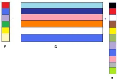
by concatenating a coherent part D of faces to a non-coherent part implemented by the identity matrix, I N N. The use of such an expanded dictionary totally changes the geometry of the system, which was dubbed as cross-and-bouquet (CAB) in [30], due to the fact that the columns of the identity matrix are highly incoherent, they span a cross polytope which captures the error, whereas the columns of D are tightly clustered like a bouquet of flowers. The geometric representation of the expanded dictionary D', built as concatenation of sub-dictionaries, is illustrated in Figure 2.5:
Figure 2.5 The cross-and-bouquet model for face recognition
In other words, the N dimensions of the polytope represent the incoherent noise while the tight bundle captures faces and expressions. This configuration achieves image source separation between face and noise sources.
19
2.2.1 A case study: Sparse Representation for Face Recognition
The plethora of face recognition methods can be categorized under template-based and geometry-based paradigms. In the template-based paradigm one computes the correlation between a face and one or more model templates for face identity. Methods such as Principal Component Analysis (PCA), Linear Discriminant Analysis, Kernel Methods, and Neural Networks as well as the statistical tools such as Support Vector Machines (SVM) can be put under this category [11], [31]. In the geometry-based paradigm one analyses explicit local facial features and their configurational relationships. The SRC method can be interpreted as a non-linear template matching method.
From a practical point of view, when SRC is applied to face recognition the general framework is as follows: assuming that the database stores mi faces of subjecti, the
column matrix Di= [
i m d d
d1, 2,, ] aligns, column after column, the mi training
samples of classi; where di is a down sampled training face. Having C classes, the
synthesis dictionary D must concatenate all training samples of all classes, that is, D= [D1,D2,,DC]
M N
with M m1 mC, and the problem is modelled as in Equation (2.1), where y is the face to be classified, and x the vector of coefficients to be computed.
It is interesting to point out that, when working with images, dictionary D is not always flat because the gallery size, which is the total number of training samples, maybe less than the required resolution. Moreover dictionary D may not be incoherent, because it is made up of faces, which are not orthogonal vectors. Nevertheless the performance of SRC is very good, as shown in Chapters 4 and 6.
20
2.2.2 Algorithms
From an algorithmic point of view the sparse representation based classifier can be implemented in different ways, all variations working on the coefficient vector, x returned by a synthesis algorithm.
The framework is the one introduced in Paragraph 2.1 with C classes, a dictionary D of size N M, where N is the resolution of the image and M m1 mC is the total number of training samples, and x [0,,0,x1,,xmi,0,,0] is the coefficient
vector x restricted to the entries of classi.
During this study, we tried different variations of SRC, some of them presented in the rest of this paragraph.
Distance from Face Space (DFS)
Wright et al. [14] proposed the Distance from Face Space (DFS) variation defined as follows: 2 || || min ) (y i y D xi Class (2.13)
That is, the class assigned to the test sample y is the one producing minimum residual error, when the face is reconstructed from the class coefficients found by the solution of (2.10). The following table gives the pseudo-code of DFS:
Table 2.1 Pseudo-code of DFS
INPUTS: a dictionary D , and an observed signal y to be classified CODE:
1. Normalize all columns of D and the test sample y by imposing unit L2 norm 2. Solve the L1 minimization problem:
1 || ||
minx x such that || y D x||2
3. Compute the residuals, resi || y D xi ||2 i 1,,C
21
Mean of the Class Coefficients (MCC)
The second approach, proposed in this work, is called Mean of the Class Coefficients (MCC) and it is defined simply as:
)) ( ( max ) (y i E xi Class (2.14)
Notice that MCC simply calculates the average of the class coefficients and assigns to the test sample y the class having the maximum mean.
The following table gives the pseudo-code of MCC:
Table 2.2 Pseudo-code of MCC
INPUTS: a dictionary D , and an observed signal y to be classified CODE:
1. Normalize all columns of D and the test sample y by imposing unit L2 norm 2. Solve the L1 minimization problem:
1 || ||
minx x such that || y D x||2
3. Compute the mean of the class’s coefficients, mean(xi), i 1,,C
22
Biggest Coefficient DFS
The idea underlying this variation is to consider as decision statistic the biggest coefficient for every class. This is based on the study of the coefficient’s distribution (Paragraph 3.2.2) where we point out that the histogram of the biggest coefficient has the least overlap as compared to those of smaller coefficients.
Table 2.3 Pseudo-code of biggest coefficient DFS
INPUTS: a dictionary D , and an observed signal y to be classified CODE:
1. Normalize all columns of D and the test sample y by imposing unit L2 norm 2. Solve the L1 minimization problem:
3. minx ||x||1such that || y D x||2
Select the biggest coefficient out of every class: bi max(xi), i 1,,C 4. Compute the residuals, resi || y D bi ||2, i 1,,C
23
Three Biggest Coefficients DFS
This variation is a modification of the previous one, still based on the results of Paragraph 3.2.2; it assumes that the top three coefficients of every class store enough discriminative power and makes classification considering only those coefficients.
Table 2.4 Pseudo-code of three biggest coefficients DFS
INPUTS: a dictionary D , and an observed signal y to be classified CODE:
1. Normalize all columns of D and the test sample y by imposing unit L2 norm 2. Solve the L1 minimization problem:
3. minx||x||1 such that || y D x||2
Select the 3 biggest coefficient out of every class: 3bi top3(xi), i 1,,C 4. Compute the residuals, resi || y D 3bi||2, i 1,,C
24
Minimum LS Norm
This variation was suggested by [32]; the idea is to solve the usual system y D x looking for the minimum L2 norm; that is, instead of using a synthesis algorithm, we calculated the coefficient vector x using either the pinv(D) or the QR factorization of dictionary D ; obviously, in both cases, the solution will not be sparse because the minimum L2 norm has the tendency to spread the energy among a large number of entries of x instead of concentrate on few coefficients. We tested the “Minimum LS norm” variation for the emotion classification experiment, but our results were always much worse than the ones presented in Paragraph 6.3.1. Important to point out that also Wright et al. in [14] make a comparison between DFS and the “Minimum LS norm” and show the superior performance of DFS.
Table 2.5 Pseudo-code of minimum LS norm
INPUTS: a dictionary D , and an observed signal y to be classified CODE:
1. Normalize all columns of D and the test sample y by imposing unit L2 norm 2. Solve the L2 minimization problem:
2 || ||
minx x such that || y D x||2
3. Compute the residuals, resi || y D xi ||2 i 1,,C
25
Different Cardinality Class DFS1
This variation was suggested by the idea that the performance of DFS can be affected by the different cardinalities of the classes. This version of DFS considers only the top "min_card" coefficients of every class, where "min_card" is the minimum of the number of representatives among all the C classes. In pseudo-code:
Table 2.6 Pseudo-code of different cardinality class DFS1
INPUTS: a dictionary D divided into classes of cardinality (card1,…, cardC), and an
observed signal y to be classified
CODE:
1. Normalize all columns of D and the test sample y by imposing unit L2 norm 2. Solve the L1 minimization problem:
1 || ||
minx x such that || y D x||2
3. min_card=min(card1,…, cardC), ti= top “min_card” coefficients of xi, i: 1, ,C
4. Compute the residuals: resi || y D ti ||2 i 1,,C
26
Different Cardinality Class DFS2
This variation was created with the aim to increase the robustness of DFS in case of classes with different cardinality. It multiplies the DFS score by a normalization coefficient, in pseudo-code:
Table 2.7 Pseudo-code of different cardinality class DFS2
INPUTS: a dictionary D divided into classes of cardinality (card1,…, cardC), and an
observed signal y to be classified
CODE:
1. Normalize all columns of D and the test sample y by imposing unit L2 norm 2. Solve the L1 minimization problem:
1 || ||
minx x such that || y D x||2
3. Compute the residuals: resi || y D xi ||2 i 1,,C
4. norm_coeff=(dim(x)-cardi)/ dim(x); scorei= norm_coeff × resi, i: 1, ,C
OUTPUT: Class(y) = the class producing minimum score
Nearest subspace SRC
In this variation the DFS algorithm is applied separately to every subspace. In case of the emotion classification challenge every test subject will have 7 dictionaries, one per emotion, with different cardinality depending to the total number and the type of emotional faces of the current test subject. Instead of putting all these dictionaries together, D=[AnDict, CoDict, DiDict, FeDict, HaDict, SaDict, SuDict], and solve the system y D x, we do now solve 7 separate systems.
Obviously, all coefficient vectors are NOT sparse any more neither with a synthesis algorithm, because, at any time, the dictionary stores only one class; classification is done as usual by assigning the test sample to the nearby class.
27
Variation2: it solves the 7 systems separately by imposing minimum L2 norm. Both variations were tested in the emotion classification experiments; in both cases the obtained performance is worse than the one documented in Chapter 6.
MCC with Absolute Value
The MCC variation previously introduced has a very good performance but it lacks from mathematical background; by introducing the absolute value, the algorithm calculates the mean of the L1 norm of the class’s coefficients, but this variation is not as successful as the original MCC.
Table 2.8 Pseudo-code of MCC with absolute value
INPUTS: a dictionary D , and an observed signal y to be classified CODE:
1. Normalize all columns of D and the test sample y by imposing unit L2 norm 2. Solve the L1 minimization problem:
1 || ||
minx x such that || y D x||2
3. Computer the mean of the class’s coefficients, mean(abs(xi)), i 1,,C
OUTPUT: Class(y) = the class having maximum average
The most successful variations are DFS and MCC, their performance is generally the same; for this reason, in the sequel, we will refer to them in the tables simply as SRC.
28
CHAPTER 3
STUDY OF THE CHARACTERISTICS OF SRC
In this chapter we present some parameters, which are considered critical for the performance of the sparse representation based classifier, and we introduce other new critical parameters. In Chapter 4, for some relevant experiments, we will monitor those measurements with the aim to determine “if” and “how” they are correlated to the success rate of SRC. Furthermore, this chapter runs experiments to investigate some statistical properties of the coefficients’ vector. All experiments are based on a particular selection done on the cropped sub-directory [33] of the Extended Yale B database [34]: 38 subjects, 59 images per class divided into 30 training and 29 test samples, which results in 30×38=1140 training and 29×38=1102 test samples; working at low dimension 504 the dictionary’s size is 504×1140. The Extended Yale B database has illumination effects, but in this case, the careful division into training and test sets ensures that the training set sees all elevation and azimuth angles; that is, it is an informed experiment with high success rate.3.1 Critical Parameters 3.1.1 Sparsity Level
The sparsiy level (SL) of the coefficient vector is normally considered as one of the main factors reflecting the performance of the classification algorithm. In order to monitor the correlation between sparsity and the performance of SRC it is first of all necessary to define a formula to calculate the level of sparsity of a given vector. The
29
first straightforward way is the number of non zero coefficients, which bring to the definition of sparsity level (SL):
gs coeff zero non number SL _ _ _ (3.1)
Where “gs” is the gallery size, which is the total number of training sample equal to the “enrolment size × number of classes”. The range of SL= (0, 1+, where “near to 0” means sparse.
In this thesis we conjecture that the success rate of SRC is correlated to the level of compressibility of the coefficient vector and not to its level of sparsity, and because the SL formula can measure only the level of sparsity of a vector, its outputs are not correlated to the performance of SRC. To better explain this concept, let us consider two sets of vectors in 2
: set A={a1, a2, a3}={(0,1), (1,0), (0.9,0.1)} stores two sparse
and one compressible signal, while set B={b1}={(1,1)} has a non-sparse vector. Because
SL(a3)=SL(b1), the SL formula does not distinguish between the compres sible and the
non-sparse vector and returns the same value in both cases.
On the contrary the following formula measures the Compressibility Level (CL) of the input vector: 1 | | 2 gs x x gs CL j j j j (3.2)
The range of CL= [0, 1+, where “1” means compressible. In order to clarify the meaning of CL formula, let us consider the two extreme cases and the example given before: Case 1: The vector has only one coefficient different from “0”.
This is the trivial case where 1 | | 2 j j j j x x , which produces CL=1
30 gs gs gs x x j j j j 2 | | which produces CL=0.
Case 3: Because L1(a1)=L1(a2)=L1(a3) the sparse and compressible vectors will have
same CL value.
It is important to underline that the CL formula is theoretically correct but not sensitive enough because the synthesis algorithm always returns a sparse solution, which does not contain all “1”.
In this thesis we conjecture that SL is not a critical parameter of SRC while CL is correlated to the success rate of the classifier; we will test this hypothesis in Chapter 4.
3.1.2 Coherence of the Dictionary
Compressive sensing theory rather to work with an incoherent dictionary D [ M
j
i d d
d
d1,, ,, ,, ], where the coherence parameter DictCoh was defined in (2.7):
the coherence is the cosine of the acute angle between the closest pair of atoms, the closes columns of the dictionary. Informally, we may say that a dictionary is incoherent if DictCoh is small, which is equivalent to say that all atoms of dictionary, D, are very different from each other, they are nearly orthogonal vectors. The range of DictCoh is *0,1+, where “0” means incoherence.
In this study, we conjecture that the coherence of the dictionary is not a critical parameter of SRC; we will test this hypothesis in Chapter 4.
3.1.3 Mutual Coherence Dictionary-Test Sample
In this work we introduce a new parameter to monitor the mututal coeherence between the dictionary and the test sample, we call it DictTestCoh. For every test sample, we calculate its mutual coherence with the dictionary defined as:
| , | min ) , (D testj di testj h DictTestCo (3.3) M
i 1 , , and j 1,,K. In this thesis we conjecture that nearby test samples have higher recognition rate; we will test this hypothesis in Chapter 4.
31
3.1.4 Confidence Level
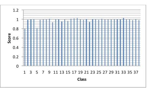
The confidence level is the second critical parameter introduced in this study, it measures the amount of conviction of the classifier as the distance between the score of the winner class with the one of the runner up. To better illustrate this concept, we run the pre-definite experiment on the Extended Yale B database (38 classes) and we saved in Figure 3.1 the set of residuals which allow for correct classification of a test sample and in Figure 3.2 the set of residuals which bring to misclassify the current test sample.
Figure 3.1 Residuals of a correct classified test sample
Figure 3.2 Residuals of a misclassified test sample
While in Figure 3.1 the score of class 1 is obviously the little one and there is no uncertainty in declaring class 1 as the winner class, in Figure 3.2 the decision of SRC is not as clear as before because the score of the winner and the one of the runner up
0 0.2 0.4 0.6 0.8 1 1.2 1 3 5 7 9 11 13 15 17 19 21 23 25 27 29 31 33 35 37 Sc or e Class 0 0.2 0.4 0.6 0.8 1 1.2 1 3 5 7 9 11 13 15 17 19 21 23 25 27 29 31 33 35 37 Sc or e Class
![Figure 2.3 Sparse versus compressible signals (courtesy of Boufounos et al. [22]) During the sampling step, to ensure a lossless mapping, it is necessary to impose strong assumptions on the structure of the dictionary D , which mu](https://thumb-eu.123doks.com/thumbv2/9libnet/3256086.8345/24.893.169.776.535.704/compressible-courtesy-boufounos-sampling-necessary-assumptions-structure-dictionary.webp)