Efficient methods for electromagnetic characterization of 2-D geometries in stratified media

■

ттЛ^^'^тжШ Щ Щ ■

.р р ію м Ж Ш Е З Ш;.: ■

EFFICIENT METHODS FOR ELECTROMAGNETIC

CHARACTERIZATION OF 2-D GEOMETRIES IN

STRATIFIED MEDIA

A TH ESIS

SU B M ITT ED TO TH E D EPA R T M E N T OF EL EC TR IC A L AND ELECTRO N ICS EN G IN E ER IN G

AND T H E IN S T IT U T E O F E N G IN E ER IN G AND SCIENCES

OF B ILK EN T U N IV ER SITY

IN PARTIAL FU L FIL LM EN T O F T H E REQ U IREM EN TS

1 FO R T H E D E G R E E OF M A STER O F SC IEN CE

By

Fatma Çalışkan

August 1997

I certify tlrat I have read this thesis and th a t in iny opinion it is fully adequate, in scope and in quality, as a thesis for the degree of M aster of Science.

(J j .

Assoc. Prof. Dr. M. Irşadi Aksun (Supervisor)

I certify th a t I have read this thesis and th a t in my opinion it is fullj^ cidequate, in scope and in quality, as a thesis for the degree of Mcister of Science.

Prof. Dr. Ayhcui A ltıntaş

I certify th a t I have read this thesis and th a t in iny opinion it is fully a.dc(|uate, in scope and in quality, as a thesis for the degree of M aster of Science.

soc:. Prof. Dr. (-liilbin Dm■a.,1

Approved for the In stitu te of Engineering and Sciences:

Prof. Dr. Mel^jiifit Baray

EFFICIENT METHODS FOR ELECTROxMAGNETIC

CHARACTERIZATION OF 2-D GEOMETRIES IN

STRATIFIED MEDIA

Fatma Çalışkan

M.S. in Electrical and Electronics Engineering

Supervisor: Assoc. Prof. Dr. M. İrşadi Aksun

August 1997

Numerically efficient method of moments (MoM) algorithms are developed for and applied to 2-D geometries in multilayer media. These are. namely, the spatial- domain MoM in conjunction with thi? closed-form Green's functions, the spectral- domain MoM using the generalized pencil of functions (GPOF) algorithm and a FFT algorithm to evaluate the MoM matrix entries. These approaches are mainly to improve the computational efficiency of the evaluation of the Mo.M matrix entries. Among these, the spectral-domain MoM using the GPOF algorithm is the most efficient approach for printed multilayer geometries. The assessment of the efficiency of this method is performed on several problems, by comparing the matrix fill times for these three approaches. In addition a new iterative algorithm

is developed to solve the MoM matrix equation, which is based on dividing a large object into subregions and solving the matrix equation on each subregion by considering the effects of other regions. This iterative algorithm is applied to some large geometries and is compared to a traditional LU decomposition algorithm for the assessment of its numerical elBciency. It is observed that the iterative algorithm is numerically more efficient as compared to the LU decomposition.

Keywords : Method of moments, Planarly layered media. Green's functions, It­

erative method

ÇOK KATMANLI ORTAMLARDA 2 BOYUTLU

GEOMETRİLERİN ELEKTROMANYETİK TANIMLAMASI

İÇİN ETKİLİ YÖNTEMLER

Fatma Çalışkan

Elektrik ve Elektronik Mühendisliği Bölümü Yüksek Lisans

Tez Yöneticisi: Doç. Dr. M. İrşadi Aksun

Ağustos 1997

Çok katmalı ortamlarda 2 boyutlu geometriler için sayısal olarak etkin moment metodu (MoM) algoritmaları geliştirildi ve 2 boyutlu geometrilere uygulandı. Mo.M matris elemanlarını hesaplamak için kullanılan yöntemler, kapalı formda Green fonksiyonları ile birlikte kullanılan gerçek uzay moment metodu, general­ ized pencil of functions (GPOF) algoritması kullanılarak yapılan spektral uzay moment metodu ve moment metodu matris elemanlarını hesaplamak için hızlı Fourier döııüşümii (FFT) algoritması kullanılmasıdır. Bu yöntemler moment metodu matris elemanlarını işlemsel olarak verimli bir şekilde bulmak için kul­ lanırlar. Bu yöntemler içinde çok tabakalı basılı geometriler için en etkili olan CROP' algoritması kullanılarak yapılan spektral uzay moment metodudur. Bu

metodun etkili olduğu bir çok problem üzerinde üç metodun matris eleman­ larını hesaplama süreleri karşılaştırılarak gösterildi. Buna ek olarak moment metodu matris denklemini çözmek için yeni yinelemeli bir algoritma geliştirildi. Bu 3'öntem büyük bir nesneyi alt bölgelere parçalayıp, her bölgenin matris den­ klemini diğer bölgelerin etkilerini düşünerek hesaplamaktadır. Bu algoritma bazı bü}-ük geometrilere uygulandı ve sayısal etkisini değerlendirmek için geleneksel bir yöntem olan LU ayrıştırma algoritması ile karşılaştırıldı. Sonuç olarak, yinelemeli algoritmanın LU decomposition algoritmasından saAusal olarak daha etkili olduğu gözlendi.

Anahtar Kelimeler : Moment metodu, Düzlemsel cok katmanlı ortam. Green fonksivonlari. Yinelemeli yöntem

I would like to express my deepest gratitude to Assoc. Prof. Dr. M. İrşadi .Aksun and Asst. Prof. Dr. Levent Gürel for their supervision and encouragement in all steps of the development of this work.

I would like to thank Prof. Dr. Ayhan .Altıntaş and .Assoc. Prof. Dr. Giilbin Dural for reading and commenting on the thesis and for the honor they gave me by presiding the jury. I would also like to thank Prof. Dr. Erdem \ azgan and .Asst. Prof. Dr. .Adnan Koksal for supporting me during my undergraduate studies.

.Many thanks to Noyan. Ertem, Tolga, Çiğdem. Deniz. Kürşal. Karim. .Ay­ han and Tunç for their valuable help. Sincere thanks are also extended to my officemates Erdem, Fehmi and .Moez. I also thank all my friends for their moral support.

It is a pleasure to express my special thanks to my family, especially to my mother, father and Zeynep, for their endless love, patience, support and encour­ agement .

To my mother, father and Zeynep

1 Introduction 1

2 G reen’s Functions in Spectral and Spatial Dom ains 4

2.1 Green's Functions in the Spectral Domain 6

2.2 Closed-Form Green’s Functions in the Spatial Dom ain... 11

3 Formulation of Electric Field Integral Equation in 2-D 21 3.1 Method of Moments ... 22

3.2 Electric Field in 2 - D ... 24

3.3 Basis and Testing F u n ctio n s... 27

3.4 MoM Formulation in Spatial D o m a in ... 30

3.4.1 Singularity E x tra c tio n ... 32

3.5 MoM Formulation using F F T ... 34

3.6 MoM Formulation in Spectral Domain 39 4 Num erical Exam ples 42 4.1 Examples for the MoM Formulation in the Spatial Domain . . . . 43

4.1.1 .A Single Horizontal Strip ... 43 4.1.2 .Analytical Solution of Cylinders in a Homogeneous .Medium 48

4.1.3 A Conducting Cylinder in an Inhomogeneous Medium . . . 53 4.1.4 A Rectangular Cylinder in an Inhomogeneous Medium . . 55 4.2 Comparison of the M e th o d s ... 57 4.3 Examples for the MoM Formulation in the Spectral Domain . . . 64

5 Solving Linear Equations by the Iterative M ethod 73

5.1 Comparison of the Iterative Method and LU Decomposition 76 5.1.1 Example 1 ... 76 5.1.2 Example 2 ... 87 5.1.3 Example 3 ... 92

2 . 1 2.2 2.3 2.4 2.5 2.6 2.7 2.S 3.1 3.2 3.3 3.4 4.1

Sources embedded in a multilayer medium... 7 Definition of the Sommerfeld integration path, and the paths C’opi and Cop2 used in two-level approximations... 14 The magnitude of the Green’s function for the vector potential 18 The magnitude of the Green’s function for the vector potential G 'l 18 The magnitude of f G ^ ^ d x ... 19 The magnitude of the Green’s function for the vector potential 19 The magnitude of the Green's function for the scalar potential Gj' 20 The magnitude of the Green's function for the scalar potential G?' 20 Strip of width 2«’ located near interface between two semi-infinite half-spaces and illuminated by source in upper half-space... 26

0 and Q on basis and testing fu n c tio n s ... 28 Single triangular testing and basis f u n c tio n s ... 29 Basis and testing functions on a single horizontal strip of width 2w 33 Strip of width 2ir located near interface between two semi-infinite half-spaces and illuminated by source in upper half-space... 43

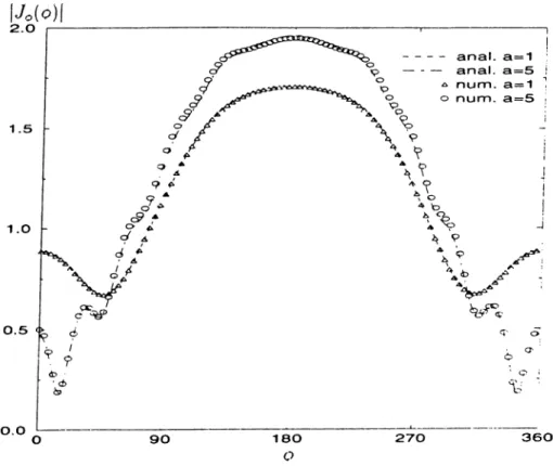
4.2 Normalized current density on a four wavelength strip for the TM excitation (reproduced from [15]). See Fig. 4.1 and the following text for the geometry and its parameters... 4-5 4..3 Normalized current density on a four-wavelength strip from the

spatial-domain ^íoM for the TM excitation. See Fig. 4.1 and the following text for the geometry and its parameters... 4-5 4.4 Normalized current density on a strip below interface for ^ = 0°

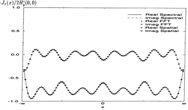
and the TM excitation (reproduced from [16]). See Fig. 4.1 and the following text for the geometry and its parameters... 46 4.5 Normalized current density on a strip below interface for 6 = 0°

and the TM excitation from the application of the spatial-domain MoM. See Fig. 4.1 and the following text for the geometry and its parameters... 46 4.6 Normalized current density on a strip below interface for 6 = 0°

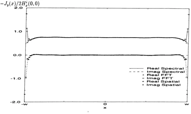
and the TE excitation (reproduced from [17]). See Fig. 4.1 and the following text for the geometry and its parameters... 47 4.7 Normalized current density on a strip below interface for 6 = 0°

and the TE excitation from the application of the spatial-domain MoM. See Fig. 4.1 and the following text for the geometry and its parameters... 47 4.S .A plane wave incident upon a conducting cylinder in a homoge­

neous m edium ... IS 4.9 The magnitude of the current density on a cylinder in a homoge­

neous medium for TM excitation 52

4.11 Conducting cylinder located near interface between two semi-infinite half-spaces and illuminated by a plane wave in upper half-space. . 53 4.12 Normalized current density on a circular cylinder of radius R =

0.375Ao for the TM excitation with various sampling points along the circumferential direction. See Fig. 4.11 and the following text for the geometry and its parameters... 54 4.13 Rectangular cylinder located near interface between two semi-infinite

half-spaces and illuminated by a plane wave in upper half-space . 55 4.14 Normalized current density on a rectangular cylinder of cross sec­

tion 0.25Aa (width) and O.lAg (height) for the TM excitation with various sampling points along the periphery. .See Fig. 4.13 and the following text for the geometry and its parameters.

4.15 .Normalized current density on a rectangular cylinder of cross sec­

tion 0.25Aa (width) and O.lAa (height) for the TE excitation with various sampling points along the periphery. See Fig. 4.13 and the following text for the geometry and its parameters.

4.16 The real and imaginary parts of the normalized current densities for the TE excitation and for 0 = 0·^

4.17 The real and imaginary parts of the normalized current densities for the TE excitation and for 6 = - 4 5 '^ ... 58 4.18 The real and imaginary parts of the normalized current densities

56

56

58

for the T.M excitation and for 6 — O'’ 59

4.19 The real and imaginary parts of the normalized current densities for the TM excitation and for 0 = —45° 59 4.20 Normalized current densities on the strip for the TE excitation and

h = -0.1 Afc 61

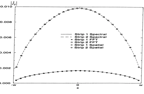
4.21 Normalized current densities on the strip for the TM excitation and h = —O .lA j,... 61 4.22 A two-strip, three layer geometry... 62 4.23 The magnitudes of the current densities on the two strips for the

TM excitation 63

4.24 The magnitudes of the current densities on the two strips for the TM e.xcitation... 63 4.25 A geometry of ten strips located side by side in a homogeneous

medium... 65 4.26 The magnitude and phase of the current densities for the TE ex­

citation, and for kw = 1 . 0 ... 66 4.27 The magnitude and phase of the current densities for the TE ex­

citation. and for kw = 2 . 0 ... 66 4.28 The magnitude and phase of the current densities for the TE ex­

citation. and for kw = 3 . 0 ... 67 4.29 The magnitude and phase of the current densities for the TE ex­

citation, and for kw = 4 . 0 ... 07 4.30 The magnitude and phase of the current densities for the TE ex­

citation. and for kw = 5 . 0 ... 08 4.31 The magnitude and phase of the current densities for the T.M ex­

citation, and for kw = 1 . 0 ... 08

4.33 The magnitude and phase of the current densities for the TM ex­ citation, and for kw = 3 . 0 ... 69 4.34 The magnitude and phcise of the current densities for the TM ex­

citation, and for kw = 4 . 0 ... 70 4.35 The magnitude and phase of the current densities for the TM ex­

citation, and for kw = 5 . 0 ... 70 4.36 Three strips located in the same m ed iu m ... 71 4.37 The magnitudes of the current densities on the three strips for the

TE e x cita tio n ... 72 4.3S The magnitudes of the current densities on the three strips for the

TM excitation... 72 5.1 Strip of width 2w located near interface between two semi-infinite

half-spaces and illuminated by source in upper half-space... 77 5.2 The current magnitude of the iterative method for the TM excita­

tion when iteration number is increasing for .V = 1000 84 5.3 The current magnitude of the iterative method and LI' decompo­

sition for the TM excitation and for N = 1000. 84 5.4 The current magnitude of the iterative method for the TE excita­

tion when iteration number is increasing for N = 1000 85 5.5 The current magnitude of the iterative method and LI’ decompo­

sition for the TE excitation and for N = 1000 ... 85 5.6 The error plot of the iterative method for the T.M excitation and

for ,V = 1000 ...

5.7 The error plot of the iterative method for the TE excitation and for N = 1000 ... 86 5.8 Two strips are located parallel to each other where the distance

between them is A2... 87 5.9 The magnitude of the current densities for the iterative method

and LU decomposition for the TM excitation, A’=1000 and exam­ ple 2 ... 91 5.10 The magnitude of the current densities for the iterative method

and LU decomposition for the TE excitation, A’=1000 and exam­ ple 2 ... 91 5.11 Three strips of width 2w located in homogeneous medium with

0.5u> spacing between them on the same r ... 92 5.12 The current magnitude of the iterative method and LU decompo­

sition for 0 = 0° and TM e x c ita tio n ... 9-1 5.13 The current magnitude of the iterative method and LU decompo­

sition for 0 = and TM e x c ita tio n ... 94 5.14 The current magnitude of the iterative method and LU decompo­

sition for ^ and TE e x c ita tio n ... 95 5.15 The current magnitude of the iterative method and LU decompo­

sition for 0 = 60‘^ and TE excitation 95

4.1 4.2 4.3 5.1 5.2 5.3 5.4 5.5 5.6

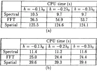
The CPU times of the spectral domain, the spatial domain and the FFT approaches for TE and TM excitations 60 The CPU times of the spectral domain, the spatial domain and the FFT approaches for (a) TE and (b) TM excitations 62 The CPU times of the spectral domain, the spatial domain and the FFT approaches for the TE and TM excitations... 64 The values of A’l and N2 for different N for example 1... 7S (a) The CPU times of the iterative method and LU decomposition (b) The number of iterations of the iterative method for the TM excitation and example 1.

The CPU time and number of iterations of the iterative method for the T.M excitation when N is set to (a) 200. (b) 400.

(a) The CPU times of the iterative method and LI decomposition (b) The number of iterations of the iterative method for the TE

excitation and example 1. S2

The CPU time and number of iterations of the iterative method for the TE excitation when .V is set to (a) 200. (b) 400... S3 The values of A'l and .V> for various A’ for example 2... SS SO

SI

•5.7 (a) The CPU times of the iterative method and LU decomposi­ tion (b) The iteration number of the iterative method for the TM

excitation and example 2. 89

5.8 (a) The CPU times of the iterative method and LU decomposi­ tion (b) The iteration number of the iterative method for the TE

excitation and example 2. 90

5.9 The CPU times of the iterative method and LU decomposition for (a) TM and (b) TE excitations and (c) the iteration numbers of the TM and TE excitations when 0 is 0° and 60'^... 93

In trod u ction

Advances in high speed digital computers have led to the development of more sophisticated numerical methods to solve large electromagnetic problems of prac­ tical interest which, by classical techniques, would be virtually impossible. The basic techniques that are used in electromagnetic problems are mainly the method of moments (MoM) [1. 2]. finite element methods (FE.M) [3] and the finite differ­ ence time domain (FDTD) methods [4], all of which basicly transform integral, differential or integro-differential equations into algebraic equations. Therefore, the computational efficiency of these techniques is dependent on the efficiency of forming a set of linear equations and the number of unknowns.

The Method of Moments is very popular for the solution of open field prob­ lems.. particularly for printed geometries in planar stratified media. It is presently recognized as the most powerful approach for the analysis of printed antenna con­ figurations and for the characterization of radiation and coupling phenomena in printed circuit discontinuities. .A large number of applications of the .\loM can be found in the literature [5. 6. 7].

Chapter 1. Introduction

The main advantages of MoM are its accuracy, versatility and the ability to compute near -as well as far-zone parameters. The basic idea of the MoM is to reduce an integral equation to a matrix equation, and to solve the matrix equation by a known technique.

The first step of the MoM formulation is to write an integral equation describ­ ing the electromagnetic problem, which could be the mixed potential integral equation (MPIE) or the electric field integral equation (EFIE) for the printed geometries. These integral equations require related Green's functions, either of the vector and scalar potentials (for MPIE formulation) or of the electric fields (for EFIE formulation). Since the spectral-domain Green's functions are available in closed forms, their spatial-dotnain counterparts are obtained via an efficient inverse Fourier transform algorithm. Once the Green's functions are obtained, the solution due to a general source in 2-D can be obtained by the principle of linear superposition. The next step in the MoM formulation is to expand the unknown function in terms of known basis functions with unknown coefficients, then is to implement the boundary condition in integral sense through the testing procedure. Following these steps, the integral equation is transformed to a matrix equation, whose entries are double integrals in the spatial domain, one for the convolution integral to find the electric field, and one for the testing procedure to apply the boundary condition. However, in the spectral-domain application of the .Mo.M. the matrix entries become single integrals over infinite domain. Con­ sequently. the computational efficiency of the MoM lies in the evaluation of the MoM matrix entries, of course for moderate size geometries requiring a few hun­ dred of unknowns. For a geometry requiring a large number of unknowns, the

matrix solution time dominates the overall performance of the technique, there­ fore the efficiency of the method is defined by the efficiency of the linear s} stem solver.

In this thesis, three different implementations of the MoM are studied, which are, namely, the spatial-domain MoM using the closed-form Green's functions, the spectral-domain MoM using the GPOF algorithm [10] to find the matrix entries, and the spectral-domain MoM using a FFT algorithm to evaluate the matrix entries. It is observed that the most efficient one is the spectral-domain MoM using the GPOF algorithm. However, for large geometries requiring a large number of unknowns, the efficiency of the overall method can be improved by using an iterative algorithm, developed in this thesis, for the solution of the matri.x equation.

In Chapter 2, a method to obtain Green's functions in the spectral and spatial domains is presented. The details of the MoM formulations in the spectral and spatial domains are given in Chapter 3. Then, several numerical examples of these approaches are presented in Chapter 4. .An efficient iterative method to solve the matrix equation is introduced in Chapter 5 with some examples, and finally, conclusions and future work are given in Chapter 6.

C hapter 2

G reen ’s F unctions in S p ectral

and Spatial D om ain s

Green's functions, either in the spatial or spectral domain, play an important role in driving integral equations for electromagnetic problems. Especially for planar multilayer geometries, they reduce the dimension of the problem from .3-D to 2..5D by incorporating the layer information, such as the dielectric constants, thicknesses and the number of layers, through satisfying the boundary conditions at the interfaces between the layers. Therefore, the efficient calculation of Green's functions is quite important for the efficiency of the method employed in the characterization of such geometries. In this chapter, the derivation of Green's functions in the spectral domain is first presented, then their spatial domain counterparts are obtained in closed forms.

Green’s functions of the vector and scalar potentials in the spectral and spa­ tial domains are obtained for the sources of horizontal and vertical elect ric dipoles

placed in multilayer planar media, where the layers are assumed to extend to in­ finity in transverse directions. The spatial-domain Green’s functions are obtained by taking the inverse Fourier transform of the corresponding Green's functions in the spectral domain whose analytical expressions are available for planar, mul­ tilayer geometries. Hence, the main difficulty in obtaining the spatial-domain Green’s functions is the transformation of the spectral-domain Green’s functions, which can be done analytically for a few special cases. Here, we present a tech­ nique that will allow the spatial-domain Green’s functions to be approximated in closed forms, and that will completely eliminate the computational difficulty.

To obtain the inverse Fourier transform analytically, Green’s functions in the spectral domain are approximated in terms of complex exponentials. One way to perform this approximation is to use Prony’s method, in which the number of samples required must be twice the number of complex exponentials [8]. It is obvi­ ous that this leads to difficulty in sampling rapid variations of the spectral-domain Green's functions, unless a large number of exponentials is used. .Although the least-square Prony method improves its ability to account for the rapid changes with a moderate number of exponentials [9], it still requires several trial and error iterations, because of its noise sensitivity, which makes the technique inefficient and not robust. .Another exponential approximation technique is the generalized pencil of function (GPOF) method [10]. which is more robust and less noise sen­ sitive when compared to the original and least-square Prony methods, and also provides a good measure for choosing the number of exponentials required in the approximation. However, it still requires a study of the spectral-domain behav­ ior of the Green's function in advance, in order to decide on the approximation parameters such as the number of sampling points and the maximum value of

the sampling range. In addition, one would need to take thousands of samples in order to be able to approximate a slow converging function with rapid changes, because both the Prony and the GPOF methods require uniform sampling of the function.

Recently, a new approach based on a two-level approximation has been pro­ posed to overcome the previously mentioned difficulties, and it has been demon­ strated that the new approach is very robust and computationally much more efficient than the original one and its variants. The two-level approach divides the range of approximation into two parts, the first one covers the region where the function to be approximated has rapid transitions, whereas the function is smooth in the second region. Therefore, it is no longer necessary to take thou­ sands of samples to account for a rapid transition that occurs in a small part of the entire range, resulting in a significant reduction in the number of data points to be processed, which, in turn, translates into a substantial saving in the computation time.

We will derive the spectral-domain Green's functions for planarly stratified media in Section (2.1). and will present the method of obtaining the closed-form spatial domain Green's functions in Section (2.2).

2.1

G reen’s Functions in th e Spectral D om ain

Chapter 2. Green’s Functions in Spectral and Spatial Domains 6

Consider the planar multilayered medium shown in Fig. 2.1 where it is assumed that the layers extend to infinity in the transverse directions. The source, (hor­ izontal electric dipole (HED) or vertical electric dipole (VED)) is embedded in region / and the observation point can be located in an arbitrary layer. Each

layer can have different electric and magnetic properties (tr,,//r, ) and thickness (</,). Perfect electric conducting planes and half-spaces are also regarded as layers in this formulation.

A ^

region -(i-i-m )

region -(i+ 1 )

re gio n -(i) so urce

(H E D ,V E D ,H M D ,V M D ) re g io n -(i-l) re g io n -(i-m ) z=z m-h 2=d j-h - z= -h - z= -d -h -m-h

Figure 2.1: Sources embedded in a multilayer medium.

The spectral-domain Green's functions are first derived in the source layer, then by using an iterative algorithm applied to each transverse electric (TE) and transverse magnetic (T.M) components they are obtained in the observation layer. Then, the spectral-domain Green's functions are approximated in terms of complex exponentials via the GPOF method after the direct terms have been extracted.

All of the Green's functions, presented herein, are for the vector and scalar potentials that are indeed not defined uniquely in stratified media [11]. In other words, different sets of Green's functions for the vector and scalar potentials can be chosen to satisfy the same boundary conditions. The following notation for

Chapter 2. G reen’s Functions in Spectral and Spatial Domains

the Green’s function is commonly used and referred to as the traditional form:

Ga (t x “{■ yy')GXX “f“ ^xGXX “f" zyGxy "h -^zGXX (2.1)

for the vector potentials, 6’’' and G’* for the scalar potentials.

The spectral-domain Green’s functions of the vector and scalar potentials can be obtained from the electric and magnetic fields generated by a current dipole J = /oM(r)o, where o is a unit vector. For the sake of illustration, the field components for an HED in a multilayer media. Fig. 2.1, can be written in the source layer (layer i) in 2-D as follows [12]:

h i / oo

■00 (2.2)

4/· J-oc Kz,

k

(2.3) where the z dependence of the fields in the source region is characterized as the sum of the direct term and up- and down-going waves due to the reflections from the boundaries at z = —h and c = d, — h. respectively, where -f and — signs are for positive and negative c values, respectively. The coefficients of the up- and down-going waves can be obtained in terms of the generalized reflection coefficients by applying the appropriate boundary conditions: (i) the down-going waves for r > 0 are the consequence of the reflections of the up-going waves at c = d, — h: (ii) the up-going waves for c < 0 are the consequence of the reflections of the down-going waves at c = —h. It should be noted that the other field components can be easily derived from the z-coniponents of the fields [12]. so they are not included here. After having obtained the field components, the components of the vector potential and the scalar potential can be derived from

the following relations: Od = -■ V X A = //,H V X A loi do (2.4) (2.5) ju^piCi ju) dV

where Pd and p are the scalar potentials for the dipole element and a point charge, respectively, and I' is replaced by x' for an HED and replaced by for a VED. Below are the expressions of the spectral-domain Green's functions (traditional form) in the source layer for HED and VED sources. They read:

HED: Gi, = ~ {£-'‘'■.1'' + /IJe'*··-- + a e -''·-··} (2.6) G i = ÿ f r (2.7) 6·;· = - i — 1(2. 8) [ >'r f'i ) \E D : 22A-,,e. i J (2.9) (2.10)

where Gfj denotes the spectral-domain Green's Tmctions for the vector potential in the direction-? due to a unit _/-directed current element, G^' represents the Green's function of the scalar potential in the spectral domain due to a unit /-directed electric current element, = kj -f the superscript .1 represents

C hapter 2. Green’s Functions in Spectral and Spatial Domains 10

the electric vector potential, and qg represents the electric scalar potential. The coefficients, „ and are functions of the generalized reflection coefficients Rte.t m, and they are given by

(2.11) = (2.12) Cl (2.13) Dl = (2.14) K (2.15) B l = (2.16) Q (2.17) D[ = (2.1S) where Ai, = [I - \ pj + l j I bhJ-1 ..-J*··--, 2rf; r> J + l.J ^ T E . T M + ^ T E . T M ^ ^ T E . T . M - , p p j . J - 1 Wj 1 — ^j.J + i^TE.TM^ (2.19) (2.2 0)

Here R and R are the Fresnel and the generalized reflection coeiiicients [12] for which the subscripts T E and T .l/ represent the polarization of tiu' wa\'e. the

superscripts (î, ; — 1) or (i.i + 1) show the layer numbers, the subscripts h and used in the coefficients (2.11)-(2.18) represent the orientation of the source, horizontal and vertical, respectively, while the superscripts e denotes the electric current source.

The amplitudes of the up- and down-going waves in a layer different from the source layer are related to those in the adjacent layers by.

A- _ J - + ___________________ _(2.21)

where A~ and are the amplitudes of the down-going waves in layers j and

j + 1. respectively, {j = i — m), T is the transmission coefficient, and Z-m is

the distance between the lower boundary of the source layer i and the lower boundary of layer j . Fig. 2.1. Sirtiilarly the amplitudes of the up-going waves in layer j = i + m can be written as

T i )(-m-i +d,-h)

4-1- ^ A+ ______

‘ j ■ 1 _ D. D , (2.22)

Therefore, starting from the source layer, the field e.xpressions for any layer can be obtained iteratively.

2.2

C losed-Form G reen’s Functions in th e Spa­

tial D om ain

The scalar wave equation of a line source is written as

0(.r.c) = -<^(.r)6(r) +

Chapter 2. Green's Functions in Spectral and Spatial Domains 12

Because of the cylindrical symmetry of the problem, Eq. (2.23) is solved in cylin­ drical coordinates, i.e.,

1 d

+ - ^ + ki M = - Hp) dp^ pdp

where 6{p) = ¿(x)S(z). It is known that, the solution of Eq. (2.24) is given as (2.24)

o M = (2.25)

In addition, Eq. (2.23) can be solved by Fourier transform technique. For a fixed z, assuming that the Fourier transform of (p{x,z) exists, then it is expressible as an inverse Fourier transform integral as

= ^ r z)e-^^^-dkr (2.26)

¿7T J-oo

Consequently, on substituting (2.26) into (2.23), and using the fact that

<^(-r) = ^ r w 7T */ — CO (2.27) one obtains 1 r 2k L · . I 5,-2 ¿(A v ,-')e --''-^"d A v = 2x J-c<

r H = K^'^''(lkr

Therefore, we must have

+ à { k , . z ) = : - S ( = ) (2.29)

where kj = k'l - kj. Thus.

o(kr.=) = -^—

2k. (2..30)

if only the outgoing-wave solution is considered. Hence. Eq. (2.26) becomes

By the uniqueness of the solution to the partial differential equation (2.23). Eq. (2.31) must be equal to Eq. (2.25) since both of them satisfy (2.23). As a result, an integral identity

I r<x

i /

n J -C -dkr (2.32)

is obtained, which is used throughout this thesis quite frequently. The right- hand side of Eq. (2.32) could be interpreted as an integral summation of the plane waves propagating in different directions including evanescent waves [12].

Since the principal goal of this section is to introduce a robust and efficient technique to obtain the spatial-domain Green’s functions in closed-forms for pla­ nar layered media, it would be useful to first provide the definition of the spatial- domain Green’s functions

1 qA.i. = — r

'¿■K J-<x. (2.33)

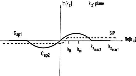
where, G and G are the Green's functions in the spatial and spectral domains, respectively, and S I P is the Sommerfeld integration path defined in F'ig. 2.2.

The integral given in (2.33) cannot be integrated analytically, except for a few special cases. However, if the spectral-domain representation of the Green's function. G in the integrand can be approximated in terms of complex exponen­ tials. the analytical evaluation of the integral (2.33) becomes possible and can be expressed in terms of summation of the Hankel functions of the second kind. Therefore, the crucial step in the derivation of the closed-form Green's functions is the exponential approximation of G.

The original approach of getting the closed-form Green's functions in the spatial domain has had some difficulties for example, the quasi-dynamic images and the surface wave poles need to be found and extracted from the Green's

Chapter 2. Green’s Functions in Spectral and Spatial Domains 14

Re[kv]

Figure 2.2: Definition of the Sonunerfeld integration path, and the paths Cap\ and Cap2 used in two-level approximations.

function prior to the approximation. However, with the introduction of the two- level approach, which is robust and very efficient, these difficulties are eliminated [1.3]. In the two-level approach, a path formed by the paths Cap2 and Capi is employed, as depicted in Fig. (2.2). and the paths Cap\ and Cap2 ai«* defined by the following parametric equations:

For Capi k,, = + /] 0 < / < Jcl (2..34) /

For Cap2 K = A-.[-it + ( l - — )] 0 < / < ro, 12.35) Jo2

where i is the running variable sampled uniformly in the corresponding range. The exponential approximation process begins with sampling the function to be approximated, and then the algorithm for exponential approximation is employed for the sampled values of the function. .After having sampled the spectral-domain Green's function to be approximated, apart from the term l//2 ^ :,. the GPOF' method is used to obtain the exponential approximation of the function, which

results in an approximation as follows: G = J i K \ n i = l A3 H2=l T13=1 Ni ) + E \ (2.36)

ri2 = l

J

where C„’s and a „ ’s denote the coefficients and exponents of the complex expo­ nentials obtained via the GPOF method.

To demonstrate the procedure on a real example, the derivation of the closed- form Green’s function in the spatial domain G^^ is given below: first, the spectral domain representation is written

;2L , i t I

+ (2.37)

then its approximation by complex exponentials is transformed into the spatial domain as (2.38) 1 2 ; r i : d k j . 6 - j k z T ^ A _{T I} El r d k ^ e -2 IT J - x ■V2XX £ ~ ^ ^ 2xx ^*‘ 1 +

E

E

Chapter 2. Green's Functions in Spectral and Spatial Domains 16

derived in Eq. (2.32), the spatial-domain Green’s function is obtained as

G t =T X ' 4 _{^ ^ I x x — 1 n 2 x x - - l} + L p „ „ ) + I (2-10) H 3 x x = l n 2 x x = l ) where P = \J{i - I ' Y F {z - z'Y (2.41) Pn,ss = + + z'+jo„,^^Y (2.42) pn\L = \/(^ “ + (2 - + io n ,„ Y (2.43) Æ = \/(^ ~ + { z - z ' - Y (2.44) Pnzzz = v/(^ - ^ ' Y + (^ + u - ;o„3„ Y (2.45) It is known that Gy^ is equal to and the formulation procedure for G'J'. GV and Gf, are similar to G'^^.. For the derivation of one should note that Av in the numerator of its spectral domain representation (2.7) should be eliminated in the approximation process. Therefore, —jkj. is taken out from the expression, and G-^^l{-jkj·) is approximated:

^

- j k r 2jF, [ j k i ikï (2.16)

n2rx = l

Tî3;j = l ^2rx — Î Using the following property of the Fourier transform.

G (.r.r) <— > G(k^.:) 6'(Av.-‘ )

J d.rG(x. :)

the integral of 6’^^. is obtained as J d r G i = Y pi\>J . V , „ .V3xx

E

Since the derivative of Hankel function is given by

dx = - a H ^ ^ \ a x ) (2.51)

Gil can be obtained as

G i = - 4- ( E c . J ~ n ? { h p. „. ) + Y

[nux = l Pri\zz , _{rî2rx = l}

_Æl

N--x3

+ G nj . ,

n3rx = l P^2zx ri2zx = l rî2*i = l P'r\2zx ^

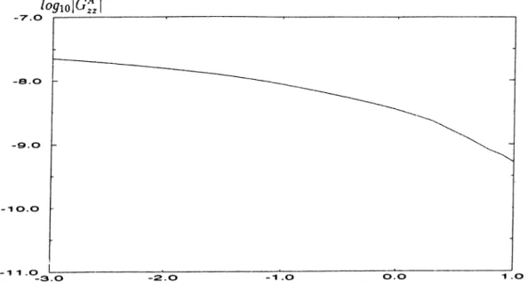
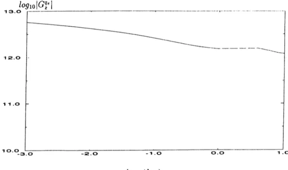
To give an idea how these closed-form Green’s functions behave, an example is provided for two layer media: the first layer has a relative permittivity of 4 and the second layer is free space, the source is placed at the interface and hence c = c' = 0 . The plot of Green’s functions are given below.

Chapter 2. Green’s Functions in Spectral and Spatial Domains 18

¡ogio(koP)

Figure 2.3: The magnitude of the Green’s function for the vector potential

logio\Gi

logio{fcop)

logiol I Gf.dx\

, logio{kop)

Figure 2.5: The magnitude of / G^^dx

logio\Gi^

logxo{kop)

Chapter 2. G reen’s Functions in Spectral and Spatial Domains 20

logioiKp)

Figure 2.7; The magnitude of the Green’s function for the scalar potential GJ'

logw{f''op)

Form ulation o f E lectric Field

In tegral E quation in 2-D

Method of Moments is one of the most popular numerical techniques employed in electromagnetic simulations of printed circuits, and antennas. Hence, in this thesis we are mainly concerned with the analysis of 2-D printed structures with the use of the various forms of the MoM. Although the main algorithm is the same in these forms, which is the discretization of unknown in terms of known basis functions and application of the boundary condition: in integral sense, the implementation of these steps can be carried out in different domains or via different algorithm. For e.xample, the whole algorithm can be carried out in the spatial and spectral domain, or the implementation of the boundary condition in integral sense can be performed via the fast Fourier transform.

Chapter 3. Formulation o f Electric Field Integral Equation in 2-D 00

3.1

M eth o d o f M om ents

Although the MoM in this thesis is applied for the solution of an integral equation, the general setting of the MoM is given here for the sake of completeness. For this purpose, the following operator equation is considered,

LU) = g (3.1)

where g represents a known source contribution, L denotes a linear operator operating on an unknown parameter / , that has to be determined. The first step in the application of the MoM for the solution of Eq. (3.1) is to expand the unknown parameter by a set of known basis functions with unknown coefficients as

/ = I ] o n /n (3.2)

n

where fr, represents the basis function spanning the domain of the operator L. and On is the corresponding unknown coefficient. Using the representation of / in Eq. (3.2) and the linearity property of Z, the following equation is obtained :

Y^o„L{f„) = g (3.3)

The second step in .Mo.M is to use a set of weighting functions, or testing functions, u’l. <C2. {<’3.... in the range space of Z. and to take their inner products with both sides of Eq. (3.3). resulting in

< > = X lf'n < U'l.I.fn >

Tl

These equations can be written in matrix form as [^m] — [fmn][ûn] where [^m] — < wi.g > < W2.g > [/.„) = < IÜ1,1 / , > < u>,,

_¿/2

If the matrix [/] is nonsingiilar, then

[ ^ n ] [^m n] [i7m]

(3.5)

(3.6)

(3.7) ami the solution for / is obtained from Eq. (3.2). If the matrix [/] is of infinite order, then its inversion can not be performed unless [/] is tliagonal. If the sets /„ and tVn are finite, the matrix is of finite order, and can be inverted by known methods.

The solution depends on the choice of the basis functions, whicli should be linearly independent and should be chosen such that some linear combination Eq. (3.2) can approximate / reasonably well. The solution also d('])ends on the set of testing function u'j.ti'i... which should be linearly indepi'iuhmt and should best represent the properties of g. Some additional factors which alfect

Chapter 3. Formulation o f Electric Field Integral Equation in 2-D 21

the choice of /„ and U’„ are (1) the accuracy of solution desired. (2) the ease of evaluation of the matrix elements, (.3) the size of the matrix that can be inverted, and (4) the realization of a well-conditioned matrix [/] [1].

The name method of moments derives from the original terminology that

j is the nth moment of / . When x ” is replaced by an arbitrary »·„. we continue to call the integral a moment of / . The name method of weighted residuals derives from the following interpretation. If Eq. (3.3) represents an approximate equality, then the difference between the exact and approximate L f is

g - ' ^ O i n L f n = r (3.8)

n

which is called the residual r. The inner products < u \ . r > are called the weighted residuals. Eq. (3.4) is obtained simply by setting all weighted residuals to zero.

3.2

E lectric Field in 2-D

The general form of scattered electric fields can be written as

E, = - j i c G l * ^ · J)

Ey = (6’’^ * V · J) (3.10)

ny ‘ j w ay

E, = - j w G ^ * J , - j U-Gf^ * J y - j w G i * + "I;: · J ) (·^·' 0 where * denotes convolution, and G'^^ = G'^y The fields TV. Ey and IG n'presetit the scattered electric fields in .r. y and r directions, respectively. PIk' term 6',]

represents /-directed vector potential at r due to a ^-directed electric dipoI(' of unit strength located at r'. while (7’' represents the scalar pottnilial by a unit

point charge associated with an electric dipole. Since the traditional form of the Green’s functions is employed in the formulation, Green's function of the scalar potential is not unique for horizontal and vertical electric dipoles as stated previously. Hence, the term involving the Green's function of the scalar potent ial. which is common in Eqs. (3.9)-(.3.11 ). can be explicitly written as

* ^ + Gy * ^ + GV * ^ (•3.12)

dx ^ du ' dz

where Gj' = G’’' and G\’ denote Green's functions of the scalar potential for a horizontal and vertical electric dipoles, respectively. However, the equations (3.9)-(3.11) can be simplified in 2-D, because Jj, Jy and J; are functions of .r and r only, that is.

— (G’'* V - J ) = 0

ày

dy = 0

which result in the following scattered electric field equations:

El = —juzG^ * Ji -V jijj ax d d (3.13) (3.14) (3.1.5) e: = - J - K * Jy (.3.16) 1 d 0<; . + 6!· . (.3.17) Et = * Jr + G ·;, *J=) + — ^ ^ J a J C jZ

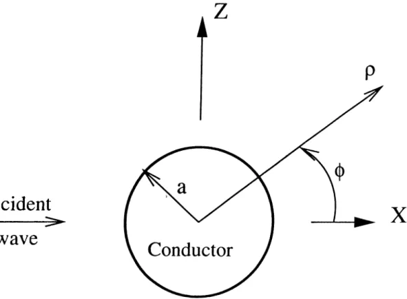
For the calculation of the incident field, a simple case in 2-D represented in Fig. 3.1 is considered. If the excitation is transverse electric (1 E) to //. then the magnetic field is in ^-direction, and written as

Chapter 3. Formulation o f Electric Field Integral Equation in 2-D 26

0

Figure 3.1: Strip of width 2w located near interface between two semi-infinite half-spaces and illuminated by source in upper half-space

Since the electric field integral equation is used throughout this thesis, the inci­ dent electric field is obtained from

V X H ' = _tf (3.19)

as

F· = + i-rF + f

tCf,

W hen the excitation is transverse magnetic (T.M) to >/. the electric field be­ comes in // direction, and written as

Since most of the examples in the literature are given as the current density normalized with respect to the incident magnetic field, this field component needs to be determined. From the following Maxwell’s equation

V X E ' =

1m (3.22)

the incident magnetic field is obtained as -1 U'/i,· V / where h _{= + «} (3.24) hr = sin 0 (3.25) = hi cos 0 (3.26)

and and are given in Eq. (2.20).

3.3

B asis and Testing Functions

The .Method of Moments converts an integral equation to a matrix equation and solves the matrix equation through the expansion of the unknown function in terms of known basis functions and weighting the resulting expression by the testing functions. Therefore, one needs to choose the basis and testing functions judiciously to minimize the error in average sense. Since the Galerkin method is used in the study, the basis and testing functions are chosen from the .same set of functions.

Chapter 3. Formulation o f Electric Field Integra! Equation in 2-D 28

thesis are presented. The current densities for TM and TE excitations are ex­ panded in terms of sub-domain basis functions as

M,r

Jy{v) — ^ ^ lym Fymiv)

m = l A/,c M v ) = ^ (3.27) (3.28) m = l

and the testing functions T„(u) are used as in Fig. 3.2, where u and v are functions of X and z.

Figure 3.2: o and o on basis and testing functions

These testing and basis functions are chosen as triangular functions. Fig. 3.3. and given by - <'i ( | ' 2 — <') ) ( f ' 3 - <'l ) 5 ( r ) = ^ <’3 - r .. if i·] < r < ('2 if 1'2 < i' < t’3 ((’3 — i’2)(C3 — i'l ) 0 otherwise (3.29)

where

and

Figure 3.3: Single triangular testing and basis functions

U — U |

if Í/1 < U < U2

T[u) = <

(U2 - Ui)(U3 - U])

---^---r if ll2 U < »3 ( » 3 - U 2 ) ( U 3 - Wl ) 0 otherwise o = ardan [ ^ ^ \-r3 --JÍ, .r = Vcos o = rs in o o = arctan ( i i z j . ) \X3 - Xi / .r = u cos o c = ?/sino

Chapter 3. Formulation o f Electric Field Integral Equation in 2-D 30

Since both the basis and testing functions are in the same form, the Fourier transform of the testing function is given here as

- ( U 3 - + ( « 3 - ( « 2

-T{h.) =

- U l ) ( « 3 - U l ) ( U 3 - U 2 )

(3.37) to be used in the spatial domain applications of MoM.

3.4

M oM Form ulation in Spatial D om ain

The total electric field for TE excitation in region i is the summation of the scattered electric fields and the incident electric field

E l = + zEt + E l

Similarly, the total electric field for TM excitation is written as

E'„, = HE- + E\_tm

(3.3S)

(3.39) Boundary conditions for the tangential electric fields for both TM and TE excitations are applied on the conducting body as

(-EL )fan = 0 and {El),an = 0 (3.10) and substituting Eqs. (3.3S) and (3.39) results in the following electric field inte­ gral equations (EFIE):

(.r£’; + i £f ) , . „ = -{El),„„ (3.41)

(.(/£*),„„ = (3.42)

With the application of the testing procedure of the Mo.M to these integral equa­ tions

for TE excitation, and

, El) = - {T,r.{v) . E\^) (3.44) for T.M excitation are obtained. Using the testing function of

Tvn(w) = Û T„„(u)

= (xcoso + f sino) rfn(l/) for TE case, the left hand side of Eq. (3.43) becomes

(Tvn(u) , vEl) = (T vn(«), xEl + zEt)

= J du (cosa £ ’* + sino' Et) T’,.„(i/)

= - j w /t-m [ / dl l r , . n ( u ) (cos Q COS 0 ( ?·)) m = l

+ y dw T v n i « ) ( s i n o CO SO G ';j. * 5 , . , „ ( r ) )

+ J du T„„{ti) ( sin O sin o Gf. * ¿?, m(<’))j I ( f j dl\,„(u) f -2 dB,.,r,(r) — — jy du — ;---- I cos O Gv * + j i « d u dT,.n(u) ( . 2 --- I Qir^ dl l sin^ 0 GV * dv dB,.,Jv)\ dr

and. the right hand side becomes

k-,H,

(Tvn(») . £") = [ / + 0)T,„{u)c·

— J dll cos(o -

d)f?^'0'r,.„(i/)f·'*^^'^“^-·''

(3.47)

== -M l

+ ^)7’,„(Â-sin(o +

ire,

- B'iiif,' cos(a -

0)f,,.(^-sin(d - o))r'<^'^"^-^--'‘"i'J(3.4S)

.Similarly, using the testing function of

Chapter 3. Formulation o f Electric Field Integral Equation in 2-D 32

for TM case, the left hand side of Eq. (3.44) becomes

(Tyn(ti) , y E 0 = - j w lym i du Ty„{u) G y y * By,„{v) (3.50)

m = l ■'

and the right hand side becomes (Tyo(«) , E') = J du

= £. [fy„(ks\n(Q + +R^'Ë^fyn{ksm{e

-(3.51)

(.3.52) .Since Green’s functions in the spatial domain are approximated as the sum­ mation of the Hankel functions of second kind, for small arguments they grow indefinitely and the integrals cannot be calculated efficiently. In order to solve this problem, a singularity extraction method must be used for small arguments.

3.4.1

Singularity E xtraction

The zeroth order Hankel function of the second kind H^^\k,p) has a logarithmic singularity for the argument kip 0.

H ^ ^ \ k , p ) ^ ' ^ H k , p ) (3..53) Therefore, in the calculation of Eqs. (3.16) and (3..50) for |n — < 1. the singularity extraction needs to be performed in order to find the self term [n = m) and the interaction between neighboring basis and testing functions.

To demonstrate the singularity extraction method on a simple example, a hor­ izontal strip in a homogent'ous medium is considered. Fig. 3.1. For 1 M excitation. Green's function is

K ^ A A A A ^ |N / \ / \ / \ / \ / | | N ^ \ / \ / \ / \ / \ / | ^ X X X X X

I

/

/ \

/ \

/ \

/ \

w

Figure 3.4: Basis and testing functions on a single horizontal strip of width 2w so the left hand side of the MoM equation (3.50) becomes

\ T y n ( i / ) , Iy„ du Tyr,{u) dvH^^\k',p)By„,{v\3.o:i)

Using the following notation:

^ n m = Xn. - Xr■ n 2 TTi 2

^nin ~ ^Ti2 ^n\2 (3.5/

/

"nm -^112 2

where x^^. .iv.^ and Zm2 ^re the mid-point coordinates of the testing and basis functions, respectively, p can be defined as

p = y^(J· - J·')^ +

= yj( -t- u cos o — I’ cos 6)" + + 1/ sin o - rsin o)^ (3.59) = Y^/\'(«.l')

= V r * + B v + C

whore

Chapter 3. Formulation o f E lectric Field Integral Equation in 2-D 34

C = llrr, + 'Im + + 2u( j„m COS Q + Z„m sin q) (3.61) To circumvent the difficulty in numerical integration of Eq. (3.55) due to the singularity of the Hankel function, one can subtract and add the small argument form of the Hankel function from Green's function, resulting in

{Tyn(u), y£;) = - j w ' ^ 2 hm f du T,r,(u) / d r t o > ( M - ^ l n ( M ) f i v m ( r )

i f 2 i

- j w lym J du Ty„(u) j dv -^ln(A·,/?) £ym(f) (3.62)

m = 1

where the second integral on the right hand side can be evaluated analytically. For an inhomogeneous case, since Green's function consists of a direct term plus four summations, Eq. (2.40). one needs to find the terms that can blow up for certain set of testing and basis functions and to use the same procedure as in the homogeneous case described above to extract singularities.

3.5

MoM Form ulation using FFT

The discrete Fourier transform (DFT) plays an important role in the analysis, design and implementation of discrete-time signal processing algorithms and sys­ tems. The DFT is identical to samples of the Fourier transform at equally spaced frequencies. Consequently, computation of the /?-point DFT corresponds to the computation of R samples of the Fourier transform at R equally spaced fre­ quencies. The efficient algorithms which calculate DFT are called fast Fourier transform (FFT) algorithms [14].

FFT algorithms are ba.sed on the fundamental principle of decomposing the computation of the DFT of a sequence of length /? into successively smaller (li.screte Fourier transforms. The manner in which this princii)Ie is imi)lemented

leads to a variety of different algorithms, all with comparable improvements in computational speed. In terms of multiplications and additions, the class of FFT algorithms can be orders of magnitude more efficient than competing algorithms. The efficiency of FFT algorithms is so high, in fact, that in many cases the most efficient procedure for implementing a convolution is to compute the transform of the sequences to be convolved, multiply their transforms, and then compute the inverse transform of the product of transforms.

As previously mentioned, if the EFIE is written in the spectral domain, the convolution between Green's function and the basis function becomes multiplica­ tion, so the double integral of the MoM equation is reduced to a single integral. In this section, the application of FFT to the evaluation of this single integral will be e.xplained for planar geometries only.

The scattered electric fields for TE and TM e.xcitations can be written for a planar geometry (printed on .r — y plane) as

and their Fourier transforms are

■ ' i · J . + - - f { c - v · (3.63) j ^ ' d x \ d.r j E l = * J y (3.61) are £■ ; = - U - G f M l - A (3.(K)) (3.(i6) where -r E _ _(3.67)

Chapter 3. Formulation o f Electric Field Integral Equation in 2-D 36

Since (he strips are horizontal, we only need the incident field in j-direction for TE excitation and in y-direction for TM excitation.

...(3.68)

(3.69) and their Fourier transforms are

k cos 0Hi E '. _ / JJt cos Bz E j M ^'y

COS

:^

Since the total electric fields are the summation of scattered and incident electric fields, their Fourier transforms are given for TE and TM excitation as

ÈI = Èt + Èl K = è; + è; .

(3.72) (3.73) The basis and testing functions are chosen as triangular functions for the TE excitation : if.r, < . r < . r , 5x(.r) = ■{ - ^ 2 - ·»· if < ,. < .,-3 0 otherwise (3.7-1) /?x(A-x) = hrk-l sin^ 'kj>,. 'k,h,: (.3.7-5) and. pulse functions for (he TM excitation

1 if -T) < .r < .ra

B^(.r) = <

0 otherwise

= hj-e^‘‘^^^sinc 'fc.h,' (3.77) where X2~X\ = T3 —X2 == hx. Consequently, the application of the boundary con­ dition on the total electric fields Eqs. (3.72) and (3.73) via the testing procedure results in the following set of linear equations: For TE excitation

- j w Jrm {tr„ , Gf^Brm) = - < ¿X > for 7? = 1... (3.7S)

m = l

where /^m’s are the unknown coefficients of the basis functions to be determined, and each term can be written explicitl}· as

( f ;„ . - ’-.Ihlsinc' Gf, (3.79) and < t; „ .f; > kcos 0 Hi (jCC hjrsinc .2^gjtsinexnj ^^jkcosS: _ 2 I k sin Ohj-(3.80) For TM excitation - i » · E Av.n { t ; „ . = - < 7’; , £ ; > for /7 = 1... 1/„, (3.81) m = l

where lym's are the unknown coefficients of the basis functions to be determined, and each term can be written explicitly as

j w { t ; , . G ; ^ B y ^ ) = j i r

and

Chapter 3. Formulatioo o f Electric Field Integral Equation in 2-D 3 8

To demonstrate the application of FFT to the calculation of the MoM matrix entries given above, only the case for the TE excitation is given here in detail, as the case for the TM e.xcitation is the same as that of the TE excitation. If the matrix entries in Eq. (3.79) are examined, it is seen that the exponential term acts as the kernel of the transformation and the rest is the function to be transformed, given as

h{k'r) = sine

4

where kx is bounded between —K and K. Therefore, the matrix entries can be re-written as

J K

(3.85) which is further converted to

rA' (3.86) (3.87)

/

where d ■ k'^^ = (r — 1)A and A = 2K/.\.

A fast Fourier transform routine from a scientific library l.MSL. DFFTCP'. is used to compute the discrete complex Fourier transform of a complex vector of size R. The method used is a variant of the Cooley-Tukey algorithm, which is most efficient when /? is a product of small prime factors. If R satisfies this condition, then the computational effort is proportional to R logR. This con­ siderable saving has historically led people to refer to this algorithm as the "fast Fourier transform' or FFT. Specifically, given an /?-vector .r. DF'l· FCF returns in c = COEF

R

r, = = 1, [3.SS)

I sing this formula, /(</) can be written as

R

I ( m) = 7((m - 1)A<7) = ^ h{k'^^ - A-)f (3.89)

r = l

where A</ = ir/K and d = {m — l)Ad, or R

7(m) = e-^'i’"-*>AX;A(A-;^ - s = 1.2... 7? (3.90)

r = l

which is the FFT of h{kr) of size 7?, but, we only need 37,j of this sequence since the number of basis functions is 3/,e. To obtain the matrix entries, (he exponents in Eq. (3.S7) and (3.90) are compared,

k^^d = 2Tr(r — l)(s — l)/7? where d = = (n — l)hj·. k'^^ = (r — 1)A. so

k'Jxm, - x „ , ) = ( n - l)(r - l ) h , A = 2-{r - 1 )(s - 1 )//?

(.3.91)

(3.92) is obtained, which results in

(n - l ) h^RA

• ? r + 1 (3.93)

From this relation, one can easily find the terms corresponding to (he matrix entries from the FFT results.

3.6

M oM F orm ulation in Spectral D om ain

In the previous section, the MoM matrix entries, which are single integrals, were calculated by using FFT. i.e. the integral was converted to summation and (he evaluation was performed via the FFT algorithm.

In this section, a new approach is developed to find the .Mo.M matrix entries, in which the whole integrand, except the kernel, are approximated in terms of

Chapter 3. Formulation o f Electric Field Integral Equation in 2-D -10

complex exponentials, and the inverse Fourier transforms of these exponentials are found analytically. The procedure is demonstrated for the case of the TE excitation, for which the MoM matrix entries are given as

( t ‘n ^ 6 f , (3.9-1) where Gf x = G t -Z-2 = ^"2 { ^ XT _{j2 kf 1} + (3.95) = + .4]e·’^·'·^-·'·''^ + .426·'^····*'*"'’* + .43e +/l2e·'''···*-'"-·'^ (3.96) Defining a set of new coefficients like

K h '

A'l = j2k:, sine4 I "x”! .4, fo r / = 0... 3 (3.97)

Eq. (3.94) can be written as

where .4{s are approximated in terms of complex exponentials. Hence, tlie matrix entries are evaluated analytically as

h.,s

E