Dosimetric and radiobiological evaluation of patient setup accuracy in head-and-neck radiotherapy using daily computed tomography-on-rails-based corrections

(1)

Abstract

Original Article

I

ntroductIon

Computed tomography (CT) is the primary imaging mode for planning in radiotherapy (RT). The accuracy of RT depends on many factors, including accurate patient setup during the treatment.[1-3]_{Positioning uncertainties are the}

potential source of errors in the radiation therapy that may lead to a dose delivery that is different from the one that was intended to be given originally. For the last few years, the use of image-guided RT (IGRT) tries to reduce the magnitude of uncertainty in patient setup.[4]_{There are several imaging}

modalities used for IGRT, one of which is CT-on-rails.[5-7]

CT-on-rails gives a complete three-dimensional representation of patient anatomy and enables accurate internal organ

delineation and patient setup corrections. Variations in dose delivery stem from setup errors, internal organ motion, and deformation, which can contribute to underdosage of the tumor or overdosage of normal tissue. Those variations may potentially be related to a reduction of local tumor control and an increase of side effects.

Introduction: This study evaluates treatment plans aiming at determining the expected impact of daily patient setup corrections on the delivered dose distribution and plan parameters in head-and-neck radiotherapy. Materials and Methods: In this study, 10 head-and-neck cancer patients are evaluated. For the evaluation of daily changes of the patient internal anatomy, image-guided radiation therapy based on computed tomography (CT)-on-rails was used. The daily-acquired CT-on-rails images were deformedly registered to the CT scan that was used during treatment planning. Two approaches were used during data analysis (“cascade” and “one-to-all”). The dosimetric and radiobiological differences of the dose distributions with and without patient setup correction were calculated. The evaluation is performed using dose–volume histograms; the biologically effective uniform dose (D) and the complication-free tumor control probability (P₊) were also calculated. The dose–response curves of each target and organ at risk (OAR), as well as the corresponding P₊ curves, were calculated. Results: The average difference for the “one-to-all” case is 0.6 ± 1.8 Gy and for the “cascade” case is 0.5 ± 1.8 Gy. The value of P₊ was lowest for the cascade case (in 80% of the patients). Discussion: Overall, the lowest

P_I is observed in the one-to-all cases. Dosimetrically, CT-on-rails data are not worse or better than the planned data. Conclusions: The differences between the evaluated “one-to-all” and “cascade” dose distributions were small. Although the differences of those doses against the “planned” dose distributions were small for the majority of the patients, they were large for given patients at risk and OAR.

Keywords: Biologically effective uniform dose, computed tomography-on-rails, dose–volume histogram, radiobiological measures, treatment planning, tumor control

Access this article online Quick Response Code:

Website: www.jmp.org.in DOI:

10.4103/jmp.JMP_113_17

Address for correspondence: Dr. Panayiotis Mavroidis,

Department of Radiation Oncology, University of North Carolina, Chapel Hill, NC, USA. E‑mail: panayiotis_mavroidis@med.unc.edu

This is an open access article distributed under the terms of the Creative Commons Attribution‑NonCommercial‑ShareAlike 3.0 License, which allows others to remix, tweak, and build upon the work non‑commercially, as long as the author is credited and the new creations are licensed under the identical terms.

For reprints contact: reprints@medknow.com

How to cite this article: Jurkovic IA, Kocak-Uzel E, Mohamed AS,

Lavdas E, Stathakis S, Papanikolaou N, et al. Dosimetric and radiobiological evaluation of patient setup accuracy in head-and-neck radiotherapy using daily computed tomography-on-rails-based corrections. J Med Phys 2018;43:28-40.

Dosimetric and Radiobiological Evaluation of Patient Setup

Accuracy in Head‑and‑neck Radiotherapy Using Daily

Computed Tomography‑on‑rails‑based Corrections

Ines‑Ana Jurkovic, Esengul Kocak‑Uzel1_{, Abdallah Sherif Radwan Mohamed}2_{, Eleftherios Lavdas}3_{, Sotirios Stathakis, Nikos Papanikolaou,}

David C Fuller2_{, Panayiotis Mavroidis}4

Department of Radiation Oncology, University of Texas Health Sciences Center at San Antonio, San Antonio, TX, USA, 1_{Department of Radiation Oncology, Istanbul}

Medipol University, Istanbul, Turkey, 2_{Department of Radiation Oncology, University of Texas MD Anderson Cancer Center, Houston, USA,}3_{Department of Medical}

Radiological Technologists, Technological Education Institute of Athens, Greece, 4_{Department of Radiation Oncology, University of North Carolina,}

Chapel Hill, NC, USA

(2)

Dose–volume histograms (DVHs), minimum, maximum, and mean doses, as well as isodose distribution review on the axial slices are the tools that are mainly used in RT plan evaluation. These tools do not take into account the radiobiological characteristics of the organs at risk (OAR) and tumors. Radiobiological measures that have been proposed in the treatment plan evaluation are the biologically effective uniform dose (BEUD) (D) and the complication-free tumor control probability (P₊).[8,9] _D_{is a concept that assumes equivalency of}

the different dose distributions when they are causing the same probability of tumor control or normal tissue complication.[10]

The goal of the study is to evaluate the expected clinical impact of dose delivery when setup corrections are taken into account.

M

aterIalsand

M

ethods

Ten head-and-neck cancer patients with different tumor locations and sizes were selected for this study. Optimal plans were calculated for the patients’ treatment based on their planning CT, and CT-on-rail images were taken in each fraction before the treatment. Three sets of dose distributions were calculated for each patient and compared based on several dosimetric and radiobiological parameters.[10-15]

Treatment planning and computed tomography‑on‑rails acquisition

Patients’ baseline planning was performed on the ADAC Pinnacle Treatment Planning System. An in-room image-guided system with CT-on-rails was used for the daily setup imaging and corrections CT-on-rails system (EXaCT, Varian Oncology Systems, Palo Alto, CA, USA). The online correction was performed before each treatment, to align target volumes. For each fraction, CT-on-rails image sets were taken and the original IMRT contours were overlaid on each daily CT set to acquire and verify the couch corrections needed for the setup adjustments. CT sets taken for each fraction were then used for further analysis. For the “cascade” case, the planning CT was applied to the 1st_{day of treatment CT-on-rails image set}

and that way we got the 1st_{-day results. Then, the 1}st_{-day results}

were applied to the 2nd_{-day CT-on-rails image set, the 2}nd_-day

results to the 3rd_{day, etc. final deformation was then used for}

the comparison with the planned data. In the “one-to-all” case, the planning CT was applied to all of the CT-on-rail image sets of each patient and the final set was used for further analysis and comparison.

This study evaluates treatment plans based on the expected effect of the patient setup correction (done on the basis of the everyday CT-on-rails) on the dose distribution and plan parameters.

Different sensitive OAR was evaluated for each patient case depending on the area of the treatment [Table 1].

Data registration

In this study, each patient had a reference kilovoltage CT taken that was then used for the development of the treatment

plan; this CT is referred to as planning CT. The planning CT images that were exported from the treatment planning system with the corresponding plan dose and structures, for the ten chosen head-and-neck cancer patients, were imported into the Velocity AI (Velocity AI, Velocity Medical Solutions, Atlanta, GA, USA)[16]_{through the DICOM RT protocol.}[17,18]_DICOM

registration was used to register dose data to the plan CT. For the selected previously delineated and imported structures, DVH data were exported. Next final transformation of the CT-on-rails data set for each of the two studied approaches was imported and registered to the planning CT. CT-on-rails resampled dose data were then registered to the planning CT. For the same previously selected structures, DVHs were calculated and exported. DVH files were then multiplied by the correct number of fractions to get the total dose for each patient [Table 2].

Dosimetric and radiobiological treatment plan evaluation

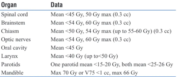
For the dosimetric evaluation of the treatment plan, DVHs are routinely used together with the mean dose of the dose distribution to the tumor planning target volume (PTV) and tolerance doses of the various tissues. Tolerance doses are usually given as the length of the irradiated portion of structure or fraction (volume) of the organ treated. These data are derived from patient observations and follow the conventional fraction schedule.[19,20]_{The dose constraints}

that were used for plan optimization in our study are given in Table 3.

Table 1: Sensitive organs at risks evaluated per patient

Patient# OARs

1 Mandible, larynx, spinal cord, brainstem, parotids 2 Mandible, larynx, spinal cord, brainstem, parotids 3 Mandible, larynx, spinal cord, brainstem, parotids 4 Mandible, larynx, spinal cord, parotids

5 Mandible, spinal cord, brainstem, parotids 6 Optic chiasm, brainstem, eyes, optic nerves 7 Larynx, brainstem, parotids, right orbit 8 Spinal cord, brainstem, parotids, orbits 9 Brainstem, optic chiasm, parotids

10 Brainstem, optic chiasm, orbits, optic nerves OAR: Organs at risk

Table 2: Prescription values per patient

Patient# Number of fractions Total dose (Gy)

1 33 69.96 2 35 70 3 35 70 4 33 69.96 5 30 60 6 32 64 7 33 70 8 30 60 9 35 70 10 35 70

(3)

In this study, linear-quadratic-Poisson model is used to describe the dose–response relations of the tumors and normal tissues: P D( ) exp ee D D e / ln ln = − −

(

)

⋅

(

−

)

        γ γ 50 2 ₍₁₎

where P(D) is the probability to control the tumor or induce a certain injury to a normal tissue that is irradiated uniformly with a dose D. D₅₀ is the dose which gives a 50% response, and γ is the maximum normalized dose–response gradient. Parameters D₅₀ and γ are organ and type of clinical endpoint specific and can be derived directly from clinical data.[12-14]

The response of a normal tissue to a nonuniform dose distribution is given by the relative seriality model which accounts for the volume effect. The dose–response parameters that were used in this study are based on the published data and presented in Table 4.[21]_{This study is assuming that the}

10 patients are of average radiosensitivity, thus characterized by the mean estimates of the radiobiological parameters presented.

Theory for applied methodology

Dosimetric evaluation does not take into account the biological characteristics of the tumor. Different solutions

to this problem have been recommended.[22-24]_{The article by}

Mavroidis et al.[10]_{generalized the mathematical expressions}

of D_eff[25]_{and EUD}[26]_{to deal with multiple target or normal}

tissue cases and introduced the BEUD concept. This is the dose that causes the same tumor control or normal tissue complication probability as the real dose distribution. This allows for the comparison of treatment plans based on the radiobiological endpoints by normalizing dose distributions to a common prescription point and plotting the tissue response probability versus D, which is given from the following analytical formula: P D P D D e P D e ( ) ( ) ln( ln( ( ))) ln(ln( ))   = ⇒ = − − − γ γ 2 (2)

The scalar quantity P₊, which expresses the probability of achieving tumor control without causing severe damage to normal tissue, can be estimated from the following mathematical expression:[8]

P+=P PB− B I∩ ≈P PB− I (3)

where P_B is the probability of getting benefit from treatment (tumor control) and P_I is the probability of causing severe injury to normal tissues (complications).

Statistical analysis

The different dose distributions of the study were radiobiologically evaluated using the radiation sensitivities of the tumors and OARs involved to calculate the probabilities of benefit and injury, as well as the values of complication-free tumor control probability P₊ and D.

Statistical analysis is done for P₊ clinical delivered values for the three cases – one-to-all, cascade, and planed values. Nonparametric statistical tests were used since they have no assumptions regarding distribution of underlying populations or variance. In view of the fact that our sample size is rather small (n = 10), several nonparametric tests for small samples were performed on the calculated data:

• The Mann–Whitney U-test • The sign test

• The Wilcoxon signed-rank test

• The Kendall tau rank correlation coefficient.

The Mann–Whitney U-test is used to decide whether or not there is a difference between the two groups. The groups compared were one-to-all versus planned values, cascade versus planned values, and one-to-all versus cascade values. The sign test was used to determine whether planned and CT-on-rails calculated data are different. The most accurate nonparametric test for paired data is the Wilcoxon signed-rank test. With this test, we test our null hypothesis that when it comes to calculated P₊ values, CT-on-rails data will produce worse results than the planned data. The Kendall tau rank correlation coefficient is used for nonparametric data and is used to measure the degree of correspondence between sets of rankings where the measures are not equidistant.

Table 3: Dose constraints for plan optimization for the various head‑and‑neck structures used for plan comparison

Organ Data

Spinal cord Mean <45 Gy, 50 Gy max (0.3 cc) Brainstem Mean <54 Gy, 60 Gy max (0.3 cc)

Chiasm Mean <50 Gy, 54 Gy max (up to 55-60 Gy) (0.3 cc) Optic nerves Mean <54 Gy, 60 Gy max (0.3 cc)

Oral cavity Mean <45 Gy

Larynx Mean <40 Gy (up to<50 Gy)

Parotids One parotid mean <15-20 Gy, both mean <25-26 Gy Mandible Max 70 Gy or V75 <1 cc, max 66 Gy

Table 4: Summary of the model parameter values used. The α/β was assumed to be 3 Gy for normal tissues and 10 Gy for the targets

Structure D₅₀ (Gy) γ s Endpoint

PTV 51.0 7.5 - Control

Spinal cord 57.0 6.7 1.00 Cervical myelopathy Parotid gland 46.0 1.8 0.01 Xerostomia

Mandible 70.3 3.8 1.00 Marked limitation of joint function Brainstem 65.1 2.4 1.00 Necrosis infarction

Brain 60.0 2.6 0.64 Necrosis infarction Larynx 78.8 4.8 0.66 Cartilage necrosis

Esophagus 62.3 2.0 0.11 Clinical stricture/perforation Oral cavity 70.0 3.0 0.50 Mucositis

Thyroid 90.0 2.0 0.1 Radiation-induced hypothyroidism Unspecified

normal tissue 65.0 2.3 1.00 Necrosis PTV: Planning target volume

(4)

r

esults

Graphical evaluation of the different plans

In Figure 1 (patient 9 example) and in Appendix Figures 1 and 2, the treatment plans are compared in terms of the DVH and BEUD of benefit (DB). The dose–response curves of each

target and OAR, together with the corresponding P₊ curves, are presented for the individual patients and plans. The dose–response curves are normalized to the D_B, which is forcing the response curves of the PTV (P_B) of the evaluated cases to coincide.

In Appendix Figures 1 and 2, more qualitative description of the comparison is presented. For most of the cases, it is shown that the treatment plan is satisfying plan objectives. In most cases, OAR is spared very well apart from a few that are located close to the PTV, left parotid for patient 1, larynx for patient 2, right parotid for patient 3, mandible for patients 4 and 5, left optic nerve for patient 6, right parotid for patient 7, optic chiasm for patient 9, and optic nerves for patient 10. Overall, the cascade case, when it comes to the PTV coverage, followed the plan values more closely than the one-to-all case, which is also visible from the plots in Appendix Figures 1 and 2. Plotting the curves of P_B, P_I, and P₊ of the three cases (plan, one-to-all, and cascade) on the same diagram shows that the corresponding curves of the PTVs (P_B) for the three cases coincide. In this situation, the response curves of the OAR (P_I) determine the difference in the plans that are compared, i.e., which case is superior from the radiobiological point of view. In these plots, P₊ is also used as an objective that depicts the quality of the cases being compared.

Quantitative summary of the dosimetric and radiobiological metrics

The values obtained for structures based on their tolerance doses [Table 3] are listed in Appendix Table 1. Based on those values, the differences between the planned and case values were calculated. In Appendix Tables 1-3, the quantitative summary of the physical and biological comparisons is

presented. The values (per patient and case) that represent the highest P₊ and the lowest P_I are highlighted in bold.

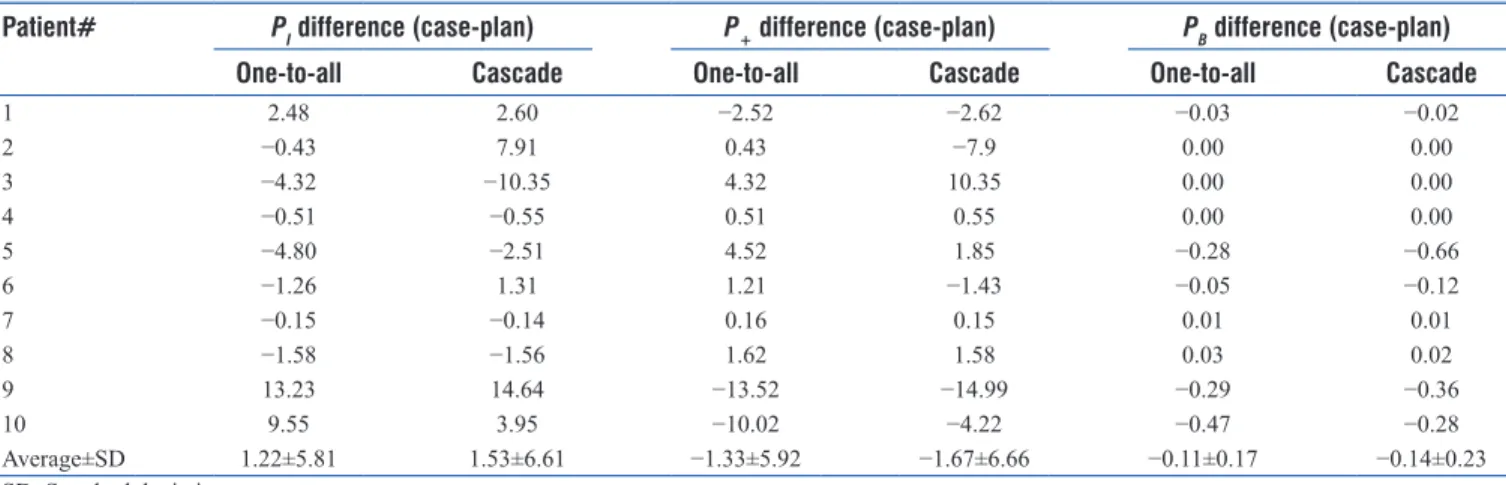
Table 5 lists the differences in P_B, P_I, and P₊ between each case and the planned values. The higher the value of the P_I difference, the higher is the P_I for the particular case (same goes for the P₊ and P_B comparison). The cascade case shows higher P_I values in 70% of the cases compared to the one-to-all case. The P_I plan values are lower than either of the cases in three patients out of ten. The dose variations in the PTV are listed in Table 6. The average percentage differences in minimum values were 3.23% and 3.11% for the one-to-all versus plan and cascade versus plan cases, respectively, and 0.49% and 0.57% in the maximum values, respectively.

For both analyzed cases, PTV coverage at the prescription dose and mean/maximum doses to the OAR are the same or slightly worse than it was in the plan [Appendix Table 1]. Average difference for the dosimetric values comparison of the “one-to-all” case to the planned values is 0.6 ± 1.8 Gy and for the “cascade” case to plan is 0.5 ± 1.8 Gy. When the patients are grouped in three groups based on the tumor location, the variation is 0.2 ± 0.4 Gy for both the “one-to-all” and “cascade” cases for the first group, 1.3 ± 3.3 Gy and 1.2 ± 3.4 Gy for the second group, respectively, and 0.2 ± 0.3 Gy for the third group, respectively. Table 6 shows that plans are not very homogeneous with some of the homogeneity actually improving with the one-to-all or cascade cases.

In Appendix Table 2, the clinical column indicates the biological effect calculated based on the prescribed dose delivered in the cases compared. The optimal column shows the corresponding highest achievable P₊ after dose escalation. Since the probability of achieving tumor control without causing severe damage to normal tissues is the pure benefit from the treatment (tumor control probability − normal tissue complication probability), in the case where the values of P_B are comparable, P₊ is going to be lower mainly due to the higher P_I. For the 10 patients, P₊ is lowest for the cascade case in the clinical column (in the 80% of cases total). Clinical standard for the overall P_I is usually set at 5%. Only for one patient, patient 4, P_I is at this acceptable level. Overall, the lowest P_I is present in the one-to-all cases. Higher overall P_I for the rest of cases stems from the significantly higher P(D) of the OAR for those cases, i.e., left parotid at 27.24% for cascade case versus 16.91% for the one-to-all case (patient 2), right parotid at 60.40% for the plan versus 55.61% for the one-to-all-case (patient 5), left eye at 37.28% for cascade case versus 33.57 for the one-to-all case (patient 6), brainstem at 5.79% for the plan versus 4.81% for the one-to-all case (patient 7), and left orbit at 7.40% for the plan versus 6.96% for the one-to-all case (patient 8). The P(D) of the other OARs is also higher in either cascade or plan cases versus the one-to-all case, contributing to the higher P_I in those cases.

Statistical analysis

The Mann–Whitney U-test was performed with a 95% degree of uncertainty (α = 0.05). The result is significant if Figure 1: The curves derived from the radiobiological evaluation of the

dose distributions are plotted, with the on the D_B dose axis. The solid line indicates the planned dose distribution, while the dashed line refers to the one‑to‑all case and the dotted line to the cascade case. These results correspond to patient 9

(5)

For the sign test, the result is significant if P < α. The 95% certainty required α = 0.05. For the comparison between the one-to-all and planned data, the calculated P is 0.344, and between the cascade and planned data, P = 1.246. This test showed that the result is not significant, and we can state that there is no difference between the planned and the CT-on-rails P₊ values.

In the Wilcoxon signed-rank test, the critical value of W for n = 10 and for a one-tailed test in which alpha = 0.05 equals 11. The null hypothesis can be rejected if test statistics W is greater than or equal to W critical. In our case, when the one-to-all data were compared with the planned data statistics, W was 25, and for the cascade versus planned data comparison, W was 31. Given that the test statistics W is greater than the critical W for both cases, null hypothesis is rejected, i.e., dosimetrically

(at least when comparing P₊ values), CT-on-rails data are not worse or better than the planned data.

The calculated Kendall tau rank correlation coefficient value for the one-to-all versus planned data was 0.911, for the cascade versus planned data was 0.867, and for the one-to-all versus cascade data was 0.956. High tau values indicate high degree of correspondence between the each group’s rankings.

d

IscussIon

In the physical analysis of the different dose distributions, criteria such as the mean and minimum target doses, mean and maximum normal tissue doses, isodose levels, and DVHs are mostly used.[27,28]_{The plans tried to achieve adequate PTV}

coverage while respecting the tolerance doses of the involved OAR. However, when comparing different dose distributions, the differences that are observed on the DVHs and isodose lines are not always reflected in the radiobiological evaluation. This is due to the fact that radiobiological evaluation is more sensitive to small changes in dose distribution that may often not be observed in the DVH-based evaluations.

The expected complication-free tumor control for the “planned,” “one-to-all,” and “cascade” dose distributions

Table 5: P values comparison (difference) of the “clinical” values between the two cases and the planned values

Patient# P_I difference (case‑plan) P₊ difference (case‑plan) P_B difference (case‑plan)

One‑to‑all Cascade One‑to‑all Cascade One‑to‑all Cascade

1 2.48 2.60 −2.52 −2.62 −0.03 −0.02 2 −0.43 7.91 0.43 −7.9 0.00 0.00 3 −4.32 −10.35 4.32 10.35 0.00 0.00 4 −0.51 −0.55 0.51 0.55 0.00 0.00 5 −4.80 −2.51 4.52 1.85 −0.28 −0.66 6 −1.26 1.31 1.21 −1.43 −0.05 −0.12 7 −0.15 −0.14 0.16 0.15 0.01 0.01 8 −1.58 −1.56 1.62 1.58 0.03 0.02 9 13.23 14.64 −13.52 −14.99 −0.29 −0.36 10 9.55 3.95 −10.02 −4.22 −0.47 −0.28 Average±SD 1.22±5.81 1.53±6.61 −1.33±5.92 −1.67±6.66 −0.11±0.17 −0.14±0.23 SD: Standard deviation

Table 6: Planning target volume dose variations per patient (Gy) with the deviations of the two cases from the plan

Patient# Plan Plan‑one‑to‑all Plan‑cascade

D_mean SD D₉₅ D_min D_max D_mean SD D₉₅ D_min D_max D_mean SD D₉₅ D_min D_max

1 64.61 6.17 68.22 53.92 75.28 0.17 0.09 0.09 0.00 0.33 0.18 0.02 0.08 0.12 0.22 2 72.2 3.48 73.69 66.17 78.22 −0.05 0.22 0.14 −0.44 0.34 −0.19 0.26 0.17 −0.64 0.27 3 69.03 5.78 72.68 59.03 79.01 0.29 0.12 0.05 0.1 0.48 0.43 0.18 0.07 0.12 0.74 4 69.44 2.72 68.79 64.74 74.03 0.31 −0.05 0.12 0.39 0.12 0.29 −0.03 0.14 0.35 0.13 5 52.93 6.34 57.81 41.96 63.88 0.17 0.01 0.13 0.17 0.18 0.53 −0.20 0.15 0.88 0.19 6 61.7 3.97 57.34 52.48 64.76 0.28 0.14 0.14 −0.04 0.39 0.35 0.17 0.15 −0.04 0.48 7 73.35 16.63 58.08 34.71 86.18 0.14 0.32 −0.06 −0.62 0.39 0.29 0.42 0.00 −0.69 0.61 8 52.32 2.45 54.12 48.07 56.55 0.04 0.00 −0.19 0.03 0.03 0.17 −0.08 −0.19 0.31 0.03 9 58 12.23 69.46 36.82 79.14 −4.59 2.96 0.19 −9.72 0.53 −3.89 2.77 0.24 −8.70 0.91 10 58.06 12.73 70.88 36.02 80.05 −0.48 0.85 0.37 −1.95 0.98 −0.19 0.57 0.21 −1.17 0.79 SD: Standard deviation

(6)

varies from case to case. For most of the studied cases, the planned dose distribution is better than the delivered dose distributions against either the one-to-all or cascade cases. The reason for this is the more effective irradiation of the PTV in the treatment plan, while normal tissue sparing is similar between the three compared distributions. However, even though in some cases the planned dose distribution may deliver lower mean doses to a given OAR, it may also show higher complication probability because of the greater maximum doses and higher seriality value of that OAR (e.g., spinal cord). Furthermore, the expected complication-free tumor control for the planned dose distributions is not always better than the delivered dose distributions for either cascade or one-to-all cases. The reason is that the different plans were not optimized using radiobiological objectives, which means that the planned dose distributions do not correspond to the maximum expected complication-free tumor control. It is observed that for normal tissues, the classification of the different dose distributions over the different cases seems to be more sensitive. In all the cases, the PTV is irradiated almost iso-effectively by the delivered dose distributions in one-to-all and the cascade cases. This is supported by the tumor control probabilities, P_B. On the other hand, the setup uncertainties produce higher normal tissue complications when the OARs move into the high-dose region (patients 3, 5, 6, and 8) or lower expected responses when the OARs move away from the high-dose region (patients 1, 2, 4, 7, 9, and 10).

The findings of this study indicate that for a fraction of the patients, the difference in expected outcome between the delivered against the planned doses can vary from 5% to 10%. For individual OARs, those values are even larger (up to 21%) [Appendix Table 3]. These results are in line with a recent study, which utilized head-and-neck cancer patients with daily CT-on-rails, where they report that, without altering patient setup, DVH analysis showed an increase in dose of 3%, 12%, and 16% to the tumor, cord, and parotids, respectively. With patient shifts to correct for setup errors, accurate dose delivery to the tumor was achieved. However, even with shifts, the cord and parotids were still overdosed by 10%.[29]_{Another study,}

using the IGRT results of five head-and-neck patients, reported that the impact of residual setup error, tumor shrinkage, organ deformation, or patient weight loss would result in a considerable change (up to 20%) in the dose received by the OARs.[30]

The statistical analysis of the P₊ values was done by means of various statistical tests, which showed that there is no statistically significant difference between the planned and the CT-on-rails P₊ values. This confirms the belief that if appropriate setup corrections are done on the patient, before each treatment, the delivered dose distribution is comparable to the planned dose distribution, regardless of how the CT-on-rail data from every fraction are grouped and analyzed.

It has to be stated that the determination of the model parameters expressing the effective radiosensitivity of the tissues is subject to uncertainties imposed by the inaccuracies

in the patient setup during RT, lack of knowledge of the inter-patient and intra-patient radiosensitivity, and inconsistencies in treatment methodology. Consequently, the determined model parameters (such as the D₅₀, γ, and s) and the corresponding dose–response curves are characterized by confidence intervals. In the present study, most of the tissue response parameters have been taken from recently published clinical studies.[12,14,15]

c

onclusIon

In this study, the clinical effectiveness of planned and delivered dose distributions of IMRT treatments for head-and-neck cancer was evaluated using both physical and biological criteria. The difference between the “one-to-all” and “cascade” dose distributions was small, statistically insignificant, and very close to the values of the corresponding treatment plans. However, for a fraction of the patients and given OAR, the differences between the delivered and planned doses were particularly large. These findings support the necessity of the accurate patient setup before the treatment using IGRT, thus minimizing dose delivery errors.

Acknowledgment

This research is supported by the Andrew Sabin Family Foundation; Dr. Fuller is a Sabin Family Foundation Fellow. Dr. Fuller receives funding and salary support from the National Institutes of Health (NIH), including: the National Institute for Dental and Craniofacial Research Award (1R01DE025248-01/ R56DE025248-01); a National Science Foundation (NSF), Division of Mathematical Sciences, Joint NIH/NSF Initiative on Quantitative Approaches to Biomedical Big Data (QuBBD) Grant (NSF 1557679); the NIH Big Data to Knowledge (BD2K) Program of the National Cancer Institute (NCI) Early Stage Development of Technologies in Biomedical Computing, Informatics, and Big Data Science Award (1R01CA214825-01); NCI Early Phase Clinical Trials in Imaging and Image-Guided Interventions Program (1R01CA218148-01); an NIH/NCI Cancer Center Support Grant (CCSG) Pilot Research Program Award from the UT MD Anderson CCSG Radiation Oncology and Cancer Imaging Program (P30CA016672) and an NIH/NCI Head and Neck Specialized Programs of Research Excellence (SPORE) Developmental Research Program Award (P50 CA097007-10). Dr. Fuller has received direct industry grant support and travel funding from Elekta AB and served as a consultant for Philips Medical Systems.

Financial support and sponsorship

Nil.

Conflicts of interest

There are no conflicts of interest.

r

eferences

1. Bel A, van Herk M, Bartelink H, Lebesque JV. A verification procedure to improve patient set-up accuracy using portal images. Radiother Oncol 1993;29:253-60.

(7)

profiles considering uncertainties in beam patient alignment. Acta Oncol 1993;32:331-42.

3. Creutzberg CL, Althof VG, Huizenga H, Visser AG, Levendag PC. Quality assurance using portal imaging: The accuracy of patient positioning in irradiation of breast cancer. Int J Radiat Oncol Biol Phys 1993;25:529-39.

4. ACR – ASTRO Practice Parameter for Image – Guided Radiation Therapy. Revised (CSC/BOC); 2014.

5. Jensen NK, Stewart E, Lock M, Fisher B, Kozak R, Chen J, et al. Assessment of contrast enhanced respiration managed cone-beam CT for image guided radiotherapy of intrahepatic tumors. Med Phys 2014;41:051905.

6. Sutton MW, Fontenot JD, Matthews KL 2nd_{, Parker BC, King ML,}

Gibbons JP, et al. Accuracy and precision of cone-beam computed tomography guided intensity modulated radiation therapy. Pract Radiat Oncol 2014;4:e67-73.

7. Yip C, Thomas C, Michaelidou A, James D, Lynn R, Lei M, et al. Co-registration of cone beam CT and planning CT in head and neck IMRT dose estimation: A feasible adaptive radiotherapy strategy. Br J Radiol 2014;87:20130532.

8. Källman P, Lind BK, Brahme A. An algorithm for maximizing the probability of complication-free tumor control in radiation therapy. Phys Med Biol 1992;37:871-90.

9. Mavroidis P, Stathakis S, Gutierrez A, Esquivel C, Shi C, Papanikolaou N,

et al. Expected clinical impact of the differences between planned and

delivered dose distributions in helical tomotherapy for treating head and neck cancer using helical megavoltage CT images. J Appl Clin Med Phys 2009;10:2969.

10. Mavroidis P, Lind BK, Brahme A. Biologically effective uniform dose (D) for specification, report and comparison of dose response relations and treatment plans. Phys Med Biol 2001;46:2607-30. 11. Brahme A. Which parameters of the dose distribution are best related to

the radiation response of tumours and normal tissues? In: Interregional Seminars for Europe, the Middle East and Africa Organized by the IAEA: Proceedings. Leuven; 1994. p. 37-58.

12. Emami B, Lyman J, Brown A, Coia L, Goitein M, Munzenrider JE, et al. Tolerance of normal tissue to therapeutic irradiation. Int J Radiat Oncol Biol Phys 1991;21:109-22.

13. Ågren AK. Quantification of the Response of Heterogeneous Tumors and Organized Normal Tissues to Fractionated Radiotherapy. Ph.D. Thesis. Stockholm University; 1995.

14. Mavroidis P, Laurell G, Kraepelien T, Fernberg JO, Lind BK, Brahme A,

et al. Determination and clinical verification of dose-response

parameters for esophageal stricture from head and neck radiotherapy. Acta Oncol 2003;42:865-81.

15. Mavroidis P, al-Abany M, Helgason AR, Agren Cronqvist AK, Wersäll P, Lind H, et al. Dose-response relations for anal sphincter regarding fecal leakage and blood or phlegm in stools after radiotherapy for prostate cancer. Radiobiological study of 65 consecutive patients. Strahlenther Onkol 2005;181:293-306.

16. Velocity AI. Velocity Medical Solutions. Available from: www.varian.com/ oncology/products/software/velocity. [Last accessed on 2018 Feb 13]. 17. Kessler ML. Image registration and data fusion in radiation therapy. Br

J Radiol 2006;79:S99-108.

18. Kadoya N, Fujita Y, Katsuta Y, Dobashi S, Takeda K, Kishi K, et al. Evaluation of various deformable image registration algorithms for thoracic images. J Radiat Res 2014;55:175-82.

19. Lyman JT. Tolerance Doses for Treatment Planning. Department of Energy, LBL-22416; 1985.

20. Bentzen SM, Constine LS, Deasy JO, Eisbruch A, Jackson A, Marks LB, et al. Quantitative analyses of normal tissue effects in the clinic (QUANTEC): An introduction to the scientific issues. Int J Radiat Oncol Biol Phys 2010;76:S3-9.

21. Mavroidis P, Ferreira BC, Papanikolaou N, Lopes Mdo C. Analysis of fractionation correction methodologies for multiple phase treatment plans in radiation therapy. Med Phys 2013;40:031715.

22. Ebert MA. Viability of the EUD and TCP concepts as reliable dose indicators. Phys Med Biol 2000;45:441-57.

23. Jones LC, Hoban PW. Treatment plan comparison using equivalent uniform biologically effective dose (EUBED). Phys Med Biol 2000;45:159-70.

24. Agren A, Brahme A, Turesson I. Optimization of uncomplicated control for head and neck tumors. Int J Radiat Oncol Biol Phys 1990;19:1077-85. 25. Brahme A. Dosimetric precision requirements in radiation therapy. Acta

Radiol Oncol 1984;23:379-91.

26. Niemierko A. Reporting and analyzing dose distributions: A concept of equivalent uniform dose. Med Phys 1997;24:103-10.

27. Aaltonen P, Brahme A, Lax I, Levernes S, Näslund I, Reitan JB, et al. Specification of dose delivery in radiation therapy. Recommendations by the Nordic Association of Clinical Physics (NACP). Acta Oncol 1997;36:1-32.

28. ICRU Report 62. Prescribing, Recording and Reporting Photon Beam Therapy (Supplement to ICRU Report 50). International Commission on Radiation Units and Measurements; 1999. p. 1-52.

29. Chen CP, Wong J, Chang CW, El-Gabry M, Merrick S, Gao Z. Plan degradation in head and neck cancers. Int J Radiat Oncol Biol Phys 2008;72:S592-3.

30. Lee L, Le QT, Xing L. Retrospective IMRT dose reconstruction based on cone-beam CT and MLC log-file. Int J Radiat Oncol Biol Phys 2008;70:634-44.

(8)

Appendix Figure 1: The dose–volume histograms of the planning target volume and the organs at risk are illustrated. The solid lines indicate the planned dose distributions, while the dashed lines correspond to the one‑to‑all case and the dotted lines to the cascade case

(9)

Appendix Figure 2: The curves derived from the radiobiological evaluation of the dose distributions are plotted using the D as the unit on the dose axis. The solid lines indicate the planned dose distributions, while the dashed lines correspond to the one‑to‑all case and the dotted lines to the cascade case

(10)

Appendix Table 1: Dosimetric value differences per patient per case (each case compared to planed values)

Patient Organ Dose Difference (Gy) Difference percentage PTV coverage

A B A B

Patient 1 Mandible Maximum −0.2 −0.1 −1.0 −1.0

Larynx Mean 0.0 0.0

Spinal cord Maximum 0.0 −0.1

Brainstem Maximum −0.1 −0.1

Left parotid Mean −0.1 0.0

Patient 2 Mandible Maximum −0.1 −0.1 0.0 0.0

Larynx Mean −0.4 −0.4

Spinal cord Maximum −0.1 0.0

Left parotid Mean 0.0 0.0

Patient 3 Mandible Maximum −0.3 −0.2 0.0 0.0

Larynx Mean −0.1 0.0

Spinal cord Maximum −0.2 −0.2

Right parotid Mean −1.7 −1.6

Spinal cord Maximum 0.1 0.0

Right parotid Mean 0.2 0.2

Brainstem Maximum 0.0 0.0

Left parotid Mean −0.3 −0.1

Patient 6 Optic chiasm Maximum −0.2 −0.2 −1.1 −1.2

Right eye Maximum 0.0 0.0

Right optic nerve Maximum 0.0 0.0

Patient 7 Brainstem Maximum −0.3 −0.1 0.0 −0.1

Right orbit Maximum −0.1 −0.3

Left parotid Mean 0.0 0.0

Patient 8 Brainstem Maximum 0.1 0.0 0.0 0.0

Left orbit Maximum −0.8 −0.8

Patient 9 Optic chiasm Maximum 1.1 1.3 −0.6 −0.7

Left parotid Mean −0.1 −0.1

Patient 10 Optic chiasm Maximum 11.7 11.8 −0.6 −0.4

Left orbit Maximum −0.5 −0.5

Left optic nerve Maximum 2.0 0.1

(11)

Appendix Table 2: Summary of the radiobiological comparison for the ten patients

Dose

prescription _ClinicalOne‑to‑all Cascade Plan Patient #

delivered deliveredOptimal deliveredClinical deliveredOptimal plannedClinical plannedOptimal

P+ (%) 78.8 96.0 78.7 96.2 81.3 97.0 1 PB (%) 99.9 97.7 100.0 97.9 100.0 98.4 PI (%) 21.2 1.8 21.3 1.8 18.7 1.4 BEUD-b (Gy) 68.2 60.3 68.5 60.5 69.6 61.1 BEUD-i (Gy) 42.1 35.8 42.1 35.8 41.6 35.5 P+ (%) 59.7 97.2 51.4 95.9 59.3 97.6 2 PB (%) 100.0 98.7 100.0 98.7 100.0 99.2 PI (%) 40.3 1.5 48.6 2.7 40.7 1.6 BEUD-b (Gy) 75.1 61.9 75.1 61.9 75.1 62.9 BEUD-i (Gy) 45.7 36.0 47.0 37.1 45.8 36.0 P+ (%) 9.9 67.3 15.9 69.3 5.6 43.7 3 PB (%) 100.0 91.4 100.0 91.4 100.0 91.4 PI (%) 90.1 24.1 84.1 22.1 94.4 47.7 BEUD-b (Gy) 74.3 57.8 74.3 57.8 74.4 57.8 BEUD-i (Gy) 55.6 43.2 53.7 42.8 57.5 46.9 P+ (%) 94.5 99.4 94.5 99.4 94.0 99.4 4 PB (%) 100.0 99.7 100.0 99.7 100.0 99.7 PI (%) 5.5 0.3 5.4 0.3 6.0 0.3 BEUD-b (Gy) 70.8 64.7 70.8 64.7 70.9 64.7 BEUD-i (Gy) 38.1 33.0 38.1 33.0 38.3 33.1 P+ (%) 41.2 46.9 38.5 43.5 36.7 42.8 5 PB (%) 97.0 87.4 96.7 90.7 97.3 88.0 PI (%) 55.9 40.5 58.2 47.2 60.7 45.3 BEUD-b (Gy) 58.9 55.7 58.7 56.4 59.1 55.9 BEUD-i (Gy) 46.3 44.1 46.7 45.1 47.0 44.8 P+ (%) 44.6 53.0 42.0 49.8 43.4 51.7 6 PB (%) 97.7 91.0 97.7 91.2 97.8 91.1 PI (%) 53.1 38.1 55.7 41.4 54.4 39.4 BEUD-b (Gy) 60.1 57.0 60.0 57.0 60.1 57.0 BEUD-i (Gy) 45.4 42.5 45.9 43.2 45.7 42.7 P+ (%) −6.3 0.0 −6.3 0.0 −6.5 0.0 7 PB (%) 92.2 0.0 92.2 0.0 92.1 0.0 PI (%) 98.5 0.0 98.5 0.0 98.6 0.0 BEUD-b (Gy) 66.4 0.0 66.4 0.0 66.4 0.0 BEUD-I (Gy) 58.1 0.5 58.1 0.5 58.4 0.5 P+ (%) 63.5 70.3 63.4 70.2 61.9 68.5 8 PB (%) 84.1 97.0 84.1 97.0 84.1 97.0 PI (%) 20.6 26.8 20.7 26.8 22.2 28.6 BEUD-b (Gy) 55.2 58.9 55.2 58.9 55.2 58.9 BEUD-i (Gy) 36.0 37.5 36.0 37.5 36.4 37.8 P+ (%) 8.6 49.0 7.2 48.0 22.2 54.9 9 PB (%) 76.9 54.1 76.8 54.1 77.2 58.2 PI (%) 68.2 5.2 69.7 6.1 55.0 3.3 BEUD-b (Gy) 73.3 66.7 73.3 66.7 73.4 67.7 BEUD-i (Gy) 50.1 38.5 50.4 38.9 48.0 37.5 P+ (%) 10.1 18.4 15.9 22.3 20.1 24.5 10 PB (%) 78.8 57.9 79.0 61.7 79.3 65.4 PI (%) 68.7 39.5 63.1 39.4 59.2 41.0 BEUD-b (Gy) 74.0 67.6 74.1 68.6 74.2 69.6 BEUD-i (Gy) 49.0 43.7 48.1 43.6 47.5 44.0

(12)

Appendix Table 3: Quantitative summary of the biological comparison for the dose distributions of the ten cases

P‑0

(%) (%)P‑1 (%)P‑2 BEUD‑0 (Gy) BEUD‑1 (Gy) BEUD‑2 (Gy) _(Gy)D‑0 _(Gy)D‑1 _(Gy)D‑2 SD‑0 (Gy) SD‑1 (Gy) SD‑2 (Gy)

Patient 1 s PTV 99.97 99.94 99.95 69.55 68.15 68.50 71.20 71.12 71.13 1.65 1.82 1.78 Mandible 11.04 13.75 13.79 63.65 64.15 64.15 42.57 43.32 43.32 16.21 16.68 16.69 Larynx 0.32 0.28 0.46 66.30 66.20 66.55 29.73 29.82 32.75 25.32 24.98 26.22 Cord 0.00 0.00 0.00 49.70 49.70 49.70 27.03 26.50 26.08 11.04 10.15 10.50 Brainstem 0.00 0.00 0.00 41.90 41.85 41.85 27.22 27.11 27.16 13.30 13.23 13.18 Left parotid 8.29 8.34 8.26 41.05 41.05 41.05 37.09 37.15 37.12 24.05 23.92 23.93 Right parotid 0.00 0.00 0.00 17.55 17.65 17.65 15.89 15.99 15.98 10.78 10.76 10.76 Patient 2 PTV 100.0 100.0 100.0 75.10 75.05 75.05 75.26 75.22 75.22 0.84 0.86 0.87 Mandible 5.14 8.70 5.12 64.20 63.20 63.20 41.69 40.81 40.81 14.41 13.51 13.51 Larynx 20.99 21.80 25.52 72.95 72.85 73.40 49.94 49.96 52.44 29.64 29.31 29.09 Cord 0.00 0.00 0.00 50.45 50.45 50.45 30.78 35.32 36.08 15.15 11.03 10.16 Brainstem 0.00 0.00 0.00 38.05 39.65 39.40 11.46 13.80 13.76 12.94 14.78 14.73 Left parotid 20.29 16.91 27.24 44.30 45.15 46.75 39.21 40.10 41.68 28.14 28.24 28.63 Right parotid 0.00 0.01 0.00 29.70 28.65 27.55 26.39 25.46 24.49 19.04 18.43 17.75 Patient 3 PTV 100.0 100.0 100.0 74.35 74.30 74.30 75.02 74.98 74.98 1.25 1.24 1.24 Cord 0.00 0.00 0.00 50.45 50.45 50.45 30.16 32.88 33.34 13.44 10.76 11.01 Brainstem 0.00 0.00 0.00 42.20 42.15 42.05 34.36 34.15 33.94 5.51 5.79 5.96 Larynx 0.00 0.00 0.00 57.15 57.15 57.15 30.13 33.04 29.35 15.10 14.82 14.88 Mandible 29.41 50.35 25.80 67.55 70.30 67.05 51.80 57.96 51.01 15.29 16.91 14.84 Right parotid 91.93 80.09 78.55 66.00 59.55 58.95 64.75 57.87 57.28 16.76 18.91 18.91 Left parotid 2.31 0.02 0.02 38.15 30.80 30.80 34.72 26.89 26.88 21.68 21.24 21.26 Patient 4 PTV 99.98 99.98 99.98 70.90 70.80 70.80 71.29 71.22 71.21 1.23 1.24 1.24 Cord 0.00 0.00 0.00 49.70 49.70 49.70 26.20 29.94 29.95 12.16 9.10 9.04 Larynx 1.68 1.29 1.24 67.70 67.45 67.40 32.10 32.18 32.21 23.27 22.58 22.42 Mandible 4.39 4.25 4.25 61.95 61.90 61.90 46.23 46.21 46.21 15.44 15.37 15.37 Right parotid 0.00 0.00 0.00 27.35 27.35 27.35 24.03 24.07 24.10 18.38 18.21 18.13 Left parotid 0.00 0.00 0.00 24.10 24.10 24.10 21.50 21.51 21.57 15.31 15.24 15.07 Patient 5 PTV 97.31 97.03 96.65 59.10 58.90 58.65 60.67 60.62 60.61 1.49 1.53 1.54 Brainstem 0.00 0.00 0.00 33.35 33.35 33.35 25.08 25.01 25.02 4.76 4.79 4.78 Left parotid 0.50 0.42 0.40 34.10 33.85 33.80 29.17 29.01 28.98 24.05 23.68 23.62 Right parotid 60.40 55.61 57.92 51.70 50.65 51.15 49.64 48.54 49.08 18.62 18.80 18.65 Mandible 0.15 0.14 0.13 56.85 56.75 56.75 52.49 52.47 52.46 4.24 4.17 4.20 Cord 0.00 0.00 0.00 48.50 48.50 48.50 27.89 27.88 28.28 2.90 2.94 3.04 Patient 6 PTV 97.79 97.74 97.67 60.10 60.05 59.95 61.24 61.20 61.08 2.13 2.15 2.09 Chiasm 2.46 2.32 2.25 43.45 43.35 43.30 27.23 27.19 27.17 36.11 35.93 35.86 Brainstem 0.00 0.00 0.00 33.80 33.80 33.80 9.30 9.07 9.28 4.99 4.68 4.94 Left eye 35.70 33.57 37.28 48.35 47.55 48.90 41.20 40.46 41.97 17.50 17.14 17.45 Right eye 0.00 0.00 0.00 3.30 3.30 3.30 2.91 2.92 2.92 1.24 1.23 1.23

Left optic nerve 27.25 27.73 27.70 52.80 52.90 52.90 52.76 52.84 52.84 0.00 0.00 0.00

Right optic nerve 0.00 0.00 0.00 3.75 3.80 3.80 3.67 3.74 3.73 0.00 0.00 0.00

Patient 7 PTV 92.14 92.15 92.15 66.40 66.40 66.40 70.48 70.44 70.46 6.52 6.48 6.49 Larynx 0.00 0.00 0.00 58.30 57.45 57.95 17.57 17.74 17.70 11.80 11.63 11.65 Brainstem 5.79 4.81 4.96 55.35 54.90 54.95 46.10 45.47 45.54 11.68 11.53 11.52 Right orbit 13.29 13.18 13.18 39.10 39.00 39.00 34.91 34.79 34.91 9.48 9.51 9.40 Left parotid 0.00 0.00 0.00 20.65 20.70 20.70 18.92 18.96 18.95 11.86 11.84 11.84 Contd...

(13)

Appendix Table 3: Contd...

P‑0

(%) (%)P‑1 (%)P‑2 BEUD‑0 (Gy) BEUD‑1 (Gy) BEUD‑2 (Gy) _(Gy)D‑0 _(Gy)D‑1 _(Gy)D‑2 SD‑0 (Gy) SD‑1 (Gy) SD‑2 (Gy)

Right parotid 98.30 98.14 98.14 74.50 74.00 74.00 74.41 73.90 73.91 4.75 4.29 4.34 Patient 8 PTV 84.07 84.10 84.09 55.15 55.20 55.15 55.26 55.25 55.25 0.64 0.58 0.58 Brainstem 0.00 0.00 0.00 35.65 35.50 35.65 27.23 26.65 27.22 5.95 5.65 5.95 Cord 0.00 0.00 0.00 48.50 48.50 48.50 29.61 30.35 30.38 4.60 4.56 4.73 Left orbit 7.40 6.96 6.99 34.45 34.10 34.10 20.47 20.61 20.59 14.71 14.41 14.43 Left parotid 0.00 0.00 0.00 17.80 17.95 18.00 16.57 16.70 16.74 9.21 9.20 9.20 Right parotid 0.00 0.00 0.00 21.95 22.05 22.05 20.00 20.13 20.13 12.62 12.58 12.58 Right orbit 16.00 14.69 14.69 39.65 39.00 39.00 26.97 26.88 26.88 17.25 16.68 16.68 Patient 9 PTV 77.18 76.89 76.82 73.35 73.25 73.25 73.83 73.72 73.69 2.37 2.39 2.41 Brainstem 1.55 2.51 1.52 53.30 54.25 53.25 34.88 35.87 34.85 12.39 13.17 12.34 Chiasm 54.25 67.38 69.14 55.05 56.00 56.15 52.03 53.16 53.35 11.75 11.82 11.83 Left parotid 0.12 0.12 0.12 33.15 33.15 33.15 30.15 30.20 30.20 19.34 19.23 19.20 Right parotid 0.00 0.00 0.00 6.50 6.50 6.50 6.34 6.33 6.34 2.28 2.28 2.28 Patient 10 PTV 79.29 78.82 79.01 74.20 74.00 74.10 74.76 74.61 74.67 2.36 2.44 2.42 Brainstem 0.00 0.00 0.00 34.45 34.45 34.45 22.73 22.71 22.71 4.61 4.59 4.58 Chiasm 0.01 8.23 8.59 38.05 46.90 47.05 36.98 39.39 39.26 4.17 9.98 10.21 Left orbit 28.19 27.92 27.81 46.50 46.40 46.35 34.88 35.14 35.00 19.79 19.46 19.51 Right orbit 20.10 20.25 19.85 43.05 43.10 42.95 30.66 31.27 30.92 18.14 17.82 17.85 Left optic nerve 17.90 27.29 18.57 52.20 54.05 52.35 52.13 53.95 52.27 4.49 4.84 4.42 Right optic nerve 13.35 18.48 14.40 51.20 52.35 51.45 51.06 52.23 51.32 5.33 5.24 5.29 One-to-all case is represented by number “1,” cascade by number “2,” and planned values by “0.” PTV: Planning target volume, SD: Standard deviation