Performance of static and adpative subchannel allocation schemes for fractional frequency reuse in WiMAX networks

PERFORMANCE OF STATIC AND ADAPTIVE SUBCHANNEL

ALLOCATION SCHEMES FOR FRACTIONAL FREQUENCY REUSE

IN WiMAX NETWORKS

A THESIS

SUBMITTED TO THE DEPARTMENT OF ELECTRICAL AND ELECTRONICS ENGINEERING

AND THE GRADUATE SCHOOL OF ENGINEERING AND SCIENCES OF BILKENT UNIVERSITY

IN PARTIAL FULFILLMENT OF THE REQUIREMENTS FOR THE DEGREE OF

MASTER OF SCIENCE

By

GORKEM KAR July 2011

I certify that I have read this thesis and that in my opinion it is fully adequate, in scope and in quality, as a thesis for the degree of Master of Science.

Assoc. Prof. Dr. Ezhan Kara¸san (Supervisor)

I certify that I have read this thesis and that in my opinion it is fully adequate, in scope and in quality, as a thesis for the degree of Master of Science.

Assoc. Prof. Dr. Nail Akar

I certify that I have read this thesis and that in my opinion it is fully adequate, in scope and in quality, as a thesis for the degree of Master of Science.

Assistant Prof. Dr. Ka˘gan G¨okbayrak

Approved for the Graduate School of Engineering and Sciences:

Prof. Dr. Levent Onural

ABSTRACT

PERFORMANCE OF STATIC AND ADAPTIVE

SUBCHANNEL ALLOCATION SCHEMES FOR FRACTIONAL

FREQUENCY REUSE IN WiMAX NETWORKS

G¨orkem Kar

M.S. in Electrical and Electronics Engineering Supervisor: Assoc. Prof. Dr. Ezhan Kara¸san

July 2011

We study the downlink performance of WiMAX under fractional frequency reuse (FFR) model. Conventional cellular planning methods can be used for broadband wireless access systems that operate in point-to-multipoint (PMP) configuration based on OFDMA/OFDM such as WiMAX. As an alternative planning method, FFR has been recently proposed for OFDMA/OFDM based cellular systems. FFR divides the cell into two regions: the inner and outer cell. Mobile Stations (MS) inside the inner cell can use the entire frequency band (achieving full frequency reuse), while MSs in the outer ring use a fraction of the band (having fractional frequency reuse). Transmissions in the inner and outer cells occur during different time periods so that users at the cell edge experience less interference. In this thesis, we investigate the effect of dynamically changing the number of subcarriers allocated to inner and outer cells. We use two metrics: total cell throughput and Jain’s fairness index for the distribution of cell throughput among MSs. As the ratio of subcar-riers allocated to inner cell increases, the total cell throughput increases while the fairness index decreases. We use the product of cell throughput and fairness index in order to study the trade-off between the two metrics. We show that by dynamically adjusting the ratio of subcarriers allocated to the inner cell based on the user distribution, the

throughput-fairness index product can be increased by about 5% compared with the fixed optimum subcarrier allocation.

¨

OZET

WiMAX S

¸EBEKELER˙INDE KISM˙I FREKANS TEKRAR

KULLANIMI ˙IC

¸ ˙IN STAT˙IK VE AYARLANAB˙IL˙IR ALT

KANAL TAHS˙IS S

¸EMALARININ PERFORMANSI

G¨orkem Kar

Elektrik ve Elektronik M¨uhendisli˘gi B¨ol¨um¨u Y¨uksek Lisans Tez Y¨oneticisi: Do¸c. Dr. Ezhan Kara¸san

Temmuz 2011

Bu tezde, kısmi frekans tekrar kullanım modeli altında WiMAX performansını inceledik. Geleneksel h¨ucresel planlama y¨ontemleri, WiMAX gibi OFDMA/OFDM’ye dayalı, nok-tadan ¸cok noktaya d¨uzenle¸sim (PMP) yapılandırmayla ¸calı¸san geni¸s bant kablosuz eri¸sim sistemleri i¸cin kullanılabilir. Son zamanlarda, alternatif bir planlama y¨ontemi olarak FFR, OFDMA/OFDM tabanlı h¨ucresel sistemler i¸cin tasarlanmı¸stır. FFR h¨ucreyi i¸c ve dı¸s h¨ucre olmak ¨uzere 2 par¸caya ayırır. ˙I¸c h¨ucre i¸cindeki kullanıcılar (MS) t¨um frekans bandını kul-lanabilirken (tam frekans yeniden kullanımı), dı¸s h¨ucredeki kullanıcılar frekans bandının belirli bir kısmını (kısmi frekans kullanımı) kullanabilirler. ˙I¸c ve dı¸s h¨ucredeki iletimler farklı zaman dilimlerinde ger¸cekle¸sir b¨oylece h¨ucre kenarında bulunan kullanıcılar daha az parazitle kar¸sıla¸sırlar. Bu tezde, i¸c ve dı¸s h¨ucredeki kullanıcılara ayrılan alt ta¸sıyıcı sayısının etkilerini inceledik. Toplam h¨ucre verimlili˘gi ve Jain e¸sitlik indisi olmak ¨uzere 2 ¨ol¸c¨ut kul-landık. ˙I¸c h¨ucreye ayrılan altkanal oranı arttık¸ca, toplam h¨ucre verimlili˘ginin arttı˘gını, e¸sitlik indisinin ise azaldı˘gını g¨ozlemledik. Bu 2 ¨ol¸c¨ut arasındaki ili¸skiyi g¨ormek i¸cin h¨ucre verimlili˘gi ile e¸sitlik indisinin ¸carpımını inceledik. Kullanıcıların da˘gılımına g¨ore i¸c h¨ucreye ayrılan altkanal oranını dinamik olarak ayarlayarak, sabit ideal altkanal atamasına g¨ore verimlilik-e¸sitlik indisi ¸carpımında yakla¸sık %5’lik bir artı¸s g¨ozlemledik.

Acknowledgements

I would like to express my deep-felt gratitude to my advisor, Assoc. Prof. Dr. Ezhan Kara¸san of the Electrical and Electronics Department at Bilkent University, for his advice, encouragement, enduring patience and constant support. He always provided clear expla-nations when I was lost, and always giving me his time, in spite of anything else that was going on. I wish all students the honor and opportunity to experience his ability to perform at that job.

I also wish to thank the other members of my committee, Assoc. Prof. Dr. Nail Akar of the Electrical and Electronics Department and Assistant Prof. Dr. Ka˘gan G¨okbayrak of In-dustrial Engineering Department, both at Bilkent University. Their suggestions, comments and additional guidance were invaluable to the completion of this work.

I would like to thank Ahmet Serdar Tan for writing the initial version of the system level simulator and to Ozan Basciftci for the help in the improving part of the system level simulator. Without Ozan, it would be much thougher to implement FFR process.

Additionally, I want to thank to Electrical and Electronics Department professors and staff for all their hard work and dedication, providing me the means to complete my degree and prepare for an academic career. This includes (but certainly is not limited to) the following individuals:

Assistant Prof. Sinan Gezici

He made it possible for me to have many wonderful experiences I enjoyed while a student, including the opportunity to be teaching assistantship in the Telecom-munication class. He is one of my reasons to want to be an academician. Dr. Aydan Pamir

During my freshman year at Bilkent University, she taught me many things about calculus and life. For 4 semesters, I have experinced gradership experi-ence with her and it lead me to idea that become an academician. I wish all freshman students the opportunity to experience her academical knowledge and her kindness.

I am very grateful to my parents who have always given me their unconditional caring and support.

Table of Contents

List of Tables . . . xiii

1 Introduction . . . 1

2 WiMAX System Description . . . 8

2.1 WiMAX Frame Structure . . . 8

2.1.1 Subchannelization . . . 8

2.1.2 Frame Structure . . . 9

2.2 Adaptive Modulation and Coding . . . 11

2.3 Scheduling . . . 12

2.3.1 Proportional Fair (PF) Scheduling . . . 12

2.3.2 Fairness . . . 13

3 System Level Simulation of WiMAX . . . 14

3.1 Frequency Reuse Models . . . 14

3.1.1 Fractional Frequency Reuse . . . 15

3.2 Simulation Methodology . . . 18

3.2.1 Configuration . . . 19

3.2.2 Initialization . . . 20

3.3 Simulation Procedure and Flow . . . 21

3.3.1 Metric Computation . . . 21

3.3.2 Analysis . . . 23

4 Performance Evaluation of Static and Adaptive FFR . . . 24

4.1.1 Subchannel Allocation with Respect to Sector Areas . . . 27

4.1.2 Subchannel Allocation with Respect to User Distribution Under Mo-bility . . . 33

4.1.3 Throughput vs. Fairness . . . 38

4.2 Adaptive FFR . . . 42

5 Conclusions . . . 46

List of Figures

1.1 WiMAX Scenario [4] . . . 1

1.2 Frequency reuse patterns . . . 2

1.3 Illustration of FFR . . . 3

1.4 Illustration of FFR used in [8] . . . 4

1.5 DL subframe for FFR scheme . . . 5

1.6 Illustration of adaptive FFR . . . 6

2.1 OFDMA symbol structure in WiMAX [12] . . . 9

2.2 WiMAX frame structure [15] . . . 10

3.1 Frequency reuse patterns . . . 15

3.2 Illustration of FFR . . . 16

3.3 CDF of section throughput . . . 17

3.4 Illustration of FFR used in [8] . . . 17

3.5 Cellular deployment . . . 20

4.1 Frequency reuse patterns . . . 25

4.2 Illustration of the FFR . . . 25

4.3 DL subframe for FFR scheme . . . 26

4.4 Illustration of adaptive FFR . . . 26

4.5 Circular figure . . . 28

4.6 CDF of user throughput . . . 29

4.7 CDF of sector throughput . . . 29

4.8 Average user throughput vs. distance . . . 30

4.9 Burst profile histograms for FFR with r=0.4 . . . 32

4.10 Burst profile histograms for FFR with r=0.6 . . . 32

4.11 Burst profile histograms for FFR with r=0.8 . . . 33

4.12 Burst profile histograms for 1x3x3 . . . 33

4.14 CDF of user average packet retransmission . . . 34

4.15 RWP model illustrated . . . 35

4.16 CDF of user throughput for RWP . . . 36

4.17 CDF of sector throughput for RWP . . . 37

4.18 Average user throughput vs. distance for rwp . . . 37

4.19 Weighted throughput vs. fairness index . . . 38

4.20 Weighted throughput vs inner cell resource percentage for different ρ values 40 4.21 Fairness index vs inner cell resource percentage for different ρ values . . . . 40 4.22 Fairness index × throughput for different inner cell resource percentages . 41

List of Tables

2.1 OFDMA paramaters . . . 10

2.2 Supported codes and modulations in WiMAX . . . 11

2.3 PHY layer data rate at channel bandwidths 10 MHz . . . 11

3.1 OFDMA parameters . . . 18

3.2 System level simulator parameters . . . 19

3.3 Input parameters . . . 20

4.1 Default input parameters . . . 24

4.2 Percentage of inner cell users to all users for different inner radiuses . . . . 28

4.3 Percentage of inner cell users to all users for different inner radiuses . . . . 35

4.4 Throughput × fairness index for various frequency reuse patterns . . . 42

4.5 Frame number vs number of inner cell users . . . 43

4.6 Throughput × fairness index for fixed inner cell resources . . . 43

4.7 Throughput × fairness index for dynamic inner cell resources . . . 44

Chapter 1

Introduction

Worldwide Interoperability for Microwave Access (WiMAX) is one of the telecommuni-cation protocols designed to offer broadband mobile wireless access to multimedia and Internet applications [1]. Typical WiMAX scenario can be seen in Figure 1.1. The IEEE 802.16e standard [2] defines the technical features of the communications protocol includ-ing thes Medium Access Control (MAC) layer and physical layer of WiMAX. The WiMAX Forum [3] is an industry-led, not-for-profit organization formed to certify and promote the compatibility and interoperability of broadband wireless products based upon the harmo-nized IEEE 802.16/ETSI HiperMAN standard.

Figure 1.1: WiMAX Scenario [4]

The WiMAX physical layer is based on Orthogonal Frequency Division Multiplexing (OFDM). OFDM is a transmission scheme where a high rate data stream is divided into a parallel set of low rate substreams which are simultaneously transmitted. WiMAX uses

Orthogonal frequency division muliple access (OFDMA) to accommodate many users in the same channel at the same time. In WiMAX terminology, a subchannel means a group of subcarriers together by specific methods as defined in the standard. Subchannels represent the minimum granularity for allocation of frequency resources [5]. Subchannels are allocated to users by base stations (BSs). In order to allow users to transmit and receive at the same time, OFDMA distributes subcarriers within a single channel that are called subchannels which are used to decrease the effect of interference based on distance and propogation effects of each user.

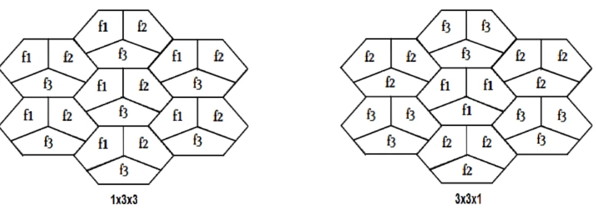
WiMAX is typically deployed as a cellular network. Each cell in the network has a hexagonal structure and has a single BS which is basically a router that communicates with mobile stations (MS) based on WiMAX standard, in the center. A cell is divided into a number of sectors (typically 3) in order to increase frequency reuse by reducing interference to other cells and sectors. A directional antenna is placed at the BS for each sector in the cell. Two exemplary frequency reuse patterns are shown in Figure 1.2. In the 1x3x3 reuse mode, each cell in the network is assigned whole spectrum but the whole spectrum is divided into three segments, namely f1, f2, and f3, and each sector in a particular cell is assigned only one of the segments. In 3x3x1 reuse mode, the whole spectrum band is divided into three segments, namely f1, f2, and f3 and each cell is assigned only one of the segments. Sectors in a particular cell are assigned the same segment.

Figure 1.2: Frequency reuse patterns

Fractional frequency reuse (FFR) is a recently proposed technique which divides the cell into two regions: the inner cell and outer cell. Since the inner cell users are closer to

the BS compared to the outer cell users, they are immune to co-channel interference so they use the entire frequency band, while users (MSs) in the outer cell use a fraction of the frequency band. Transmission in the inner and outer cells occur during different time periods so that users at the cell edge experience less interference.

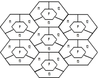
Figure 1.3 shows the network deployment for the FFR model that will be studied in this thesis. In FFR, each cell in the network is assigned the whole spectrum but for the outer cell, whole spectrum is divided into three segments, namely f1, f2, and f3, and each sector in outer cell is assigned only one of the segments. MSs inside the inner cell use the entire frequency band (F).

Figure 1.3: Illustration of FFR

In FFR method, cell edge users can get special treatment (by allocating more resources) to bring better signal quality. FFR maximizes spectral efficiency for users at the inner cell (with full frequency reuse) and improves signal quality and throughput for users at a cell edge.

FFR in the context of OFDMA systems has mainly been discussed in cellular network standardization forum such as Third Generation Partnership Project (3GPP) [6] and Third Generation Partnership Project 3 (3GPP2) [7]. In [8], the cell is divided into two regions as inner cell and outer cell and it adaptively assigns subcarriers to different sectors and the

whole spectrum band is divided into three segments, namely f1, f2, and f3 and each sector in the outer cell is assigned the same segment, for the inner cell the whole frequency band is used. An illustration of the FFR used in [8] can be seen in Figure 1.4. In this thesis, we also investigate the effect of dynamically changing the number of subcarriers allocated to inner and outer cells but in our case the sectors in the outer cell use different segments. By this method, outer cell users experience less interference since the adjacent sectors use different frequency segments.

Figure 1.4: Illustration of FFR used in [8]

In [9] and in [10], subcarrier allocation of sectors is same with the case we use in this thesis. In [9], they describe an algorithm for subcarrier and power allocation that achieves out-of-cell interference avoidance through dynamic FFR in downlink of cellular systems based on OFDMA. Their approach is based on each sector constantly performs optimization of the assignment of its users to resource sets, with the objective of optimizing its own performance. They use dynamical assigning of subcarriers in order to minimize power usage. In [10], an algorithm is proposed that adjust the tranmit powers of different subbands (used in different sectors of the cell) in order to maximize the overall network utility. The total power within each sector is upper bounded. In [9] and in [10], they concentrate on power usage of each user but we concentrate on the cell throughput and the distribution of the throughput among MSs.

in evaluating the performance of frequency reuse schemes. In traditional frequency reuse techniques (i.e, 1x3x3, 3x3x1), MSs that are close to cell edge experience unacceptable level of interference since they are distant to corresponding BS and this causes low throughput for these users. Since each MS in a cell has the same right to communicate, each MS should have a good quality of service and there shouldn’t be much difference in their signal quality in order to maintain number of happy customers. For this, we need to make sure that the throughput of each MS should be similar to each other. For this purpose, we use Jain’s fairness index which measures how the throughput is shared among users. Fairness index is maximum (equal to 1), when the throughput of each connection is same (all users receive the same allocation).

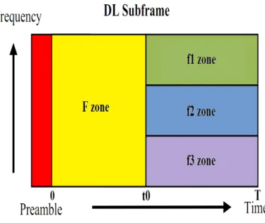
In Figure 1.5, we can see the DL subframe for FFR scheme. In this figure; F zone is the sum of all subchannels available and is used by inner cell users, f1, f2 and f3 are fractions of all subchannels available and is used by the outer cell sectors. Since we use 120◦ sectoring in FFR, f1, f2 and f3 are equal to each other. When we increase the F zone, we have much better throughput performance for the inner cell users but in return there is not enough subcarriers for users that are in outer cell sectors so the fairness index becomes worse. We use the multiplication of cell throughput and fairness index in order to study the trade-off between the two metrics.

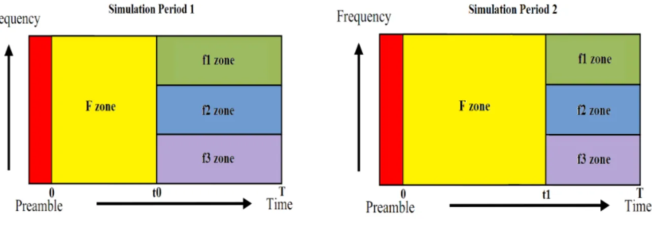
One of the key factors determining the FFR performance is how to assign subcarriers to users in order to get higher throughput and fairness index. We assign the subcarriers to the users both statically and adaptively. In static FFR, as shown in Figure 1.5, we fix frequency reuse zones (F, f1, f2 and f3) and allocate subcarriers to each user from the subset of subcarriers assigned to the zone corresponding to the location of the MS. In adaptive FFR, we start with a subcarrier allocation and we adjust the ratio of subcarriers allocated for the inner cell over time. In Figure 1.6, in simulation period 1 we start with a specific subcarrier allocation but in simulation period 2, we changed the allocation and increase the duration of F zone where t1 > t0 in order to increase the multiplication of total cell throughput and fairness index.

Figure 1.6: Illustration of adaptive FFR

In static FFR, we allocate subcarriers with respect to sector areas and with respect to user distribution under mobility. In subcarriers allocation with respect to sector areas, we assign subcarriers to inner and outer areas in proportion with the area of regions. In sub-carriers allocation with respect to user distribution under mobility, subsub-carriers are allocated based on the expected number of users within the sectors. In order to calculate the distri-bution of users, we use the Random Waypoint (RWP) model which is designed to describe the movement pattern of mobile users, and how their location, velocity and acceleration change over time [11]. In static allocation, we observe that when the throughput of the network increases, the fairness index decreases. In order to combine these two performance metrics into a single metric, we use the throughput-fairness index product and study the trade-off between the two metrics. When the inner cell user percentage changes over time,

we observe that by changing the ratio of subcarriers allocated for the inner cell, we can have better fairness × throughput performance. Since we adjust the ratio of subcarriers allocated for the inner cell over time, we call this method adaptive FFR. By assigning the subcarriers to the users adaptively, we have 4.55% increase in fairness × throughput com-pared with the FFR using static optimum subcarrier allocation, 67.3% increase in fairness × throughput with respect to the 3x3x1 and we have 79.5% increase in fairness × through-put with respect to the 1x3x3 frequency reuse pattern. We use adaptive FFR algorithm only for the center cell, not for each cell in the cluster due to timing problems between cells in the cluster.

The rest of the thesis is organized as follows: In Chapter 2, we introduce some impor-tant concepts in WiMAX (WiMAX frame structure, adaptive modulation and coding and scheduling). In Chapter 3, we introduce frequency reuse models and fractional frequency reuse concept. We also describe the system level simulation methodology. In Chapter 4, simulation results are presented and discussed. In Chapter 5, we summarize our conclu-sions.

Chapter 2

WiMAX System Description

In this chapter, we explain some essential concepts of WiMAX. Firstly, we present the WiMAX frame structure and then, we introduce the scheduling and adaptive modulation and coding (AMC) concepts.

2.1

WiMAX Frame Structure

The WiMAX physical layer is based on Orthogonal Frequency Division Multiplexing (OFDM). OFDM is a transmission scheme where a high rate data stream is divided into a parallel set of low rate substreams which are simultaneously transmitted. WiMAX uses OFDMA to accommodate many users in the same channel at the same time. For every user in a system can transmit and receive at the same time, OFDMA distributes subcarriers within a single channel that are called subchannels which are used to decrease the effect of interference based on distance and propogation effects of each user.

WiMAX has three types of subcarriers. They are data, pilot and null subcarriers. Data subcarriers are used for transmission of data. Pilot subcarriers are used estimation of channel and frequency. Null subcarriers include the DC subcarriers and guard subcarriers and no data is sent on the null subcarriers. Figure 2.1 displays OFDMA symbol structure in WiMAX [12].

2.1.1

Subchannelization

In WiMAX terminology, a subchannel means a group of subcarriers together by specific methods as defined in the standard. BSs make the allocation of subchannels.

Subchannelization method decides how the subcarriers are grouped into subchannels. WiMAX supports several subchannelization schemes such as DL-PUSC, UL-PUSC, FUSC,

Figure 2.1: OFDMA symbol structure in WiMAX [12]

and band AMC. Detailed explanation of these subchannelization schemes can be found in [2], Section 8.4.6 and [13]. In this thesis, we will concentrate only on DL-PUSC.

In DL-PUSC, subcarriers are divided into groups that are called clusters. Each cluster contains 14 subcarriers (12 data and 2 pilot subcarriers) over two OFDM symbols. The clusters are renumbered using a pseudorandom numbering scheme. Then, the clusters are divided into six groups such that a subchannel is formed by combining two clusters from the same group. Totally, there are 24 data subcarriers and four pilot subcarriers in each symbol of a subchannel [14].

2.1.2

Frame Structure

Minimum time-frequency data resource unit is called a slot in WiMAX. We can think a slot as a n × m rectangle where n is the number of subcarriers and m is a number of contiguous symbols. A slot contains 48 data carriers for all subchannelization schemes, but their arrangement is different. The set of adjacent slots assigned to a user is called a data region or burst for that user. A data region is transmitted with a same burst profile. The burst profile of a data region represents the selected modulation format and code rate for that data region.

Figure 2.2 illustrates the OFDM frame structure for a Time Division Duplex (TDD) im-plementation. Each frame is divided into two subframes: DL and UL subframes. These sub-frames are separated by Transmit/Receive and Receive/Transmit Transition Gaps (TTG and RTG, respectively) to prevent collisions. Each frame starts with preamble, frame

Figure 2.2: WiMAX frame structure [15]

control header (FCH), DL-MAP and UL-MAP messages.

Preamble is used for synchronization and is the first OFDM symbol of the frame. FCH follows preamble and provides the message length and coding scheme that will be used. DL-MAP and UL-MAP messages indicate where the data regions of users are located on WiMAX frame.

Parameter Value

Guard time 11.4 µs

OFDMA symbol duration 102.9 µs

Number of OFDMA symbols (5 ms frame) 48 Table 2.1: OFDMA paramaters

Each slot spans several OFDM symbols over a single subchannel. From the Table 2.1, we can see the number of OFDM symbol is equal to 48 for 5 ms frame but the size of a slot depends on the subchannelization scheme that is used.(e.g. 48x1, 24x2, 16x3, etc.). Each OFDM symbol has duration of 102.9 µs second and the duration of the guard period between the uplink and downlink subframes (TTG and RTG) is 0.1057 ms. The total duration of a WiMAX frame is 5.045 ms.

2.2

Adaptive Modulation and Coding

In wireless networks, received power changes in both time and frequency domains since the channels are time-varying and due to multipath effects. Adaptive modulation and coding (AMC) is used to adapt data transmission rate when the channel conditions change [16]. Data transmission rate is adjusted by modulation schemes and code rates. In good conditions of channel, high order modulation schemes and high rate code rates can be selected to have high date transmission rate.

Table 2.2 summarizes the coding and modulation schemes supported in the Mobile WiMAX profile.

DL UL

Modulation QPSK, 16-QAM, 64-QAM QPSK, 16-QAM, 64-QAM Coding CC: Rates = 1/2, 2/3, 3/4, 5/6 CC: Rates = 1/2, 2/3, 3/4, 5/6

CTC: Rates = 1/2, 2/3, 3/4, 5/6 CTC: Rates = 1/2, 2/3, 3/4, 5/6 Table 2.2: Supported codes and modulations in WiMAX

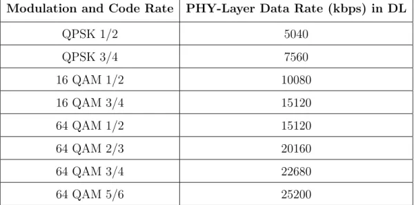
Modulation and Code Rate PHY-Layer Data Rate (kbps) in DL

QPSK 1/2 5040 QPSK 3/4 7560 16 QAM 1/2 10080 16 QAM 3/4 15120 64 QAM 1/2 15120 64 QAM 2/3 20160 64 QAM 3/4 22680 64 QAM 5/6 25200

Table 2.3: PHY layer data rate at channel bandwidths 10 MHz

The rates shown in Table 2.3 are the PHY layer data rate that is shared among all users given by Agilent web site [17]. The calculations here assume a frame size of 5 ms, a 12.5 percent OFDM guard interval overhead, and a PUSC subcarrier permutation scheme.

2.3

Scheduling

The aim of scheduling is to distribute the data regions (subcarriers) among the MSs based on QoS requirements and channel conditions. IEEE 802.16e [2] standard does not include a specific scheduling algorithm. In the simulations, we will use proportional fair (PF) scheduling.

2.3.1

Proportional Fair (PF) Scheduling

PF algorithm tries to maximize total network throughput and keep a minimal level of service for each user. PF algorithm schedules the user whose ratio of instantaneous achievable rate to average rate is maximum. In [5], the PF algorithm is described for OFDMA systems. Scheduled user, u∗, on the pth RB is determined as

u∗ = arg max_{u:1≤u≤Nsec}Ru,p[t] ru

(2.1)

where Nsec is the number of MSs per sector, t is the scheduling instant. The meaning of

a RB is the same with burst or data region that are explained in Section 2.1.2. Ru,p[t] is

the instantaneous achievable rate of user u on the pth _{RB at time t and is the function of}

a CQI feedback, which can be expressed as

Ru,p[t] = log2(CQIu,p[t]) (2.2)

where CQIu,r is the CQI sent by the uth MS for the rth RB. In Eq. 2.1, ru is the moving

average of the instantaneous rates of user u. Metric ru is updated after scheduling each

RB. The update is as follows,

ru =      αRu,p[t] + (1 − α)ru, u = u∗ (1 − α)ru, u 6= u∗ (2.3)

= Tf rame

P ×TP F where Tf rame is the duration of a WiMAX frame, P is the number of RBs and

TP F is the latency time.

In the simulations, scheduling is done at the beginning of each frame. The packets that need to be retransmitted are allocated to RBs with first priority.

2.3.2

Fairness

In WiMAX, while we try to maximize total wireless network throughput, we are also interested in the distribution of the total network throughput among MSs. In traditional frequency reuse techniques (i.e, 1x3x3, 3x3x1), MSs that are close to cell edge experience unacceptable level of interference since they are distant to corresponding BS and this causes low throughput for these users. Since each MS in a cell should have a good quality of service, we need to make sure that the throughput of each MS should be similar to each other. For this purpose, we use Jain’s fairness index [18] which measures how the total cell throughput is distributed among users. Jain’s fairness index is defined as

f (x1, x2, ..., xn) = (Pn i=1 xi)2 nPn i=1 (xi)2 (2.3)

where n is the number of total users, xi is the throughput for i’th connection. The fairness

index always lies between 0 and 1. Jain’s fairness index achieves the maximum value of f = 1 when xi = constant for all i.

In this chapter, we introduce some important concepts in WiMAX. In next chapter, we introduce the wireless channel model, frequency reuse models and fractional frequency reuse concept with the system level simulation methodology.

Chapter 3

System Level Simulation of WiMAX

3.1

Frequency Reuse Models

Since we are given a certain number of channels in a frequency band, in order to serve certain amount of users and to have a good coverage area, we need to use the channels efficiently. In the case of a BS is to provide service over a wide area, it must have high power and have a good location (possibly highest location) available in the coverage area. However, if the BS transmits with high power, the channel allocated to transmit site can not be reused for a considerable distance and then capacity is limited. This leads to the frequency reuse concept which limits the power of BS and use frequency repeatedly in the same area.

Frequency reuse is a technique which requires the partitioning of a cell into segments of a cell which are called sectors. In frequency reuse, we allocate the same spectrum band to different sector or cells. A frequency reuse model is denoted by a triple Nc x Ns x Nf

[19], where Nc is the number of cells in the network cluster. It determines the inter-cellular

frequency reuse. Ns represents the number of sectors in a cell and Nf demonstrates

intra-cellular frequency reuse. In other words Nc is the ratio of the entire bandwidth to the

bandwidth allocated for each cell, Ns is the number of sectors per cell and Nf is the ratio of

the bandwidth allocated for a cell to the bandwidth allocated for a sector. Two frequency reuse patterns 1x3x3 and 3x3x1 are illustrated in Figure 3.1. In 1x3x3 reuse mode, each cell in the network is assigned whole spectrum but the whole spectrum is divided into

three segments, namely f1, f2, and f3, and each sector in a particular cell is assigned only one of the segments. In 3x3x1 reuse mode, the whole spectrum band is divided into three segments, namely f1, f2, and f3 and each cell is assigned only one of the segments. Sectors in a particular cell are assigned the same segment.

In this thesis, we consider the deployment of WiMAX as a cellular network. Each cell in the network has a hexagonal structure and has a single BS in the center. A cell is divided into a number of sectors (typically 3) in order to increase frequency reuse by reducing interference to other cells and sectors. A directional antenna is placed at the BS for each sector in the cell.

Figure 3.1: Frequency reuse patterns

3.1.1

Fractional Frequency Reuse

Fractional frequency reuse (FFR) is a technique which divides the cell into two distinct regions: the inner cell and outer cell. MSs in the inner cell can use the entire frequency band, while MSs in the outer cell use a fraction of the frequency band. Transmission in the inner and outer cells occur during different time periods so that users at the cell edge experience less interference.

Figure 3.2 shows the network deployment for the FFR model that will be studied in this thesis. In FFR, each cell in the network is assigned whole spectrum but for the outer cell, whole spectrum is divided into three segments, namely f1, f2, and f3, and each sector in outer cell is assigned only one of the segments. MS inside the inner cell use the entire frequency band (F).

Figure 3.2: Illustration of FFR

In conventional cellular planning methods; MSs that are close to cell edge, experience unacceptable level of interference since they are distant to corresponding BS and this causes low throughput for these users. In FFR method, cell edge users can get special treatment (by allocating more resource) to bring better signal quality for cell edge users. FFR maxi-mizes spectral efficiency for users at the inner cell (with full frequency reuse) and improves signal quality and throughput for users at a cell edge.

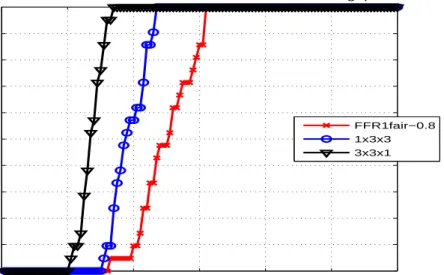
For a better understanding that why we can use FFR technique instead of using tradi-tional frequency reuse models (i.e, 1x3x3, 3x3x1), the throughput distributions of the three frequency reuse methods are compared in Figure 3.3.

In Figure 3.3, the radius of the inner cell is 0.8 km. From Figure 3.3, we observe that with 90% sector throughput is 6.2 MBit/s for FFR, is 4.3 MBit/s for 1x3x3 and is 3 MBit/s for 3x3x1. FFR provides much better results than 1x3x3 and 3x3x1.

In [8], there are two regions as inner and outer cells. In the inner cell the whole frequency band is used. In the outer cell, whole spectrum is divided into three segments, namely f1, f2, and f3 and each cell uses one of the segment. An illustration of the FFR used in [8] can be seen in Figure 3.4. The FFR used in this thesis requires sectoring in the outer cell. Whole spectrum is divided into three segments, namely f1, f2, and f3, and each sector in outer cell is assigned only one of the segments. By using sectoring in the outer cell, cell edge users experience less interference since the adjacent sectors use different frequency

0 2 4 6 8 10 12 0 0.1 0.2 0.3 0.4 0.5 0.6 0.7 0.8 0.9 1

Cumulative Distribution Function of Sector Throughput

Sector throughput (Mbit/s)

P[Sector throughput < abscissa]

FFR1fair−0.8 1x3x3 3x3x1

Figure 3.3: CDF of section throughput

segments.

Figure 3.4: Illustration of FFR used in [8]

In [9] and in [10], used FFR model is the same with the model we use in this thesis. Main objective in [9] is to maximize the overall network utility. In [10], total power within each sector is upper bounded and main concentration is on power usage of each user. In this thesis, we concentrate on the cell throughput and the distribution of the throughput among MS.

In the next chapter, we will discuss how to adjust the parameters of FFR in order to get higher throughput for cell edge users while having maximum spectral efficiency for inner cell users.

3.2

Simulation Methodology

In this section, we will introduce the parts of the system level simulation which are con-figuration, initialization, simulation, and analysis. OFDMA parameters and systems pa-rameters that are the same in each simulation scenario are given in Table 3.1 and Table 3.2.

Parameter Value

Bandwidth 10 MHz

Sampling frequency 11.2 MHz

FFT size 1024

Ratio of DL subframe duration to frame duration 1/2

Subcarrier spacing 10.94 kHz

OFDMA symbol duration 102.86 µs

Null subcarriers 184

Pilot subcarriers 120

Data subcarriers 720

Frame duration 5 ms

Number of OFDM symbols in frame 48

Number of OFDM symbols in DL subframe 29

Number of OFDM symbols allocated to preamble, 5

DL-MAP and UL-MAP messages

Number of OFDM symbols allocated to DL data regions 24 Number of data subcarriers allocated to subchannel 24

Slot size 1 subchannel x 2 OFDM symbol

Parameter Value

Number of clusters 1

Number of cells per cluster 7

Number of sectors per cell 3

Number of sectors per cluster 21

Carrier Frequency 2.5 GHz

BS to BS distance 1.5 km

Minimum MS to BS distance 35 m

MS noise figure 7 dB

BS transmit power per sector/subcarrier 46 dBm De-correlation distance for shadowing 50 m Log normal shadowing standard deviation 8 dB

CQI feedback delay 3 frames

Maximum number of HARQ retransmissons 3 frames Minimum HARQ retransmisson delay 2 frames

Number of strong interferers 8

Table 3.2: System level simulator parameters

3.2.1

Configuration

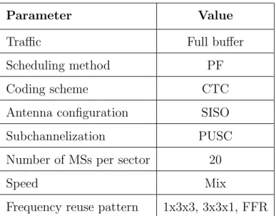
In the configuration part, a simulation scenario is determined by the parameters given in Table 3.3. Speed input is “mix”: %60 of MSs have 3 km/h speed, %30 of MSs have 30 km/h speed, and %10 of MSs have 120 km/h speed.

In Single-Input and Single-Output (SISO), there is only one antenna both in the trans-mitter and receiver. In addition to the parameters given in Table 3.3, simulation time is also specified in the configuration phase. Simulation time, Tsim, indicates the duration of

Parameter Value

Traffic Full buffer

Scheduling method PF

Coding scheme CTC

Antenna configuration SISO

Subchannelization PUSC

Number of MSs per sector 20

Speed Mix

Frequency reuse pattern 1x3x3, 3x3x1, FFR Table 3.3: Input parameters

3.2.2

Initialization

In the initialization part, the cellular structure is generated. The cellular structure used in this thesis is given in Figure 3.5 where there is 1 cluster that includes 7 cells and each cell has 3 sectors.

Figure 3.5: Cellular deployment

Subcarriers are distributed to the sectors according to the frequency reuse pattern. As-signed subcarriers to the sectors are permuted with the selected subchannelization scheme, Partially Used Sub-Carrier (PUSC). WiMAX uses the same OFDMA subchannelization structure and its extension to address mobility has retained the OFDMA concept for Fully Used Subcarrier (FUSC) and PUSC. Use of FUSC, mainly in the DL, and PUSC in both

DL and UL.

3.3

Simulation Procedure and Flow

• MSs are randomly and independently placed to the each cluster. Placing stops when the number of MSs that each sector serves reaches to 20.

• We assume MSs do not move during the placement so they remain attached to the same BS.

• The speed of each MS is determined such that %60 of MSs have 3km/h speed, %30 of MSs have 30 km/h speed, and %10 of MSs have 120 km/h speed. The assigned speeds are used only to model the Doppler effect.

• In the simulations, we make scheduling at the beginning of each frame. The packets that need to be retransmitted are allocated to RBs with first priority.

• We assume queue sizes are infinite so that packets are not blocked when they come into the system.

• CQI is reported for each RB. Packets are retransmitted as necessary.

More information about the system level simulator can be found at [5] and [20].

3.3.1

Metric Computation

At the end of each placement, we calculate the performance metrics for each MS and sector on the cluster and store them to use at the “Analysis” part. Performance metrics are user data throughput, sector data throughput, user average packet retransmission, and spectral efficiency. Descriptions of these metrics are as follows.

User data throughput is the ratio of the number of successfully received information bits to the simulation time for the MS of interest. User data throughput is computed as:

T(u) = N_packet(u) P p=1 Bu,p (bps) (3.1)

where T(u) _{is the data throughput of MS u, N}(u)

packet is the number of successfully received

packets for the uth_{MS, B}

u,pis the number of information bits at the pthsuccessfully received

packet for the uth _{MS, and T}

sim is the simulation time.

Sector data throughput is the sum of the data throughput of the MSs that are served by the sector of interest and computed as:

S(s)=

Nsec

X

i=1

T(ui) _{(bps) (3.2)}

where S(s) is the data throughput for the sth sector and (u1,u2,...,uNth) are the indexes of

the MSs served by sector s.

Spectral efficiency is computed once the sector throughputs of each sector are com-puted. Spectral efficiency is computed as:

SE = S

BW × T D (3.3)

where S is the average sector throughput, BW is the bandwidth assigned to each sector and TD is the ratio of the DL subframe duration to the frame duration.

User average packet retransmission is the average retransmission of the packets successfully received by the MS of interest and computed as:

T(u) = N_packet(u) P p=1 ru,p N_packet(u) (bps) (3.4)

where T(u) is the average packet retransmission for MS u and ru,p is the number of the

retransmission of the pth _{successfully received packet for the u}th _MS.

MS and the distance of MSs to their serving sectors are stored.

3.3.2

Analysis

In the analysis part, performance metrics that we store at each drop are loaded and com-bined. We have performance information of Muser, MSs and Msector sectors where

Muser = Ndrop× C × Nsec (3.5)

Msector = Ndrop× C (3.6)

and C is the number of sectors per cluster as given in Table 3.2. Based on these information, cumulative distributions of the user average throughput sector throughput, and user average packet retransmission are plotted. Figures including the distribution of MCSs are also plotted.

We have used a WiMAX system level simulator in MATLAB based on EMD document. We consider the deployment of WiMAX as a cellular network. Each cell in the network has a hexagonal structure and has a single BS in the center. A cell is divided into 3 sectors in traditional frequency reuse patterns and 4 sectors in FFR as can be seen in Figures 1.2 and Figure 1.3, in order to increase frequency reuse by reducing interference to other cells and sectors. A directional antenna is placed at the BS for each sector in the cell. Then we analyze system level performance of frequency reuse patterns.

In the simulator, we implement FFR in both statically and adaptively. In static FFR, before the simulation starts, we assign subchannels to users with respect to sector areas and with respect to user distribution under mobility, and use same subchannel allocation for the duration of simulation. In adaptive FFR, we start with the optimum fixed subcarrier allocation and we adjust the ratio of subcarriers allocated for the inner cell over time. In next section we talk about the performance evaluation of static and adaptive FFR.

Chapter 4

Performance Evaluation of Static and

Adaptive FFR

In this chapter, we first introduce static FFR and adaptive FFR concepts. Then we provide user data throughput, sector data throughput, user average packet retransmission and burst profile histograms for the performance metrics. At the end of the chapter, we make some comparison of static and adaptive FFR, and then we show that by dynamically adjusting the ratio of subcarriers allocated to the inner cell based on the user distribution, the throughput-fairness index product can be increased by about 5% compared with the fixed optimum subcarrier allocation.

In the simulations, simulation time is 1.5 seconds. We analyze 300 frames. Default values, given in Table 4.1, are used for the input parameters unless otherwise stated.

Parameter Value

Traffic Full buffer

Scheduling method PF

Coding scheme CTC

Antenna configuration SISO

Subchannelization PUSC

Number of MSs per sector 10

Speed Mix

Frequency reuse pattern 1x3x3, 3x3x1, FFR Table 4.1: Default input parameters

In 1x3x3 and 3x3x1, we divide the cell into 3 sectors but in FFR case we divide the cell into 4 sectors as shown in Figure 4.1 and Figure 4.2 in order to increase frequency reuse

by reducing interference to other cells and sectors. A directional antenna is placed at the BS for each sector in the cell.

Figure 4.1: Frequency reuse patterns

Figure 4.2: Illustration of the FFR

In Figure 4.3, we can see the DL subframe for FFR scheme. In this figure; F zone is the sum of all subchannels available and is used by inner cell users, f1, f2 and f3 zones are fractions of all subchannels available and is used by the outer cell sectors. Since we use 120◦ sectoring in FFR, f1, f2 and f3 are equal to each other. When we increase the F zone, we have much better throughput performance for the inner cell users but in return there is not enough subcarriers for users that are in outer cell sectors so the fairness index becomes worse.

One of the key factors determining the FFR performance is how to assign subcarriers to users in order to get higher throughput and fairness index. We assign the subcarriers

Figure 4.3: DL subframe for FFR scheme

to the users both statically and adaptively. In static FFR, as shown in Figure 4.3, we fix frequency reuse zones (F, f1, f2 and f3) and allocate subcarriers to each user from the subset of subcarriers assigned to the zone corresponding to the location of the MS. In adaptive FFR, we start with the optimum fixed subcarrier allocation and we adjust the ratio of subcarriers allocated for the inner cell over time. In Figure 4.4, in simulation period 1 we start with optimum fixed subcarrier allocation but in simulation period 2, we changed the allocation and increase the duration of F zone where t1 > t0 in order to increase the multiplication of total cell throughput and fairness index.

4.1

Static FFR

In static FFR, before the simulation starts, we assign subchannels to users with respect to sector areas and with respect to user distribution under mobility, and use same subchannel allocation for the duration of simulation.

4.1.1

Subchannel Allocation with Respect to Sector Areas

In subchannel allocation with respect to sector areas, we assign subchannels to inner and outer areas in proportion with the area of regions. We assume that there is a under uniform distribution of users, thus the number of users in a cell is proportional to the square of the radius of the cell. If there are n users in a cell with radius r, we expect there are 4n users in a cell with radius R=2r. ( In the annulus shape (shown in Figure 4.5), there are 3n users.) In our simulations, BS to BS distance is 1.5 km. So outer radius is found with the equation:

R = BStoBSdistance

2 × Cos(π/6) (4.1)

and R is calculated as 0.866 km.

For inner radius (r) we have 3 different scenarios: r=0.4R, r=0.6R and r=0.8R. In this section, we assign subchannels to inner and outer areas such that subchannels are allocated in proportion with the area of the region.

For r=0.4R we allocate 16% of total subchannels into inner cell, for r=0.6R we allocate 36% of total subchannels into inner cell and for r=0.8R we allocate 64% of total subchannels into inner cell and remaining subchannels are assigned to outer cell sectors evenly. For the rest of the thesis, for simplicity we assume that R=1.

Figure 4.6 displays the user throughput distribution of the reuse patterns. We observe that the throughput performance of FFR pattern with inner radius r=0.8 is better than the other reuse patterns’ throughput performance. The reason is as follows. In 1x3x3 and 3x3x1 reuse patterns, each sector is assigned one third of the entire bandwidth. But in

Inner radius (r) Inner cell resource percentage

0.4 16

0.6 36

0.8 64

Table 4.2: Percentage of inner cell users to all users for different inner radiuses

Figure 4.5: Circular figure

FFR cases, the inner sector is assigned the entire bandwidth so the overall performance is better than traditional reuse patterns. Among the FFR patterns, with inner radius r=0.8 is best. That is because of in that pattern, we have assigned a large portion, 64% of all subchannels for the inner sector where users that can achieve higher throughputs.

Figure 4.7 displays the sector throughput of the reuse patterns. We observe that the throughput performance of FFR pattern with inner radius r=0.8 is better than the other reuse patterns’ throughput performance. The reason is the same with the user throughput case.

0 500 1000 1500 0 0.1 0.2 0.3 0.4 0.5 0.6 0.7 0.8 0.9 1

Cumulative Distribution Function of User Throughput

User throughput (kbit/s)

P[User throughput < abscissa]

FFRstatic1−0.4 FFRstatic1−0.6 FFRstatic1−0.8 1x3x3

3x3x1

Figure 4.6: CDF of user throughput

0 2 4 6 8 10 12 0 0.1 0.2 0.3 0.4 0.5 0.6 0.7 0.8 0.9 1

Cumulative Distribution Function of Sector Throughput

Sector throughput (Mbit/s)

P[Sector throughput < abscissa]

FFRstatic1−0.4 FFRstatic1−0.6 FFRstatic1−0.8 1x3x3

3x3x1

Figure 4.7: CDF of sector throughput

Figure 4.8 displays the average user throughput as a function of the distance for the reuse patterns. We observe that the average throughput performance of 3x3x1 is worst. In 3x3x1, all sectors in a cell are using same subchannels so interference is high and it makes throughput worse even for MSs close to the BS. 1x3x3 frequency reuse pattern provide good throughput results for MSs close to the BS. But when the distance of MS and BS increases,

0 200 400 600 800 1000 0.05 0.1 0.15 0.2 0.25 0.3 0.35 0.4 0.45

Distance from serving base station (meters)

Average user throughput (Mbit/s)

Average user throughput vs distance

FFRstatic1−0.4 FFRstatic1−0.6 FFRstatic1−0.8 1x3x3

3x3x1

Figure 4.8: Average user throughput vs. distance

throughput performance of 1x3x3 dramatically decreases and for the cell edge users, the throughput decreases under the value of 0.1 Mbit/s. In FFR patterns, we see some increases when distance from base station increases. We observe that with FFR, users at the outer sectors may achieve higher throughputs than the users in the inner sector since users within the outer sectors are allocated some dedicated subchannels. On the other hand, users away from the BS achieve significantly lower throughputs when 1x3x3 and 3x3x1 reuse patterns are used.

Table 2.3 gives us corresponding data rate in DL when different modulation and code rates are used, and we can see that with CTC-64QAM 5/6, PHY-layer data rate is 25200 kbps (the fastest) and with CTC-QPSK 1/2, PHY-layer data rate is 5040 kbps (the slowest) in DL.

Now we investigate percentage of selected MCSs. Figures 4.9, 4.10, 4.11 display per-centage of MCS selection for FFR with r=0.4, r=0.6 and r=0.8, respectively. Figure 4.12 and Figure 4.13 display percentage of MCS selection for 1x3x3 and 3x3x1, respectively. Since CTC-64QAM 5/6 makes the fastest data rate in DL, users that use CTC-64QAM 5/6 with higher percentage have higher throughput values. For example in Figure 4.8, for users that are 100 meters distant to BS, 1x3x3 has the best throughput performance since

in burst profile histogram users that are 100 meters distant to BS use CTC-64QAM 5/6 with 100% as can be seen in Figure 4.12. In Figure 4.9, we observe a sudden increase of CTC-64QAM 5/6 around 400 meters from BS which is the boundary between inner and outer sectors. We observe similar increase around 600 meters in Figure 4.10 and around 800 meters in Figure 4.11. This increases cause average user throughput increase in Figure 4.8. Normally when the distance increases, we expect average user throughput decreases. Because of CTC-64QAM 5/6 profile increases when the boundary between inner and outer sectors is traversed, users that are in the outer sectors can communicate at higher speeds and average user throughput increases in Figure 4.8. We have minimum fairness index performance from 1x3x3 frequency reuse pattern since from Figure 4.12, the users that are close to BS communicate at high speeds and they have high throughput values but the users that are in the cell edge can communicate at lowest speeds and they have really low throughput values so fairness index is minimum for 1x3x3 frequency reuse pattern and have the value of 0.27. Fairness index performance of 3x3x1 is better than 1x3x3 since there is not much difference of throughput value between the MSs that are close to BS and MSs that are in the cell edge as can be seen in Figure 4.13. Actually we have best fairness index performance with the value of 0.8608 in 3x3x1 frequency reuse pattern. We can see that throughput values of MS in 3x3x1 frequency reuse pattern do not change as much as in the other frequency reuse patterns from Figure 4.8 so best fairness index performance belongs to 3x3x1 frequency reuse pattern.

0 200 400 600 800 1000 0 0.1 0.2 0.3 0.4 0.5 0.6 0.7 0.8 0.9 1 FFR1fair−0.4

Distance from serving BS (meters)

Percentage of MCS selecton CTC−QPSK 1/2 CTC−QPSK 3/4 CTC−16QAM 1/2 CTC−16QAM 3/4 CTC−64QAM 1/2 CTC−64QAM 2/3 CTC−64QAM 3/4 CTC−64QAM 5/6

Figure 4.9: Burst profile histograms for FFR with r=0.4

0 200 400 600 800 1000 0 0.1 0.2 0.3 0.4 0.5 0.6 0.7 0.8 0.9 1 FFR1fair−0.6

Distance from serving BS (meters)

Percentage of MCS selecton CTC−QPSK 1/2 CTC−QPSK 3/4 CTC−16QAM 1/2 CTC−16QAM 3/4 CTC−64QAM 1/2 CTC−64QAM 2/3 CTC−64QAM 3/4 CTC−64QAM 5/6

Figure 4.10: Burst profile histograms for FFR with r=0.6

Figure 4.14 displays the cdf of users average number of packet retransmissions for the reuse patterns. We observe that the performance of 1x3x3 is the best one and the perfor-mance of the FFR with inner radius 0.8 is the worst one. This result is expected because the throughput is largest in FFR with inner radius 0.8 and therefore with high probability we will need more retransmissions. But because of the throughput is smallest in 1x3x3, we will need less retransmissions. This phenomenon is also called “Highest throughput, highest retransmission probability”. [21]

0 200 400 600 800 1000 0 0.1 0.2 0.3 0.4 0.5 0.6 0.7 0.8 0.9 1 FFR1fair−0.8

Distance from serving BS (meters)

Percentage of MCS selecton CTC−QPSK 1/2 CTC−QPSK 3/4 CTC−16QAM 1/2 CTC−16QAM 3/4 CTC−64QAM 1/2 CTC−64QAM 2/3 CTC−64QAM 3/4 CTC−64QAM 5/6

Figure 4.11: Burst profile histograms for FFR with r=0.8

0 200 400 600 800 1000 0 0.1 0.2 0.3 0.4 0.5 0.6 0.7 0.8 0.9 1 1x3x3

Distance from serving BS (meters)

Percentage of MCS selecton CTC−QPSK 1/2 CTC−QPSK 3/4 CTC−16QAM 1/2 CTC−16QAM 3/4 CTC−64QAM 1/2 CTC−64QAM 2/3 CTC−64QAM 3/4 CTC−64QAM 5/6

Figure 4.12: Burst profile histograms for 1x3x3

4.1.2

Subchannel Allocation with Respect to User Distribution

Under Mobility

We now discuss static FFR when the subchannels are allocated based on the expected number of users within the sectors. In order to calculate the distribution of users, we use

0 200 400 600 800 1000 0 0.1 0.2 0.3 0.4 0.5 0.6 0.7 0.8 0.9 1 3x3x1

Distance from serving BS (meters)

Percentage of MCS selecton CTC−QPSK 1/2 CTC−QPSK 3/4 CTC−16QAM 1/2 CTC−16QAM 3/4 CTC−64QAM 1/2 CTC−64QAM 2/3 CTC−64QAM 3/4 CTC−64QAM 5/6

Figure 4.13: Burst profile histograms for 3x3x1

0 0.5 1 1.5 2 2.5 3 0 0.1 0.2 0.3 0.4 0.5 0.6 0.7 0.8 0.9 1

CDF of user average packet retransmission

User average packet retransmission

P[User average packet retransmission < abscissa]

FFRstatic1−0.4 FFRstatic1−0.6 FFRstatic1−0.8 1x3x3

3x3x1

Figure 4.14: CDF of user average packet retransmission

a mobility model.

The Random Waypoint (RWP) mobility model for evaluating the performance of ad hoc routing protocols was first proposed in [22] (however, the name RWP was introduced later in [23]). The following description of RWP is taken from [11].

MS, and how their location, velocity and acceleration change over time [11]. RWP process represents the movement of a node within a convex area A ⊂ R2 _{and can be described}

as follows. Initially, the node is placed at a random point P1 chosen from a uniform

distribution over convex area A. Then a destination point P2 is randomly chosen from a

uniform distribution over A and the node moves along a straight line from P1 to P2 with

constant velocity V1 drawn with pdf fV(v). When the node reaches P2, a new destination

point, P3, is drawn independently from a uniform distribution over A and velocity V2 is

drawn from fV(v). The node again moves at constant velocity V2 to the point P3, and the

process repeats. This is illustrated in Figure 4.15.

Figure 4.15: RWP model illustrated

The radial distribution of mobile users in the RWP model are calculated in [11]. We use this in order to calculate the average ratio of users in the inner cell which is given in Table 4.3.

Inner radius (r) Percentage of inner cell users to all users

0.4 40

0.6 64

0.8 91

Table 4.3: Percentage of inner cell users to all users for different inner radiuses

Figure 4.16 displays the user throughput of the reuse patterns. We observe that the throughput performance of FFR pattern with inner radius r=0.8 is better than the other

0 500 1000 1500 0 0.1 0.2 0.3 0.4 0.5 0.6 0.7 0.8 0.9 1

Cumulative Distribution Function of User Throughput

User throughput (kbit/s)

P[User throughput < abscissa]

FFRstatic2−0.4 FFRstatic2−0.6 FFRstatic2−0.8 1x3x3

3x3x1

Figure 4.16: CDF of user throughput for RWP

reuse patterns’ throughput performance similar to the case where subchannels are allo-cated with respect to sector areas as discussed in Section 4.1.1. We also observe that user throughputs are higher when the subchannels are allocated based on average user density compared with allocation based on areas. That is because we assign much subchannels to the inner sector when subchannels are allocated based on user density as it can be observed from Table 4.3.

Figure 4.17 displays the sector throughput of the reuse patterns. We observe that the throughput performance of FFR pattern with inner radius r=0.8 is better than the other reuse patterns’ throughput performance. Actually we have better results in terms of sector throughput in every frequency reuse scheme with respect Section 4.1.1. So by using subchannel allocation with respect to user distribution under mobility we have better results than using subchannel allocation with respect to sector areas.

Figure 4.18 displays the average user throughput vs distance of the reuse patterns. Different from Figure 4.8, we observe no sharp increases in FFR user throughputs when the boundary between inner and outer sectors is traversed. That is because, we assign more subchannels to the inner sector, for the outer sectors there is not much subchannel left so

0 2 4 6 8 10 12 0 0.1 0.2 0.3 0.4 0.5 0.6 0.7 0.8 0.9 1

Cumulative Distribution Function of Sector Throughput

Sector throughput (Mbit/s)

P[Sector throughput < abscissa]

FFRstatic2−0.4 FFRstatic2−0.6 FFRstatic2−0.8 1x3x3

3x3x1

Figure 4.17: CDF of sector throughput for RWP

0 200 400 600 800 1000 0 0.1 0.2 0.3 0.4 0.5 0.6 0.7

Distance from serving base station (meters)

Average user throughput (Mbit/s)

Average user throughput vs distance

FFRstatic2−0.4 FFRstatic2−0.6 FFRstatic2−0.8 1x3x3

3x3x1

Figure 4.18: Average user throughput vs. distance for rwp

4.1.3

Throughput vs. Fairness

Until now, we have examined the average throughput performance for frequency reuse patterns. Now we will discuss the distribution of the total throughput among users.

In a communication system, it may be tempting to optimize the spectrum efficiency (i.e. the throughput). However, that might result in scheduling starvation of “expensive” users at far distance from the access point, whenever another active user is closer to the same or an adjacent BS. Thus the users would experience unstable service, perhaps resulting in a reduced number of happy customers. We try to optimize fairness and achieving high spectral efficiency. For this purpose, we use Jain’s fairness index which measures how the throughput is shared among users. Fairness index is 1 if the throughput of each connection is same. We try to maximize the fairness index while achieving high throughput.

0 10 20 30 40 50 60 70 0 0.1 0.2 0.3 0.4 0.5 0.6 0.7 0.8 0.9 1

Weighted Throughput vs Fairness Index for inner radius 0.6

Inner cell resource percentage

Weighted throughput Fairness index Inner throughput

Figure 4.19: Weighted throughput vs. fairness index

We have user throughput for all 420 users in the network and we want to talk about the total throughput of the network. We know the distance of each MS to BS and group them in distance intervals to BS (0-100 meters, 100-200 meters, ..., 900-1000 meters). We multiply throughput of each MS with the total number of MS in the same distance interval, then sum them up and finally divide by 420. We define this number as weighted throughput. Inner throughput is the sum of the throughput for the inner cell users.

In Figure 4.19, we can see the comparison of weighted throughput and fairness index for the inner cell radius r=0.6. For the inner cell users, we have assigned 10% to 64% of the whole subchannels. When we assign more subchannels to the inner cell users, we see decrease in fairness index while we see increase in throughput. Actually this is an expected result. Because for a fair system, we need to assign more resources to the outer cell users since their distance to BS is large and it causes to have less subchannels for inner cell users which can communicate at high speeds easily. If we give less resources to the outer cell users, the inner cell users which are much closer to the BS can communicate at higher speeds and to have better throughput performances but it results in an uneven distribution of throughput for inner cell and outer cell users and it reduces the fairness index.

Now we define a new term ρ as:

ρ = #ofinnercellusers

totalnumberofusers (4.2)

ρ represents the inner cell user percentage. For 3 values of ρ, we have compared the weighted throughput and fairness index.

For ρ = 0.1, we have assigned 10% of the whole users, 42, to the inner cell and the remaining 378 users to the outer cell.

For ρ = 0.4, we have assigned 40% of the whole users, 168, to the inner cell and the remaining 252 users to the outer cell.

For ρ = 0.7, we have assigned 70% of the whole users, 294, to the inner cell and the remaining 126 users to the outer cell.

The weighted throughput is plotted in Figure 4.20 as a function of the ratio of subchan-nels allocated for the inner cell for different values of ρ. In Figure 4.20, we can observe that for any value of ρ, the throughput increases when we increase the inner cell resource percentage. Actually we expect this result, because if we assign much resources for the inner cell users which are closer to the BS they can communicate at higher speeds and this increases the total throughput of the system. Also from the Figure 4.20, we can see that when we assign less than 60 % of the whole resources to the inner cell users, the throughput is maximized for ρ = 0.4. When we assign more than 60% of the whole resources to the inner cell users, we have maximum throughput for ρ = 0.1.

0 20 40 60 80 100 0 0.1 0.2 0.3 0.4 0.5 0.6 0.7

Inner cell resource percentage

Weighted throughput

ρ = 0.1

ρ = 0.4

ρ = 0.7

Figure 4.20: Weighted throughput vs inner cell resource percentage for different ρ values

0 20 40 60 80 100 0 0.1 0.2 0.3 0.4 0.5 0.6 0.7 0.8 0.9 1

Inner cell resource percentage

Fairness Index

ρ = 0.1

ρ = 0.4

ρ = 0.7

Figure 4.21: Fairness index vs inner cell resource percentage for different ρ values

The fairness index is plotted in Figure 4.21 as a function of the ratio of subchannels allocated for the inner cell for different values of ρ. In Figure 4.21, we can observe that when we assign 10% of the whole resources to the inner cell users, the worst fairness performance is obtained from ρ = 0.7 and that is because we assign 10% of the whole resources to 70% of whole users and 90% of whole resources to the 30% of whole users. When the ratio

of subchannels allocated to inner cell exceeds 50%, we can see much better performance for ρ = 0.7 since we assign much resources for larger number of users. As we expect, the worst performance belongs to ρ = 0.1 for higher inner cell resource percentages since we try to assign more resources for small number of users and less resources for large amount of users.

When we increase the inner cell resource percentage, the throughput increases for any value of ρ as can be seen in Figure 4.20 and fairness index decreases for any value of ρ as can be seen in Figure 4.21. We need to have a balance between throughput and fairness index. With this purpose, we investigate the multiplication of throughput and fairness index. Throughput x fairness index is plotted in Figure 4.22 as a function of the ratio of subchannels allocated for the inner cell for different values of ρ.

0 20 40 60 80 100 0 0.05 0.1 0.15 0.2 0.25 0.3

Inner cell resource percentage

ρ = 0.1 fairness*throughput ρ = 0.4 fairness*throughput ρ = 0.7 fairness*throughput

Figure 4.22: Fairness index × throughput for different inner cell resource percentages

Before we process the adaptive FFR, we investigate multiplication of cell throughput and fairness index for traditional frequency reuse techniques and static FFR patterns. In Table 4.4, we can see the cell throughput, fairness index (F.I.) and the throughput fairness index product for the models we use in this thesis.

Frequency reuse pattern Throughput F.I. Throughput x F.I. 1x3x3 0,1899 0,2694 0,0513 3x3x1 0,0952 0,8608 0,0819 FFR wrt. sector areas r=0.4 0,1837 0,7533 0,1384 FFR wrt. sector areas r=0.6 0,2253 0,7688 0,1732 FFR wrt. sector areas r=0.8 0,2455 0,7546 0,1853 FFR wrt. RWP r=0.4 0,2608 0,7618 0,1987 FFR wrt. RWP r=0.6 0,2705 0,7534 0,2038 FFR wrt. RWP r=0.8 0,3101 0,6708 0,2080

Table 4.4: Throughput × fairness index for various frequency reuse patterns

4.2

Adaptive FFR

In static allocation, we observe that when the throughput of the network increases, the fairness index decreases. In order to combine these two performance metrics into a single metric, we use the throughput-fairness index product and study the trade-off between the two metrics. When the inner cell user percentage changes over time, we observe that by changing the ratio of subcarriers allocated for the inner cell, we can have better fairness × throughput performance. Since we adjust the ratio of subcarriers allocated for the inner cell over time, we call this method adaptive FFR.

In Figure 4.22, we observe that when the ratio of subchannels allocated for the inner cell is less than 65%, ρ=0.4 gives us better results than other ρ values and when the ratio of subchannells allocated for the inner cell is greater than 65%, ρ=0.7 gives us better results than other ρ values. So when ρ changes in time, we need to adjust the ratio of subchannels allocated for the inner cell changes in order to achieve best fairness × throughput performance. With this purpose, we propose adaptive FFR.

In Figure 4.22; we have seen that for ρ=0.7, we have best throughput x fairness in-dex performance at 90% inner cell resource percentage and for ρ=0.4, best throughput x fairness index performance at 50% inner cell resource percentage. After 65% of inner cell resource percentage, ρ=0.7 gives us best performance and before 65%, ρ=0.4 gives us best performance. So we decided to start with ρ=0.7 in first simulation and whenever ρ

value approaches to ρ=0.4, we will adjust the inner cell resource in order to achieve bet-ter throughput × fairness index performance. In Table 4.5, we can see the number and percentage of inner cell users when the frame number changes.

Frame Number Number of Inner Cell Users Percentage of Inner Cell Users

0 294 0.70

300 263 0.63

600 234 0.56

900 188 0.45

1200 169 0.40

Table 4.5: Frame number vs number of inner cell users

If we fix inner cell resource to 50% or 90% for all 5 simulations, we have following results.

Inner cell resource Throughput Fairness Index Throughput x Fairness Index

50% 0,3086 0,7008 0,2163

90% 0,4735 0,5048 0,2390

Table 4.6: Throughput × fairness index for fixed inner cell resources

In Figure 4.22; we have seen that for ρ=0.7, we have best throughput x fairness index performance at 90% inner cell resource percentage and for ρ=0.4, best throughput x fairness index performance at 50% inner cell resource percentage. So either by 50% or by 90% inner cell resource percentage, we have fixed optimum subcarrier allocation. Table 4.6 shows us by 90% allocation of resources to the inner cell, we have product of cell throughput and fairness index as 0.2390. So by 90% allocation of resources to the inner cell, we have fixed optimum subcarrier allocation.

For adaptive FFR, we check the percentage of inner cell users from Table 4.5, and assign 50% allocation of resources to the inner cell if the percentage of inner cell is less than 0.55, and assign 90% allocation of resources to the inner cell if the percentage of inner cell is greater than 0.55 in every simulation period (300 frames). The reason of choosing the value 0.55 is, it is the average of 0.4 and 0.7. We could make simulations for different values of ρ