Graph and hypergraph partitioning

ú i i í i t M β ί ΐ ΰ· i l l ¡ i l й &1ί lù t ft

G R A P H A N D H Y P E R G R A P H

PA R TITIO N IN G

A THESIS

SUBMITTED TO THE DEPARTMENT OF COMPUTER ENGINEERING AND INFORMATION SCIENCE AND THE INSTITUTE OF ENGINEERING AND SCIENCE

OF BILKENT UNIVERSITY

IN PARTIAL FULFILLMENT OF THE REQUIREMENTS FOR THE DEGREE OF

MASTER OF SCIENCE

tarcfindcn

By

All Da§dan

September, 1993

i

Tfc

II

I certify that I have read this thesis and that in my opinion it is fully adequate, in scope and in quality, as a thesis for the degree of Master of Science.

Cefoiet Aykai

Asst. Prof. Cefcfet Aykanat (Advisor)

I certify that I have read this thesis and that in my opinion it is fully adequate, in scope and in quality, as a thesis for the degree of Master of Science.

Asst. Prof. Kemal Oflazer

I certify that I have read this thesis and that in my opinion it is fully adequate, in scope and in quality, as a thesis for the d e g f^ of M a ^ r of Science.

■ n /

Approved for the Institute of Engineering and Science:

Prof. Mehmet Baray Director of the Institut

A BSTRA CT

GRAPH AND HYPERGRAPH PARTITIONING

All Da§dan

M.S. in Computer Engineering and Information Science

Advisor: Asst. Prof. Cevdet Aykanat

September, 1993

Graph and hypergraph partitioning have many important applications in var­ ious areas such as VLSI layout, mapping, and graph theory. For graph and hypergraph partitioning, there are very successful heuristics mainly based on Kernighan-Lin’s minimization technique. We propose two novel approaches for multiple-way graph and hypergraph partitioning. The proposed algorithms drastically outperform the best multiple-way partitioning algorithm both on randomly generated graph instances and on benchmark circuits. The proposed algorithms convey all the advantages of the algorithms based on Kernighan- Lin’s minimization technique such as their robustness. However, they do not convey many disadvantages of those algorithms such as their poor performance on sparse test cases. The proposed algorithms introduce very interesting ideas th at are also applicable to the existing algorithms without very much effort.

Keywords: Graph Partitioning, Hypergraph Partitioning, Circuit Partitioning,

Local Search Heuristics, Partitioning Algorithms

ÖZET

ÇİZGE VE HİPERÇİZGE PARÇALAMA

Ali Daşdan

Bilgisayar ve Enformatik Mühendisliği, Yüksek Lisans

Danışman: Yrd. Doç. Dr. Cevdet Aykanat

Eylül, 1993

Çizge ve hiperçizge parçalama, çok büyük ölçekli tümleşik devre tasarımı, paralel bilgisayarlarda hesaplama yükünün işlemcilere dağıtımı, çizge kuramı gibi bir çok alanda önemli uygulamaları olan işlemlerdir. Çizge ve hiperçizge parçalam a işlemleri için, Kernighan-Lin’in tekniğine dayanan çok başarılı buluşsal algoritmalar vardır. Biz bu çalışmamızda, çok yollu çizge ve hiperçizge parçalamak için iki tane yeni yaklaşım önerdik. Önerilen algoritmalar, rastgele üretilmiş çizge örneklerinde ve algoritmaları karşılaştırmak için kullanılan stan­ dart devrelerde şu anda çok yollu çizge ve hiperçizge parçalamak için kullanılan en iyi algoritmadan çok daha iyi sonuçlar verdi. Önerilen algoritmalar, eski algoritmaların çizge ve hiperçizge problemlerindeki yeni ve değişik gereklere kolayca uyarlanabilme gibi iyi özelliklerini taşımalarına rağmen, eski algorit­ m aların yoğunluğu çok seyrek olan çizge ve hiperçizge problemleri üzerinde kötü sonuçlar vermesi gibi kötü özelliklerini taşımamaktadırlar. Önerilen yaklaşımların getirdiği çok ilginç fikirler, eski algoritmalara da çok büyük bir çaba gerektirmeden uygulanabilir.

Anahtar Sözcükler: Çizge Parçalama, Hiperçizge Parçalama, Devre Parçalama,

Buluşsal Algoritmalar, Parçalama Algoritmaları

ACKNOWLEDGEMENTS

I would like to express my deep gratitude to my supervisor Dr. Cevdet Aykanat for his guidance, suggestions, and invaluable encouragement throughout the development of this thesis. I would like to thank Dr. Kemal Oflazer for his encouragement as well as for reading and commenting on the thesis. I would also like to thank Dr. Mustafa Akgul for reading and commenting on the thesis. I owe special thanks to Dr. Mehmet Baray for providing a pleasant environment for study. I am grateful to my family and my friends for their infinite moral support and help.

Bu çalışmamı,

herşeyimi borçlu olduğum anneme ve babama,

ve

ailemizin en küçük üyesi

Ceren’e

adıyorum.

C ontents

1 INTRODUCTION 1

1.1 Combinatorial Optimization P r o b le m s ... 1

1.2 Graph and Hypergraph Partitioning P ro b le m s... 2

1.3 Previous A p p ro ach es... 3

1.4 M otivation... 5 1.5 Experiments and R e su lts ... 7 1.6 O u tlin e... 7 2 GRAPH PARTITIONING 8 2.1 In tro d u ctio n ... 8 2.2 Basic C o n c e p ts ... 9 2.3 Graph Partitioning P ro b le m ... 11

2.4 Multiple-way Graph P a r titio n in g ... 13

2.4.1 Gain C o n c e p t... 13

2.4.2 Effects of a Vertex M o v e ... 14

2.4.3 Balance C o n d itio n s... 16

3 HYPERGRAPH PARTITIONING 18

3.1 In tro d u ctio n ... 18

3.2 Basic C o n c e p ts ... 18

3.3 Hypergraph Partitioning P ro b le m ... 22

3.4 Multiple-way Hypergraph P a r titio n in g ... 23

3.4.1 Gain C o n c e p t... 23 3.4.2 Effects of a Vertex M o v e ... 24 3.4.3 Balance C o n d itio n s... 29 4 PARTITIONING ALGORITHMS 31 4.1 Local S earch ... 31 4.2 Neighborhood S t r u c t u r e ... 35

4.3 Previous A p p ro ach es... 36

4.4 Bipartitioning versus Multiple-way P a r titio n in g ... 38

4.5 Data S tru c tu re s... 40

4.6 Reading Hypergraphs and G ra p h s ... 42

4.7 Initial Partitions ... 43

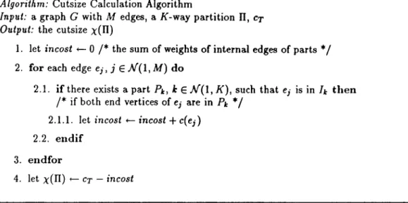
4.8 Cutsize C alcu latio n ... 45

4.9 Prefix Sum C alcu latio n ... 46

4.10 Main C l a i m ... 47

4.11 Partitioning by Locked M o v e s ... 49

4.12 Partitioning by Free M oves... 53

4.13 Complexity A n a ly s is ... 59

4.13.1 Time Complexity A n aly sis... 59

4.13.2 Space Complexity A nalysis... 61

5 EXPERIMENTS AND RESULTS 64 5.1 Implementation of A lg o rith m s... 64

5.2 Balance Condition ... 64

5.3 K-PFM A lg o rith m s... 65

5.4 K-PLM A lg o rith m s... 65

5.5 Comments on Neighborhood Structure of A lg o rith m s... 67

5.6 N o ta tio n ... 68 5.7 Test G r a p h s ... 69 5.7.1 Random Graphs ... 69 5.7.2 Geometric Graphs ... 69 5.7.3 Grid G ra p h s... 70 5.7.4 Ladder G r a p h s ... 71 5.7.5 Tree G ra p h s ... 71

5.8 Test H y p erg rap h s... 73

5.9 General Comments on E x p erim e n ts... 73

5.10 General Comments for Experiments on G rap h s... 74

5.11 Performance of K-PFM Algorithms on G r a p h s ... 74

5.11.1 Different Freedom Value F u n c tio n s ... 77

5.11.2 Determining Scale F a c to r... 78

5.12 Performance of K-PLM Algorithms on G r a p h s ...81

5.13 General Comments for Experiments on Hypergraphs ... 81

CONTENTS

5.14 Performance of K-PFM Algorithms on H ypergraphs... 82

5.15 Performance of K-PLM Algorithms on H ypergraphs... 83

5.16 Behaviour of Freedom Value F u n ctio n ... 84

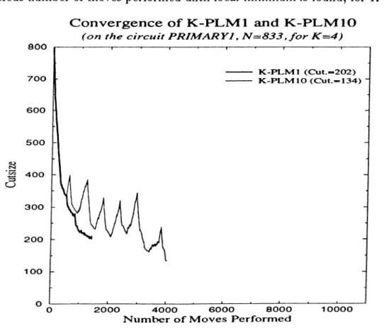
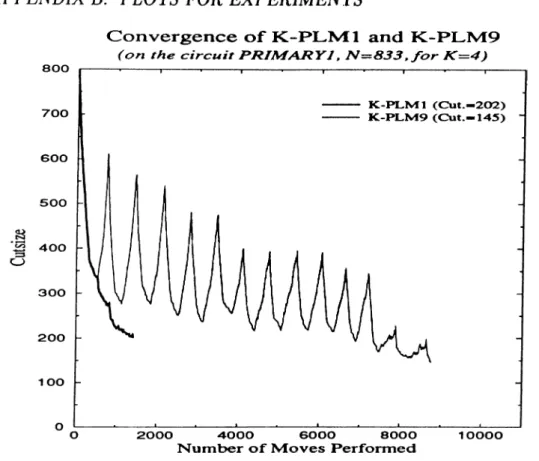
5.17 Convergence of A lgorithm s... 84

5.18 Distribution of Cutsizes ... 85

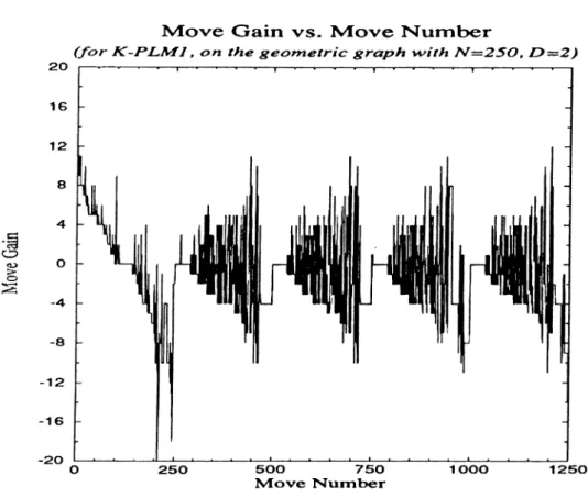
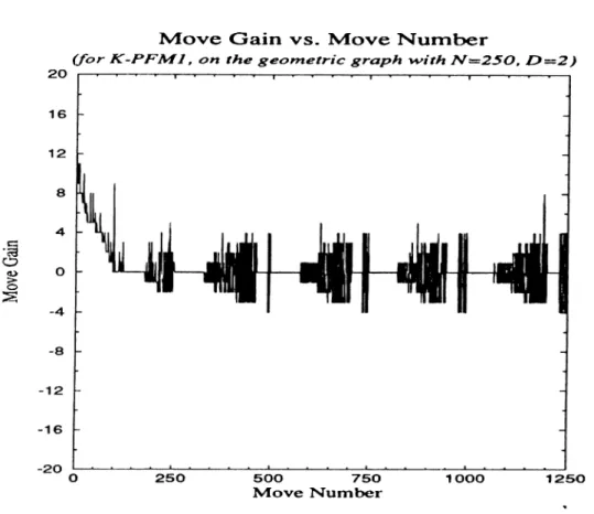
5.19 Distribution of Move Gains ... 86

6 CONCLUSIONS 87

7 APPENDICES 90

A FILE FORMATS 91

B PLOTS FOR EXPERIMENTS 93

List o f Figures

2.1 An algorithm for initial cost computation in a g ra p h ... 14

2.2 An algorithm for gain updates in a g r a p h ... 16

3.1 An algorithm for initial cost computation in a hypergraph . . . 25

3.2 An algorithm for gain updates in a hypergraph... 30

4.1 A general local search alg o rith m ... 34

4.2 Bucket data structure for a part in a given p a rtitio n ... 42

4.3 An initial partitioning algorithm ... 44

4.4 A cutsize calculation algorithm for graphs ... 45

4.5 A cutsize calculation algorithm for h y p e rg ra p h s ... 46

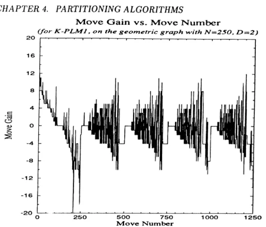
4.6 Change of gains of selected moves in Sanchis’ Algorithm (one pass contains 250 m o v e s)... 47

4.7 The generic direct multiple-way partitioning-by-locked-moves a lg o r i th m ... 50

4.8 The generic direct multiple-way partitioning-by-free-moves al­ gorithm ... 56

5.1 Random graph generation algorithm ... 70

5.2 Geometric graph generation algorithm ... 71

LIST OF FIGURES Xll

5.3 Grid generation a lg o r ith m ... 72

5.4 Tree generation a lg o r ith m ... 72

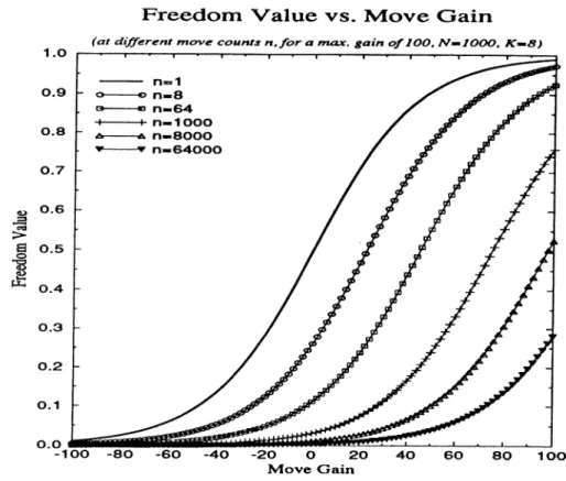
B.l Freedom Value for move gains at different move counts n, for

G,nax = 100, iV = 1000, and A' = 8 ... 94 B.2 Convergence of K-PLMl Algorithm, a plot of cutsize versus

number of moves performed until local minimum is found, for

К = 2,4, and 8 ... 94

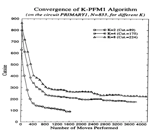
B.3 Convergence of K-PFMl Algorithm, a plot of cutsize versus number of moves performed until local minimum is found, for /F = 2,4, and 8 ... 95

B.4 Convergence of K-PLMl and PLM12 Algorithms, a plot of cut- size versus number of moves performed until local minimum is found, for К = 4 ... 95

В.5 Convergence of K-PLMl and PL M ll Algorithms, a plot of cut- size versus number of moves performed until local minimum is found, for A' = 4 ... 96

B.6 Convergence of .K-PLMl and PLMIO Algorithms, a plot of cut- size versus number of moves performed until local minimum is found, for К = A ... 96

B.7 Convergence of K-PLMl and PLM9 Algorithms, a plot of cutsize versus number of moves performed until local minimum is found, for a: = 4 ... 97

B.8 Distribution of cutsizes for K-PLMl and K-PFMl Algorithms, a cutsize on x-axis has been found the corresponding value on y-axis times by the algorithm s... 97

B.9 Change of gains of selected moves in K-PLMl Algorithm . . . . 98

B.IO Change of cutsize at each move in K-PLMl Algorithm (final cutsize is 18) ... 98

LIST OF FIGURES xm

B.12 Change of cutsize at each move in K-PFMl Algorithm (final outsize is 9 ) ... 99

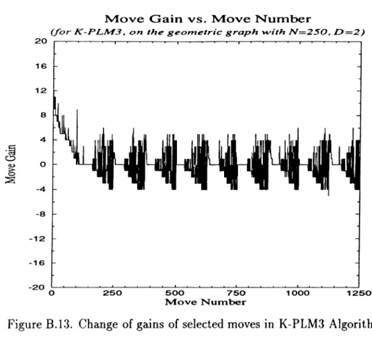
B.13 Change of gains of selected moves in K-PLM3 Algorithm . . . . 100

B.14 Change of cutsize at each move in K-PLM3 Algorithm (final cutsize is 0 ) ...100

List o f Tables

C.l Properties of Random Test G r a p h s ...102

C.2 Properties of Geometric Test G r a p h s ...102

C.3 Properties of Grid Test G r a p h s ... 102

C.4 Properties of Ladder Test G r a p h s ... 103

C.5 Properties of Tree Test Graphs ... 103

C.6 Properties of Benchmark Circuits (multiply wt by 1000, Cmax = 1 and Cmin = 1 for all c irc u its )...103

C.7 Execution time averages (and standard deviations) for random g r a p h s ... 104

C.8 Outsize averages (and standard deviations) for random graphs . 105 C.9 Execution time averages (and standard deviations) for geometric g r a p h s ... 106

C.IO Outsize averages (and standard deviations) for geometric graphs 107 0.11 Execution time averages (and standard deviations) for grid graphslOS 0.12 Outsize averages (and standard deviations) for grid graphs . . . 109

0.13 Execution time averages (and standard deviations) for ladder g r a p h s ... 109

0.14 Outsize averages (and standard deviations) for ladder graphs . . 110

C.15 Execution time averages (and standard deviations) for tree graphsl 10

LIST OF TABLES XV

C.16 Outsize averages (and standard deviations) for tree graphs . . . 110

CM7 Outsize averages for random graphs (with different freedom value functions for K -P F M l)...I l l

0.18 Outsize averages for random graphs (with different freedom value functions for K -P F M 2 )...I l l

0.19 Outsize averages for random graphs (with different freedom value functions for K -P F M 3 )... 112

0.20 Outsize averages for random graphs (optimizing S for K -PFM l) 112

0.21 Outsize averages for random graphs (optimizing S for K-PFM2) 113

0.22 Outsize averages for random graphs (optimizing S for K-PFM3) 114

0.23 Outsize averages for random graphs (for K-PLM-like algorithms) 115

0.24 Outsize averages for geometric graphs (for K-PLM-like algorithms) 115

0.25 Execution time averages (and standard deviations) for bench­ mark circuits ...116

0.26 Outsize averages (and standard deviations) for benchmark circu itsll?

0.27 Minimum Cutsizes for benchmark c i r c u i t s ... 118

0.28 Outsize averages for some benchmark circuits ... 118

LIST OF TABLES XVI

List o f Sym bols

M the set of natural numbers

A'(l,yV) every natural number between 1 and

o

G

H a hypergraph

V set of vertices

E set of edges (or nets)

V a vertex

e an edge (or a net)

d, degree of vertex u,

d{vi) degree of vertex V{

1^1 number of vertices in V

N

\E \ number of edges (or nets) in E

M number of edges (or nets) in E

P total number of terminals of nets in E

n a partition

K number of parts in a partition

Pk A:th part in a partition

w{v) weight of vertex v

c(e) weight of edge (or net) e

Wt total vertex weight

Ct total edge weight

D QXp expected average vertex degree before

Ddct actual average vertex degree after gene Dy^max maximum vertex degree (also £lv,x)

Dy average vertex degree

De,max maximum net degree (also £>e,i)

De average net degree

^max maximum vertex weight (also w^)

^min maximum vertex weight (also Wn)

^max maximum edge weight

LIST OF TABLES XVII

Ek set of external edges of part Pk

Ik set of internal edges of part Pk

x (n ) cutsize of partition fl

E m {f,t) external edges of vertex Vm € Pj with respect to

I m i f J ) external edges of vertex Vm € Pj

C M ^ t ) cost of vertex Vm € Pj with respect to Pt move gain of vertex € Pj with respect to Pt

Si(k) number of terminals of net e, in part Pk

7i reduction in cutsize at the qih move in a pass

Q maximum number of moves in a pass

cr, (prefix) sum of the first q reductions in cutsize

g a i n s u m maximum prefix sum

freedom value of vertex € Pj with respect to

R constant used to make freedom value be in (0,1)

S scale factor

Gjriax maximum move gain

njn move count of vertex Vm

S a solution

N (s) neighborhood of solution s

X(s) cost of solution s

K - P L M multiple-way partitioning by locked moves

K - P F M multiple-way partitioning by free moves

B (k) upper bound on size of part Pk

m lower bound on size of part Pk

a tolerance constant in balance condition

e a very small value greater than zero

s(Pk) size of part Pk

C h a p ter 1

IN T R O D U C T IO N

1.1

C o m b in a to ria l O p tim iz a tio n P rob lem s

Many problems that arise in practical situations are combinatorial optimiza­ tion problems which involve a finite set of configurations from which solutions satisfying a number of rigid requirements are selected. The goal is to find a solution of the minimum or maximum cost (or the optimum cost) provided th at a cost can be assigned to each solution.

Many combinatorial optimizations problems are hard in the sense that they are NP-hard or harder [13]. There are no known deterministic polynomial time algorithms to find the optimal solution to any of those hard problems. The algorithms employing the complete enumeration techniques are not reasonable to use because the complexity of these techniques is usually exponential in the size of the problem and hence, they require a great amount of time to find the optimal solution for even very small problem instances. As a result, heuristic algorithms (or heuristics) that run in a low-order polynomial time have been employed to obtain good solutions to these hard problems, where, by a good solution, we mean a solution th at is hopefully close to the optimal solution to the problem.

The methods used for designing heuristic algorithms tend to be rather prob­ lem specific. Local search is one of the few general approaches to solving hard combinatorial optimization problems. Local search is based on trial and error method, which is probably the oldest optimization method.

cn

Before deriving a local search algorithm for a problem, a neighborhood structure for any solution must be chosen. For each potential solution to the problem, this structure specifies a neighborhood which consists of a set of solutions that are in some sense close to that solution. A rule as to how a neighbor solution can be generated by modifying a given solution is associated with the neighborhood structure.

Starting from some given initial solution, a local search algorithm tries to find a better solution which is a neighbor of the first. If a better neighbor is found, a search starts for a better neighbor of that one, and so on. Since the set of solutions is finite, this search must halt, that is, the local search algorithm must end at a locally optimum solution, which does not have a better neighbor solution. Local search algorithms are also called iterative improvement algo­

rithms because they iteratively improve an initial solution so as to find a locally

optimal solution.

Suppose that the problem is a minimization problem and so the smaller the cost of the solution found, the better the solution. The modification of a given solution to obtain a neighbor in the neighborhood of the given solution is called a move. If the move results in a neighbor with a better cost, the move is a downhill move. On the other hand, if the move results in a neighbor with a worse cost, the move is an uphill move. The bcisic local search algorithm employs only downhill moves.

1.2

G rap h and H y p erg ra p h P a r titio n in g P ro b lem s

Graph partitioning problem is an example of the problems to which the local

search method has been successfully applied. Given a graph, graph partitioning problem is concerned with finding a partition of the graph into a predetermined number of nonempty, pairwise disjoint parts such that the sizes of the parts are bounded and the total size, cutsize, of the edges in the cut, those edges th at connect different parts, is minimized. Graph partitioning problem is an NP-hard combinatorial optimization (minimization) problem [13].

The importance of the graph partitioning problem is mostly due to its con­ nection to the problems whose solutions depend on the divide-and-conquer paradigm [26]. A partitioning algorithm partitions a problem into semi­ independent subproblems, and tries to reduce the interaction between these

CHAPTER 1. INTRODUCTION

subproblems. This division of a problem into simpler subproblems results in a substantial reduction in the search space [34].

Graph partitioning has many important applications in various areas such as VLSI layout [2, 21, 22, 33, 40], mapping of computation to processors in a parallel computer environment [7, 8, 30], sparse matrix calculations [14, 15, 24], and so on. There are also some theoretical justifications for the usage of graph partitioning in VLSI layout. For example, it is shown that a provable good graph partitioning algorithm can be tailored into a provable good layout algorithm [2].

A hypergraph is a generalization of a graph such that an edge, called a net in a hypergraph, of a hypergraph can connect more than two vertices. Hypergraph

partitioning problem is exactly the same as graph partitioning problem except

that the structure to be partitioned here is a hypergraph. Since an edge in a graph can only connect two vertices, edges do not properly represent electrical interconnections. As a result, a hypergraph is better suited to electrical circuits in which some of the nets have three or more connected devices [32]. Hence, not surprisingly, hypergraph partitioning has important applications in VLSI layout [4, 9, 11, 12, 28, 35, 36]. The hypergraph partitioning problem is also NP-hard [13].

If a graph (hypergraph) is to be partitioned into more than two parts, then the problem is referred to as multiple-way graph (hypergraph) partitioning problem. When there is only two parts in the partition, the problem is called graph (hypergraph) bipartitioning problem.

1.3

P r e v io u s A p p roach es

Since both graph and hypergraph partitioning problems are unfortunately hard problems, we should resort to heuristics to obtain at least a near-optimal solu­ tion. The most successful heuristic algorithm proposed for graph partitioning problem is due to Kernighan-Lin [19]. Kernighan-Lin (KL) algorithm is a very sophisticated improvement on the basic local search procedure, involving an iterated backtracking procedure that typically finds significantly better solu­ tions [17].

CHAPTER 1. INTRODUCTION

Scliweikert-Kernighan [32]. KL algorithm uses a swap-neighborhood structure in which a neighbor of a given solution is obtained by interchanging a pair of vertices between two distinct parts in the solution. Given a graph (hypergraph) KL algorithm associates each vertex with a property called the gain of the ver­ tex which is exactly the reduction in the cutsize when the vertex is moved in the partition. The swap-neighborhood structure happens to increase the running time of KL algorithm since a pair of vertices must be found to interchange. Fiduccia-Mattheyses [12] introduces the move-neighborhood structure in which a neighbor of a given solution is obtained by moving a vertex from one part to another in the solution. They also devise a very sophisticated data struc­ ture called the bucket list data structure which reduces the time complexity of KL algorithm to linear in the size of the hypergraph by keeping the vertices in sorted order with respect to their gains and by making the insertion and deletion operations cheaper. Krishnamurthy [20] adds the level gain concept which helps to break ties better in selecting a vertex to move. The first level gain in Krishnamurthy’s (KR) algorithm is exactly the same as the gain in Fiduccia-Mattheyses’ (FM) algorithm. Sanchis [31] generalizes KR algorithm to a multiple-way partitioning algorithm. Note that all the previous approaches before Sanchis’ (SN) algorithm are originally bipartitioning algorithms. SN al­ gorithm is a direct multiple-way partitioning algorithm in which, at any time during iterative partitioning, a vertex can be moved into any of the parts in the partition. However, the move should be legal, that is, it should not violate the balance condition which imposes certain bounds on the sizes of the parts in the partition. SN algorithm exploits the local minimization technique of KL al­ gorithm, the move-neighborhood structure, balance condition, and bucket list data structure of FM algorithm, and the level gain approach of KR algorithm.

Now, since the minimization technique of KL algorithm is the basis of the many partitioning algorithms that have followed it, we explain this technique as it is used in Fiduccia-Mattheyses’ algorithm, that is, in terms of vertex moves. First, an initial partition is generated. The gains of the vertices are also determined. The first move includes the legal move of the vertex with the maximum gain. This vertex is then tentatively moved and locked. A locked vertex is set aside and not considered again until all the vertices are moved and locked once, which corresponds to a pass of the algorithm. After the first move, the next legal move with the maximum gain is moved and locked. This process goes in the same manner until the end of the pass. Note that there is a recorded sequence of the moves and their respective gains at the end of the first pass. At the end of the pass, a subsequence of moves from the recorded

CHÁPTím 1. INTRODUCTION

sequence that yields the maximum reduction in the cutsize is selected and realized permanently but starting with the first move in the recorded sequence. This operation is called the prefix sum calculation. Using the current partition obtained at that pass, another pass goes on in exactly the same manner. These passes are performed until there is not any improvement in the cutsize, which corresponds a locally minimum partition. Since a pass involv'es the move of each vertex once, there may exist uphill moves during the pass. The permission of uphill moves in a pass makes this minimization technique better.

All the previous partitioning algorithms use the minimization technique above. Vijayan [40] extends this technique so that a vertex is not locked as soon as it is moved. The vertex is allowed to reside in each part once before it is locked.

Henceforth when we say that a move is selected, we mean that the move is performed or the vertex associated with the move is actually moved. In other words, selecting a move has the same meaning as performing a move.

1.4

M o tiv a tio n

When we examine the Kernighan-Lin’s minimization technique, it reveals that moves with positive gains, those that decrease the cutsize, become more useful during the early stages of the sequence of the moves performed during a p«iss and that moves with negative gains, those that increase the cutsize, become more useful towards the end of the sequence of the moves performed during a pass. Hence, we should perform as more moves with positive gains as we can during a pass as long as this process does not lead us to become stuck in a poor local minimum. After some experimentation, we can observe that moves with positive gains, especially those performed in the first péiss, occur actually during the early stages of the move sequence. However, we can also observe that, after some point in a pass, the moves that are selected to be moved mostly consist of those with negative gains. Experiments indicate that a move performed at an earlier stage in a pass can have positive gain again in a later stage such that its move gain is larger than those of the moves remaining but it cannot be performed because it is locked. The rea.son why this move is not performed has been to prevent the cell-moving process from thrashing or going into an infinite loop [12, 20, 40]. We think that this reason is not plausible

CHAPTER 1. INTRODUCTION

because we can find some other means to avoid thrashing or infinite number of moves during partitioning. Therefore, we make the following claim, on which all our work is based. Our claim states that given a hypergraph with N vertices,

allowing each vertex to be moved (possibly) more than once in a pass with the requirement that the occurrence of infinite number o f moves having no profit be prevented improves the cutsize more than allowing each vertex to be moved exactly once in a pass.

We bring the move-and~lock phase concept for the sake of simplicity of the discussion of this claim. A move-and-lock phase contains a sequence of temporary moves and their respective locks. A pass may consist of one or more move-and-lock phases. If a move-and-lock phase is not the last one in a pass, then all the vertices that are temporarily moved during this phase are unlocked and reinserted into the appropriate bucket lists, according to their recomputed gains, for the succeeding move-and-lock phases in that pass. On the other hand, if a move-and-lock phase constitutes the last such phase in a pass, the prefix subsequence of moves which maximizes the prefix sum of move gains in that pass is realized permanently. We now propose three novel approaches exploiting the basic claim:

1. During a pass, we can make more than one move-and-lock phase such that each move-and-lock phase consists of N moves.

2. During a pass, we can make more than one move-and-lock phase such that each move-and-lock phase consists of less than N moves.

3. During a pass, we can make more than N moves but we do not employ the locking mechanism at all. Yet, there should still be some means to restrict the repeated selections of moves.

We considered all of these ways for partitioning. The items (1) and (2) es­ tablish the basis of multiple-way partitioning-by-locked-moves method, which also subsumes SN algorithm, (in Section 4.11) and the item (3) establishes the basis of multiple-way partitioning-by-free-moves method (in Section 4.12). Both of these methods are proposed and implemented in this work for graph partitioning as well as hypergraph partitioning. We expect that these methods explore the search space of the problem better.

1.5

E x p e r im e n ts an d R e s u lts

We evaluated the graph partitioning algorithms on the graph instances that were randomly generated using the algorithms in the literature. The types of graph instances included random, geometric, grid, ladder, and tree graphs. The random and geometric graphs are standard test beds for graph partition­ ing algorithms [17, 3]. The other types of graphs were used to evaluate the partitioning algorithms because the KL algorithm is observed to fail badly on these types of graphs [6, 15]. We evaluated the hypergraph partitioning algorithms on the real VLSI circuits which had been taken from ACM/SIGDA D esign Automation Benchmarks. We also did experiments to determine the best setting of the parameters in the proposed algorithms.

The proposed partitioning algorithms performed drastically better than SN algorithm, which is the best KL-like multiple-way partitioning algorithm at the moment, on both the graph and hypergraph instances. The results on the benchmark circuits correlate favorably with those in the existing partitioning literature.

C liA FT E R 1. INTRODUCTION 7

1.6

O u tlin e

We present some preliminaries from graph theory, a formal definition of the graph partitioning problem, and bcisic concepts related to graph partitioning and graph partitioning algorithms in Section 2. The analogous issues for hy­ pergraphs are given in Section 3. An explanation concerned with the local search technique which constitutes the basis for the algorithms we considered, th e previous approaches to the partitioning problem, a detailed investigation of the proposed algorithms and their analysis are all presented in Section 4. The following section. Section 5, includes the algorithms which were used to generate the graph instances, the details of each group of experiments that we conducted, and the results and general observations obtained from the re­ sults. Finally, the main conclusions are in Section 6. Since we still have a large num ber of tables and plots giving the results of the experiments although we skipped most of them, these tables are all given in appendices for the sake of clarity while presenting the text.

C h a p ter 2

G R A P H P A R T IT IO N IN G

This chapter establishes the basic concepts on Graph Partitioning. It includes some preliminary concepts from graph theory, the definition of the graph par­ titioning problem, and the concepts related to the partitioning algorithms, which are examined in Chapter 4. We utilized the references [23, 38] for the definitions and notations.

2.1 In tr o d u c tio n

The importance of the graph partitioning problem is mostly due to its con­ nection to the problems whose solutions depend on the divide-and-conquer paradigm [26]. A partitioning algorithm partitions a problem into semi­ independent subproblems, and tries to reduce the interaction between these subproblems. This division of a problem into simpler subproblems results in a substantial reduction in the search space [34]. Graph partitioning is the basis of hypergraph partitioning, which is more general and more difficult. Graph partitioning has a number of important applications. An exhaustive list of these applications combined with the relevant references is given below.

• VLSI placement [2, 21, 22, 33].

• VLSI routing [40].

• VLSI circuit simulation [1, 10].

• mapping of computation to processors and load balancing [7, 8, 30].

• efficient sparse Gaussian elimination [14, 15, 24].

• solving various graph problems [25].

• laying out of machines in advanced manufacturing systems [39].

• computer vision [16].

Some researchers have also utilized the graph partitioning problem as a test bed to evaluate the search and optimization algorithms they proposed.

CHAPTER 2. GRAPH PARTITIONING 9

2.2

B a sic C o n c e p ts

A graph G = (y, E) consists of a finite set V of verfices (or nodes) and a finite set E of edges. Each edge is identified with a pair of vertices. We use the symbols u, V, vi,V2, · · · to represent the vertices and the symbols e, ej, C2, · · · to

represent the edges of a graph unless otherwise specified. The term graph here denotes undirected graphs, i.e., the edge e,· = {u,u} and the edge ej = {t»,u} represent the same edge.

Given an edge e = {u,u}, we say that the edge e is incident to its end vertices u and v, and th at the vertices u and v are adjacent or neighbors. If two edges have a common end vertex, then those edges are said to be adjacent.

The number of edges incident to a vertex u, is called the degree of the vertex and is denoted by ¿(u,) or simply d,. A vertex of degree 0 is called an isolated

vertex.

A graph G — (y, E) has | y |= A vertices and ] E\= M edges. Each vertex u in y has a positive integer weight w{v) {w for weight) and each edge e \n E has a positive integer weight c(e), (c for capacity).

Given a graph G = (K £·), we say that IT = (P i,---,P ft) is a K-way

partition of G if each part Pk is a nonempty subset of the vertex set y , all

the parts are pairwise disjoint, and the union of the K parts is equal to V. Formally, FI = (Pi, · · ·, Pfc) is a A-way partition of G = (E, P) if

CHAPTER 2. GRAPH PARTITIONING 10

2. Pjt n P/ = 0 for each k ,l e {1, · · ·, /i'} and {k ^ /),

3. u L . Pt =

y-Note that the number K of parts in a partition of G is bounded above by the number of vertices in G.

For simplicity, we say that i € A/”(Ni, A^2) if Ni < i < N2 and i, A^i, A^2 € jV"

where Ai is the set of natural numbers. Then, when we say that i 6 A/’(l, N) for a vertex v, in the vertex set V with N vertices, we mean that u,· is any vertex in V. Similarly, when we say that k 6 A i{ l,K ) for a part Pk in the /•i-way partition FI, we mean that Pk is any part in FI.

Consider a /t'-way partition FF = (Pj, · · ·, P/^-) of a graph G = {V^ E) with

N vertices and M edges. Then,

• s[Pk) denotes the size of the part Pjt for ^ € .^(1, K). The size of the part Pfc equals the sum of the weights of the vertices in Pjt. That is.

v€Pk

(2.1)

• The total vertex weight wt is the sum of the weights of all the vertices in the vertex set V. That is.

K WT = X )u;(u) = Y s { P k ) .

v£V k=l

(

.

)

• The total edge weight c j is the sum of the weights of all the edges in the edge set E. That is,

CT = E <'=)■ (2-3)

eeE

• € P I e = {u,u} A € F A u € Pjt A u ^ Pk} is the set of

external edges of the part Pk for all k 6 A i{ \,K ). The set of external

edges of a part Pk consists of those edges whose one end vertex lies in the part Pk and the other end vertex lies in another part in the partition FF.

• /* = {e € P I e = {u,u} Am,u € F A u,u € Pk} is the set of internal

edges of the part Pk for all k € A/’(l, K ). The set of internal edges of a

СНА PTER 2. GRA PH PA RTITIONING 11

• The edges that connect dilTerent parts in the partition IT, that is, the external edges, are said to contribute to the cut or cross the cut.

• The cost x(IT) of the partition is also called the cutsize. The cutsize is

the sum of the weights of all the edges contributing to the cut. That is.

х ( п ) = 5 1 ; E Ф ) . ^ k=i ceEk or к х(П) = ст - x ; x ; c(e). fc=le€/fc (2.4) (2-5)

• A K-vfa.y partition is also a multiple-way partition, and the partitioning operation is called K-way partitioning or multiple-way partitioning. If there are only two parts, i.e., K = 2, then FI is called also a bipartition or a 2-way partition.

• A partition is balanced if the parts have about the same size. A partition

is perfectly balanced if the parts have exactly the same size. A perfectly balanced partition is highly unlikely in a multiple-way partitioning if the vertex weights are not equal.

• The average (vertex) degree Dy of the graph G can be found by the equation

Dy = 2M

N

(

.

)

where 2M is equal to the sum of the degrees of all the vertices in G.

• The maximum (minimum) vertex degree of the graph G is the maximum

(minimum) of the set of the degrees of the vertices in G and is denoted

b y Dy,max { D v,min)·

• The maximum (minimum) vertex weight is the maximum (minimum) of the set of the weights of the vertices in G and is denoted by Wmax (tUmin)· The maximum (minimum) edge weight is the maximum (minimum) of the set of the weights of the edges in G and is denoted by с^ах (cm.n)·

2.3

G raph P a r titio n in g P ro b lem

A formal definition of the Graph Partitioning Minimization Problem (GPP) is given below. In this definition, an instance is obtained by specifying particular values for all the problem parameters.

CHAPTER 2. GRAPH PARTITIONING 12

P ro b le m : The Graph Partitioning Minimization Problem.

In sta n ce : A graph G = (V, E), a vertex weight function w : V Af, an edge

weight function c: E Af, a number K > 2, A' G maximum and minimum part sizes B{k) G A/" and b{k) G A/*, respectively, for k G A/*(l, K ).

C o n fig u ratio n s: All A'-way partitions fl = (Pi, · · ·, Pa )·

S olutions: All feasible configurations, i.e., all K-way partitions FI = (P i, · · ·, Pa)

such that

b{k) < s{Pk) < B{k) for all k G .V (l, K )

Q uestion: Find a solution such that the cutsize

x (n ) = i E E <<^)

^ Jt=l e€£*

is minimum over all the solutions.

Intuitively, we are given a graph G = (V ,E ). Each vertex and each edge have a positive weight. Each K-vf&y partition If = (Pi, · · ·, P/^-) of the vertex set V into nonempty, pairwise disjoint parts Pk (for k G A/^(l, A')), is a configu­ ration. Given an upper bound B{k) and a lower bound h{k) on the size of each part Pfc, we regard as solutions those partitions (or feasible configurations) in which the size of each part Pjt is in the range between b{k) and B{k). We are then asked to find the partition (or partitions) that has the minimum cutsize over all the solutions.

The graph partitioning minimization problem is NP-hard [13]. In order to see how large the search space of GPP is, let us simplify the problem. Suppose that G = {V ,E) is a graph with N vertices each of which has unit weight, and that the number N of the vertices is a perfect multiple of the number K of partitions and so let N jK = s, i.e., each part has a part size of s. Then,

, / N ] r , . , n ( \ . , .

there are I I ways of choosing the first part, I I ways of choosing

\ ^ / , . V ^ A .

the second part, and so on. Since the ordering of the parts is immaterial, the number of feasible partitions is

m

(2.7)

For N = 100 and K = 2, the number of feasible partitions is greater than 10^^, and for N = 100 and K = 4, it is greater than 10'’''. Today, there are graph partitioning instances with N — 50000. Hence, it is clear that the number of feasible partitions is too large to search exhaustively.

CHAPTER 2. GRAPH PARTITIONING 1 3

2 .4

M u lt ip le-w ay G raph P a r titio n in g

2.4.1

G ain C on cep t

Let G = {V^E) be a graph with N vertices and IT = {Pi,· · · ■, Pk) a A'-way

partition of G. Let f , t Q A f { \ , K) be two numbers ( / represents the part

from which a vertex is moved, and t represents the part to which the vertex is

moved.) The cost Cm{f , t ) of a vertex in Pj with respect to a part Pt (m for moved vertex) is defined as

r ( f f ) = i if / 7^ <

"

1

(

.

)

where

Em{f, t) = {e e Ef \ e = u} Au e Pt} (2.9) is the subset of the set of the external edges of the part Pj whose one end vertex is and the other end vertex lies in the part Pt, and

Im{f , f) = { e e If \ e = {Um,n} A u e Pf] (2.10) is the subset of the set of the internal edges of the part Pj whose one end vertex is and the other end vertex lies in the part Pj. The edges in the sets

Em( f , t ) and I m{ f , f ) are called the external edges and internal edges of the

vertex Vm with respect to the part Pt, respectively.

The move gain Gm{f, t ) of the vertex Vm in the part Pj with respect to the part Pt is given by the equation

G „ U A = C M , t ) - c „ u , f ) . (

2

11

That is, the gain Gm{f, t ) of a vertex Vm in the part Pj with respect to the part Pt is the difference between the sum of the weights of the external edges of Vm. whose the other end vertex is in Pt and the sum of the weights of the internal edges of Vm- The gain of a vertex represents the decrease that results in the cutsize when the vertex is moved. The gain of a vertex with respect to the part where the vertex is present is zero.

In the A'-way partition, each vertex has K costs. These costs constitute the cost vector of the vertex. For each vertex Vm in Pj, the entry Cm{ f , f ) is the internal cost of Vm and the other (A" — 1) entries are the external costs of

CHAPTER 2. GRAPH PARTITIONING 14

Algorithm: Initial Cost Computation Algorithm

Input: a graph G = (V, E ) with N vertices, a i\-w ay partition IT = (P i, Output: vertices in V with all cost vectors computed

•,PA')ofG

1. for each vertex v, , where r,· E Pj and i G A/^(l, N ) , d o

1.1. for each part number t, where t G A^(l, A') do 1.1.1. let ^ 0 /* initialize the cost * / 1.2. e n d fo r

1.3. for each edge e = {i>, , u} do

1.3.1. find the part P< such that u G Pt 1.3.2. \ e t C M t ) ^ C m { f J ) - l · c { e ) 1.4. e n d fo r

2. eiid fo r

Figure 2.1. An algorithm for initial cost computation in a graph

Figure 2.1 illustrates the pseudocode for the algorithm which computes the initial cost vectors of the vertices in a graph assuming an initial feasible partition. Note that the computation of the initial gains of the vertices can be done easily by using Equation 2.11 provided that the initial costs are given.

2 .4 .2

E ffects o f a V e r te x M ove

Let G = (V, E) be a graph and FI = (Pi, · · ·, Pk) a A'-way partition of G. Let

/ , i € A f { l , K ) be two numbers. Consider the move of the vertex in the part Pf to the part Pt, where f We now give the effects of this move.

1. E ffect on C u tsize : The cutsize should be updated by the equation

x { n ) ^ x { n ) - G m{ f . t ) (2.12)

where Gm{fi 0 vertex Vm before the move. Hence, the decrease

in the cutsize is equal to Gmifit)·, which is expected by the definition of the gain concept. Note that a negative gain value (i.e., Gm{f, t) < 0) increases the cutsize.

2 . E ffe c t o n P a r t S iz e s : T he part size of the part Pj decreases and the part size of th e part Pt increases by the m ove of Vm- Hence, T h e following changes

CHAPTER 2. GRAPH PARTITIONING 15

in the parts sizes should be done.

s(P)) t - s{Pj) - s{P,) <- s(P |) +

(2.13)

(2.14)

3. E ffect on V e rte x M oved : There is no change in the entries of the cost vector of the vertex Vm, which is moved. The only change in the cost vector is in the interpretation of some entries. The entry C m (/,/) was the internal cost of v,n before the move and the entry was the external cost of u„, to the part Pt before the move. After the move, the entry Cm{t,t) becomes the internal cost of Vm and the entry Cm{E f ) becomes the external cost of t»,,, to the part Pj where C m { f i f ) before the move is equal to Cm{tif) after the move and C m if ii) before the move is equal to after the move. However, since the internal cost of Vm is changed, the gains of to every part (other than Pt) in n must be recomputed using Equation 2.1 1.

4. E ffect on N e ig h b o r V ertices : The algorithm in Figure 2 . 2 calculates the changes in the costs and gains of the neighbor vertices that result from the vertex moved. The move of the vertex from the part Pj to the part

Pt affects only the costs C'r(^,/ ) and Cr{k,t) of a vertex Vr € Pk adjacent to Vm- li k ^ f and k ^ t, this means that there is no change in the internal

cost Cr{k,k) and hence, only two gain values G r { k ,f ) and Gr{k,t) should be updated using Equation 2.1 1. However, if either k = f or k = t, this means th at there is a change in the internal cost of Vr and hence, all the gain values for all the moves of Vr from Pk to all the other parts in the partition should be recomputed using Equation 2.11.

It should be noted that partitioning algorithms existing in the literature lock the vertex moved, thus preventing the further moves of such vertices. In such algorithms, the gain updates mentioned in the item (3) should not be considered at all. Similarly, the cost and gain updates mentioned in the item (4) should be considered only for the unlocked vertices adjacent to the vertex moved. However, one of the proposed algorithms (to be discussed later) does not lock a vertex after it is moved, and <issociates an attribute, referred here as the freedom value, with each vertex. This freedom value is a function of the current gain of a vertex. Thus, an update in the gain of a vertex results in an update in the freedom value of that vertex. The gain updates in the item (3) and the cost and gain updates in the item (4) should be carried out for the vertex moved and all its neighbor vertices in the proposed algorithm.

CHA PTER 2. GRA PH PA RTITIONING 16

Algorithm: Gain Update Algorithm

Input: a graph G = (K with N vertices, a A"-way partition 0 = (Pi, · ·, Pk) of G, move of Vm 6 Pj to P<

Output: updated costs and gains of neighbors of v,rx 1. for each edge e incident to Vm do

1.1. find Vr G Pk such that e = and P^ G 0 1.2. letG,(fc,/)-Gr(ib,/)-c(e)

1.3. let Cr{k,t) Cr{k, t)c{e)

1.4.

if

1.4.1. update only Gr{k^f) 1.4.2. update only Gr(Jt, <)

1.5. else /* there is change in internal cost of neighbor vertex */

1.5.1. update all (K — 1) gains of iv> 1·^·, all gains other than Gr{k,k) 1.6. endif

2. eiidfor

Figure 2.2. An algorithm for gain updates in a graph

2 .4 .3

B a la n c e C o n d itio n s

It is possible that the total weight w j of all the vertices is not a perfect multiple of the number of parts. Even if there is a partition where the part sizes are the same, the balance on the part sizes is broken with the first move. In addition, if the vertices do not have the same weight, then it is also a hard problem to divide these vertices into parts such that the sum of the pairwise differences between the part sizes is minimized. Therefore, some changes in the part sizes should be tolerable. This tolerance is established by means of imposing lower and upper bounds on the part sizes. These bounds constitutes the balance

condition.

The main idea behind any balance condition should be that, during the course of the graph partitioning algorithm, there always exists at least one vertex to move without violating the balance condition and that the move is not exactly the opposite of the previous move [20]. This idea is good but it may be difficult to guarantee it.

Now, we define our balance condition: Let G = {V,E) be a graph and IT = {Pi, · · ·, Pk) a K-way partition of G. Then, we have b{k) < s{Pk) < B{k) for each Pf. in TI by the definition of the graph partition problem. What remains

CHAPTER 2. GRAPH PARTITIONING 17

is to specify the values of these lower and upper bounds. We define

m = L ^ ( l - a )J

and

m = \ Y { l + a ) ]

(2.15)

(2.16)

where a , ( 0 < a < 1), is a constant. Thus, we allow a part size to be 100«% more or 1 0 0«% less than its value in a perfectly balanced partition. Moreover, during initial partitioning, we can increase a to relax the balance condition. We call a move legal if it does not violate the balance condition [.31].

C h ap ter 3

H Y P E R G R A P H P A R T IT IO N IN G

This chapter establishes the underlying concepts for Hypergraph Partitioning. It includes some preliminary concepts from hypergraph theory, the definition of the hypergraph partitioning problem, and the concepts related to the par­ titioning algorithms, which are examined in Chapter 4. We utilized the refer­ ences [23, 38] for the definitions and notations.

3.1

In tro d u ctio n

The applications of the Hypergraph Partitioning Problem can be listed exhaus­ tively as follows:

• VLSI placement [4, 9, 1 1, 1 2, 28, 35, 36].

• VLSI routing [4, 28].

VLSI circuit simulation [27, 37, 41].

3.2

B asic C o n cep ts

A hypergraph H — {V., E) consists of a finite set V of vei'tices (or cells) and a finite set £■ C 2'^ of hyperedges (or nets), where 2^ is the power set of the vertex set V. Each net e in £ is a subset of V. The elements of a net e in are called its terminals. We use the symbols u, u,ui, U2i ’ ' ’ represent the vertices and

CUA PTER 3. H YPERCRA P / i PA RTITIONING 19

the symbols c, ei, 6 2, · · · to represent the nets of a hypergrapli unless otherwise specified.

Given a net e in E, we say that the net e is incident to the vertex v if •u € e, and that the terminals of the net e are adjacent or neighbors. If a net e is incident to a vertex v then we say that the net e is on the vertex v and the vertex V is on the net e. A net with two-terminals is called a two-terminal net and a net with more than two terminals is a multi-terminal net. Terminals are also called pins.

The degree of a vertex n, in V is equal to the number of nets incident to t;,· and is denoted by d(u,) or simply d,·. A vertex of degree 0 is called an isolated

vertex. The degree of a net e in is equal to the number of its terminals and is denoted by |e |. We assume that, for any net e in E, the degree |e |> 2.

A hypergraph H = [V, E) has | K |= vertices and | E |= A/ nets. Each vertex V in y has a positive integer weight w{v) and each net e in E has a positive integer weight c(e). The total number of terminals in H is denoted by

p which can be calculated by the equation

P = S |e | e^E or (.3.1) (3.2) P = Y , d(v)· v€V

Note that M = 0{p) since every net is at least a two-terminal net. If we further assume that every vertex is contained in at least one net, namely, if the degree of each vertex is at least 1, then we have N = 0{p). The latter assumption is not imposed unless otherwise specified.

A graph G = (V, E) is also a hypergraph H = (K, E) with the property that every net in / / is a two-terminal net. That is, hypergraphs are generalization of graphs. If / / is a graph, the total number p of terminals in H becomes equal to 2M, where M is the number of nets in H.

Given a hypergraph H = (V, E), we say that FI = (Pi, · · ·, Pk) is a K-way

partition of H if each part Pk is a nonempty subset of the vertex set K, all

the parts are pairwise disjoint, and the union of the K parts is equal to V . Formally, FI = (Pi, · · ·, Pk) is a K-way partition of H = (F, E) if

CHA FTEIt :i HYPERGRA PR PA RTITIONING 20

2. Pk n P/ = 0 for each k ,l E Af{ 1, K) and {k ^ /),

3- U L , Pi. = y

-Note that the number K of parts in a partition of / / is bounded above by the number of vertices in H.

Consider a /f-way partition IT = (Pi, · · ·, Pk) of a hypergraph H = (K, E)

with N vertices, M nets, and p terminals. For the sake of completeness, we repeat some definitions from Chapter 2. Then,

• s{Pk) denotes the size of the part Pk for k 6 A^(l, f\). The size of the part Pk equals the sum of the weights of the vertices in Pjt. That is,

4Ph) = v€Pk

The total vertex weight w j is defined as

(3.3)

K

W T = Y w{v) = Y s { P k ) .

v^V k=l

(3.4)

• The total net weight Ct is defined as

O T = Y c(e). eeE

(3.5)

• Pjt = {e € P I e n Pjt / 0 A e — P)t ^ 0} is the set of external nets of the part Pk for all k € A )· The set of external nets of a part Pk consists of those nets that have at least one terminal in Pk and at least one terminal in another part in the partition 0 .

• /jt = {e € P I e n Pit ^ 0 A e — Pjt = 0} is the set of internal nets of the part Pk for all k € ^/"(1, K). The set of internal nets of a part Pk consists of those nets that have all its terminals in Pk.

• 6{{k) =1 {y € e, I y € Pit) I is the number of terminals of the net e, that are present in the part

Pk-• If there are k parts such that a net e has at least one terminal in each of these parts, the net e is said to connect k parts in the partition. •

• The nets that connect different parts in the partition 0 , that is, the external nets, are said to contribute to the cut or cross the cut.

CHAPTER 3. HYPERGRAPH PARTITIONING 2 1

• The cost с(П) of the partition is also called the cutsize. The cutsize is the sum of the weights of all the nets contributing to the cut. That is,

Х(П) = cr - X; X; c(e). (3.6)

/:=! e€/jk

Each net e crossing the cut contributes an amount of c(e) to the cutsize regardless of the number of parts that e connects. However, this is not the only possible definition of the cutsize for hypergraphs. For example, if the net e connects k parts then e can contribute an amount of [k — l)c(e) to the cutsize. Note that Equation 3.6 reduces to Equation 2.4 when / / is a graph.

• A K-'N&y partition is also a multiple-way partition, and the partitioning operation is called K-way partitioning or multiple-way partitioning. If there are only two parts, i.e., K = 2, then П is called also a bipartition or a 2-way partition.

• We say that a partition is balanced if the parts have about the same

size. A partition is perfectly balanced if the parts have exactly the same size. A perfectly balanced partition is highly unlikely in a multiple-way partitioning if the vertex weights are not equal.

• The average vertex degree of the hypergraph H can be found by the equation

D. = (3.7)

The average net degree De of the hypergraph / / can be found by the equation

D. = ^ . (.3.8)

Hence, the following equation holds:

D J I = D , N (3.9)

• The maximum (minimum) vertex degree of the hypergraph H is the maximum (minimum) of the set of the degrees of the vertices in / / and is denoted by Dy^max {Dv,min)· The maximum (minimum) net degree of

H is the maximum (minimum) of the set of the degrees of the nets in П

and is denoted by T>e,m«x (T>e,mm)·

• The maximum (minimum) vertex weight is the maximum (minimum) of the set of the weights of the vertices in H and is denoted by u'max (ii-’,,,,,,). The maximum (minimum) net weight is the maximum (minimum) of the set of the weights of the nets in II and is denoted by c„,ax (<%„,„).

CHAPTER 3. HYPERGRAPH PARTITIONING 2 2

3.3

H ypergraph P a r titio n in g P ro b lem

A formal definition of the Hypergraph Partitioning Minimization Problem (HPP) is given below.

P ro b le m : The Hypergraph Partitioning Minimization Problem.

In sta n ce : A hypergraph H = {V, E), a vertex weight function w : V Af,

a net weight function c : E Ai, a number K > 2, K £ Ai, maximum and

minimum part sizes B{k) € Af and b{k) € Af, respectively, for k £ Af{l, K). C onfigurations: All A'-way partitions H = (Pi, · · ·, Pk)·

S olutions: All feasible configurations, i.e., all /iT-way partitions H = (P i, · · ·, P/,-) such that

b{k) < s{Pk) < B{k) for all k e A i { l , K)

Q uestion: Find a solution such that the cutsize

X(H) = CT - X ; X ; c(e)

k=i eelk

is minimum over all the solutions.

Intuitively, we are given a hypergraph H = (V, E). Each vertex and each net have a positive weight. Each K-way partition H = (Pi, - - - , Pa') of the

vertex set V into nonempty, pairwise disjoint parts P^, (for k € A/’( l , / \ ) ) , is a configuration. Given an upper bound B{k) and a lower bound b{k) on the size of each part Pk, we regard as solutions those partitions in which the size of each part Pk is in the range between b{k) and B{k). We are then asked to find the partition (or partitions) that has the minimum cutsize over all the solutions.

The hypergraph partitioning minimization problem is NP-hard [13]. Since graphs are special versions of hypergraphs, GPP is a special version or a re­ stricted version of HPP. Any partitioning algorithm that can produce a solution to HPP can produce a solution to GPP without any modifications in the algo­ rithm. However, an algorithm for GPP may not be used for HPP. Some parts of the algorithm need to be altered.

Additional constraints [29] that can be imposed in HPP are itemized below.

• The number of parts in a partition is minimized provided that there are bounds on the part sizes.

CHAPTER 3. HYPERGRAPH PARTITIONING 23

• The total number of external nets of each part is bounded.

• A certain set of nets must contribute to the cut.

• A certain set of nets must not contribute to the cut.

The algorithms we investigated can be modified to handle these constraints without too much additional effort. We did not consider to meet these con­ straints, however.

3.4 M u ltip le-w a y H ypergraph P a r titio n in g

3.4.1

G ain C on cep t

Let H = (V,E) be a hypergraph with N vertices and IT = (P\,· · ·, Pk) a,

A-way partition of H. Let f , t E A f{ \ , K ) be two numbers ( / represents the part from which a vertex is moved, and t represents the part to which the vertex is moved.) The cost Cm{fi t) of a vertex Vm in Pj with respect to a part

Pt {m for moved vertex) is defined as

^ ( f . ) _ ! Е е е а д ,о < е ) i i f ^ t

1

(3.10)

(3.11) = (e, e Ey I !>„ € e,· A Si{t) = |e , | -1 }

is the subset of the set of external nets of the part Pj whose one terminal is

Vjn and all the other terminals lie in the part Pt, and

= {e,· € / / 1 v,n € e,· Л Si{f) = |e ,|} (3.12) is the subset of the set of internal nets of the part Pf whose one terminal is and all the other terminals lie in the part Pf.

The move gain G ,„(/, t) of the vertex Vm in the part Pj with respect to the part Pi is given by the equation

(3.13)

That is, the gain G,n{f,t) of a vertex in the part Pj with respect to the part Pt is the difference between the sum of the weights of the nets who.se the