Published online in Wiley Online Library (wileyonlinelibrary.com) DOI: 10.1002/met.1575
Downscaling of monthly precipitation using CMIP5 climate models operated
under RCPs
Umut Okkan
a,* and Umut Kirdemir
baDepartment of Civil Engineering, Balikesir University, Turkey bDepartment of Civil Engineering, Izmir Institute of Technology, Turkey
ABSTRACT:Downscaling of general circulation model (GCM) outputs extracted from CMIP5 datasets to monthly
pre-cipitation for the Gediz Basin, Turkey, under Representative Concentration Pathways (RCPs) was performed by statistical downscaling models, multi-GCM ensemble and bias correction. The output databases from 12 GCMs were used for the pro-jections. To determine explanatory predictor variables, the correlation analysis was applied between precipitation observed at 39 meteorological stations located over the Basin and potential predictors of ERA-Interim reanalysis data. After setting both artificial neural networks and least-squares support vector machine-based statistical downscaling models calibrated with determined predictor variables, downscaling models producing the most suitable results were chosen for each meteorologi-cal station. The selected downsmeteorologi-caling model structure for each station was then operated with historimeteorologi-cal and future scenarios RCP4.5, RCP6.0 and RCP8.5. Afterwards, the monthly precipitation forecasts were obtained from a multi-GCM ensemble based on Bayesian model averaging and bias correction applications. The statistical significance of the foreseen changes for the future period 2015–2050 was investigated using Student’s t test. The projected decrease trend in precipitation is significant for the RCP8.5 scenario, whereas it is less significant for the RCP4.5 and RCP6.0 scenarios.
KEY WORDS statistical precipitation downscaling; CMIP5 data; RCPs; ERA-Interim reanalysis data; multi-GCM ensemble; correcting bias
Received 23 November 2015; Revised 10 February 2016; Accepted 19 February 2016
1. Introduction
General circulation models (GCMs) can be taken into con-sideration to obtain climate change projections for hydro-meteorological variables. In spite of their practical usage, the main problem with the projections produced from GCMs is their coarse resolution. Therefore, downscaling strategies have been developed (Wilby and Wigley, 1997).
In the literature, downscaling methods have been classified into two groups: dynamical and statistical downscaling (Wilby et al., 1998). Dynamical downscaling is related to regional cli-mate modelling. Simulating local clicli-mate characteristics can be feasible using dynamical models (Leung et al., 2003), yet they have several drawbacks in terms of their demanding design and computational redundancy (Fowler et al., 2007).
Statistical downscaling methods are used to transform the outputs from GCMs to the local scale by means of mathe-matical relationships derived from different methods (Okkan and Inan, 2015a). These kinds of methods require less com-putational effort than dynamical downscaling applications and are considered to be the most practical downscaling tech-niques in the hydro-meteorology literature (Tripathi et al., 2006). Regression-based techniques (e.g. Wilby et al., 1998; Hessami et al., 2008), weather generator (Semenov, 2008) and artificial neural networks can be preferred. Successful downscaling stud-ies carried out with artificial neural networks (ANNs) under dif-ferent climate change scenarios can be found in the literature
* Correspondence: U. Okkan, Department of Civil Engineering, Hydraulic Division, Balikesir University, 10145, Balikesir, Turkey. E-mail: [email protected]
(Goyal and Ojha, 2012; Okkan and Fistikoglu, 2014; Okkan, 2015; Okkan and Inan, 2015b).
In spite of the many superiorities of ANNs, they also have drawbacks, including the local minima problem and complex-ity in determining layered architecture (Suykens, 2001). Sup-port vector machines (SVMs) and two-parameter version called least-squares support vector machines (LSSVMs) can be consid-ered as alternatives to ANNs without their disadvantages. SVMs and LSSVMs have shown remarkable results in statistical down-scaling content. In a study carried out by Tripathi et al. (2006), an LSSVM was applied to future forecasts from the CGCM2 to obtain future projections of monthly precipitation for the mete-orological sub-divisions in India. Similar methods were applied by Anandhi et al. (2008) to downscale precipitation to a study region in Karnataka State, India. A statistical downscaling strat-egy based upon a modified SVM model was developed by Chen et al. (2010) to forecast precipitation in a basin in China. Sachin-dra et al. (2013) employed an LSSVM for transforming GCM simulations to local scale flows observed in northwestern Victo-ria, Australia.
Many of downscaling studies mentioned above have consid-ered previous climate change scenarios, which are mentioned in the Intergovernmental Panel on Climate Change (IPCC)-Fourth Assessment Report (AR4) as the Special Report on Emis-sion Scenarios (SRES). However, the Fifth Assessment Report (AR5) of the IPCC published in 2014 provided new scenar-ios termed ‘Representative Concentration Pathways’ (RCPs). RCPs comprise groups of several scenarios that produce emis-sion pathways related to the future emisemis-sions of greenhouse gases, aerosols, ozone and land use/land cover changes, whereas AR4 scenarios (SRES) included only forcing by greenhouse gases and aerosols (Moss et al., 2010; Meinshausen et al., 2011).
Black Sea
Legend
Meteorological Stations
ERA-Interim Grid Centres
Lakes Streams N S W E TURKEY A egean Sea 0.75° 0.75° 27°0'0''E, 39°0'0''E,
27°0'0''E, 38°15'0''N, 27°45'0''E, 38°15'0''N, 28°30'0''E, 38°15'0''N, 29°15'0''E, 38°15'0''N, 29°15'0''E, 39°0'0''N, 28°30'0''E, 39°0'0''N 27°45'0''E, 39°0'0''N Buldah Dindarli Sarigöl Alasehir Kula Fakili Simav Saphane Godiz Selendi Demirci Hanya Gördes Kiran ih icikler Güre E mata köyü Gediz Basin s s s Borlu Demirköprü Köprüba i Y. Poyraz Kavakalan Gölmarmara Hacirahmanli Sanihanli Uçpinar Foça Menemen TS Muradiye Manisa Marmara GR Salihli Ahmetli Turgutlu Kemalpasa Akhisar Sarilar U aks s Av als
Figure 1. Location of Gediz Basin (Turkey), meteorological stations within the Basin and ERA-Interim grid coverage.
These emission pathways are classified with the radiative forcing
generated by the end of the 21st Century. In this context,
Cou-pled Model Inter-comparison Project Phase 5 (CMIP5) services datasets of new-generation GCMs under different RCPs.
More recently, several studies in the literature have adopted RCP scenarios to assess possible climatic change effects on hydrological variables. In a study presented by Chong-hai and Ying (2012), alteration in air temperature and precipitation over regions located in China were described based on the outputs
of various GCMs with projections of 21stcentury climate under
different RCP scenarios. Kim et al. (2013) examined the sep-arated and combined effects of probable changes in climate and land use/land cover on streamflow for the Hoeya Basin, South Korea, using two RCP scenarios. Ji and Kang (2013) used a dynamical downscaling model with two RCP scenarios to project precipitation and temperature over the Tibetan Plateau. Lee et al. (2014) presented another dynamical downscaling work about the evaluation of future climate change over East Asia considering two RCPs. Analysis of precipitation lapse rate over north Sikkim, eastern Himalayas, under RCPs was also performed by Singh and Goyal (2016).
The present study explores the potential of statistical down-scaling methods, evaluates the downscaled multiple GCMs with an ensemble approach and uses new scenarios for project-ing monthly precipitation over Gediz Basin in the Aegean region of Turkey. The explanatory predictor selection work is investigated prior to outlining the downscaling process. The potential predictor selection was provided from the monthly ERA-Interim reanalysis dataset. The calibrated and validated downscaling model structure was integrated to 12 GCMs with three RCP scenarios. The precipitation forecasts were obtained from multi-GCM ensemble through a Bayesian model averaging
method followed by correcting biases. The bias-corrected fore-casts produced for the near future period (2015–2050) were then examined to understand the probable climate change impacts on the precipitation regime.
To the best of our knowledge, a statistical downscaling study concerning the use of RCP scenarios for climate projections in Turkey has not been realized previously. Projected changes of hydrometeorological variables for different basins in Turkey under SRES of AR4 have been obtained from the simulation of GCMs in version three of the Coupled Model Inter-comparison Project, CMIP3 (e.g. Okkan and Fistikoglu, 2014; Okkan and Inan, 2015a, 2015b) However, in the present work, projections derived from statistical downscaling techniques are introduced based on CMIP5 data in the hope of providing a reference for investigating the probable climatic change impacts on the precipitation regime in the Basin under different RCPs.
The paper is structured in four sections. The properties of the study region, the reanalysis and GCM data, selection of the predictor and statistical downscaling techniques are presented in the next section. The results obtained are given in the third section, and the summary and conclusions form the concluding part of the paper.
2. Data and methodology
2.1. Study region and preparing data
The application area covers the Gediz Basin in Turkey, which is located in the Aegean Region (Figure 1). The Gediz River is the second-largest river in Turkey flowing into the Aegean Sea.
The total drainage area of the Basin is 17 125 km2. The Basin
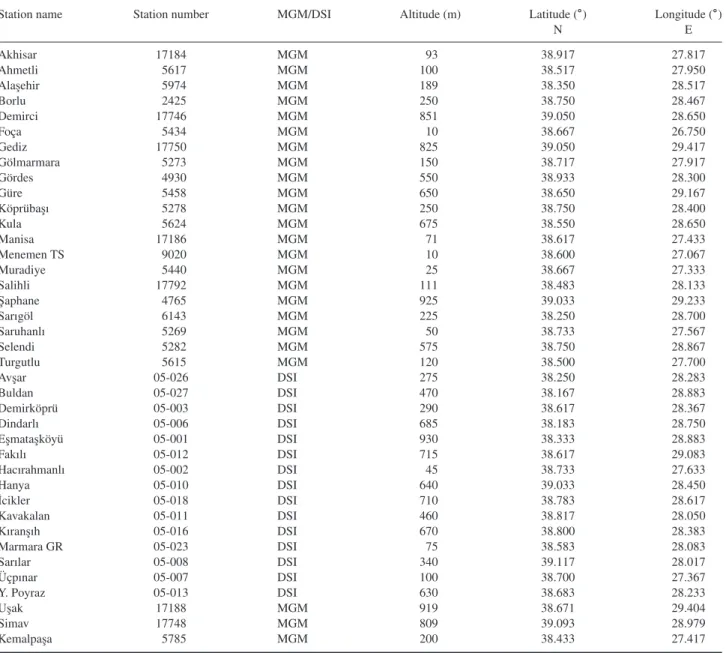
Table 1. Meteorological stations in the Gediz Basin, Turkey, where observed precipitation data were used for the downscaling exercise.
Station name Station number MGM/DSI Altitude (m) Latitude (∘) Longitude (∘)
N E Akhisar 17184 MGM 93 38.917 27.817 Ahmetli 5617 MGM 100 38.517 27.950 Ala¸sehir 5974 MGM 189 38.350 28.517 Borlu 2425 MGM 250 38.750 28.467 Demirci 17746 MGM 851 39.050 28.650 Foça 5434 MGM 10 38.667 26.750 Gediz 17750 MGM 825 39.050 29.417 Gölmarmara 5273 MGM 150 38.717 27.917 Gördes 4930 MGM 550 38.933 28.300 Güre 5458 MGM 650 38.650 29.167 Köprüba¸sı 5278 MGM 250 38.750 28.400 Kula 5624 MGM 675 38.550 28.650 Manisa 17186 MGM 71 38.617 27.433 Menemen TS 9020 MGM 10 38.600 27.067 Muradiye 5440 MGM 25 38.667 27.333 Salihli 17792 MGM 111 38.483 28.133 ¸Saphane 4765 MGM 925 39.033 29.233 Sarıgöl 6143 MGM 225 38.250 28.700 Saruhanlı 5269 MGM 50 38.733 27.567 Selendi 5282 MGM 575 38.750 28.867 Turgutlu 5615 MGM 120 38.500 27.700 Av¸sar 05-026 DSI 275 38.250 28.283 Buldan 05-027 DSI 470 38.167 28.883 Demirköprü 05-003 DSI 290 38.617 28.367 Dindarlı 05-006 DSI 685 38.183 28.750 E¸smata¸sköyü 05-001 DSI 930 38.333 28.883 Fakılı 05-012 DSI 715 38.617 29.083 Hacırahmanlı 05-002 DSI 45 38.733 27.633 Hanya 05-010 DSI 640 39.033 28.450 ˙Icikler 05-018 DSI 710 38.783 28.617 Kavakalan 05-011 DSI 460 38.817 28.050 Kıran¸sıh 05-016 DSI 670 38.800 28.383 Marmara GR 05-023 DSI 75 38.583 28.083 Sarılar 05-008 DSI 340 39.117 28.017 Üçpınar 05-007 DSI 100 38.700 27.367 Y. Poyraz 05-013 DSI 630 38.683 28.233 U¸sak 17188 MGM 919 38.671 29.404 Simav 17748 MGM 809 39.093 28.979 Kemalpa¸sa 5785 MGM 200 38.433 27.417
Turkish State Meteorological Service (MGM); General Directorate of State Hydraulic Works (DSI).
The region includes broad irrigation plains with an area of nearly 110 000 ha where intensive agricultural practices are carried out. Grape, maize, cotton and various other fruits and vegetables are the main crops grown in the Basin. A major part of existing water resources is used for irrigation purposes because agriculture is the major economic activity in the region. The Demirkopru Dam located in the centre of the Basin has the largest reservoir and Marmara Lake is the other main water supply for irrigation. The other dams in the Basin have relatively small reservoirs.
The monthly precipitation data measured at the Basin were obtained from 39 meteorological stations for the period January 1980 to December 2005. The study area has a Mediterranean climate. The average temperature in summer in the basin varies from 23.5 to 25.5 ∘C, that of winter varies from 5.3 to 6.8 ∘C, and the mean annual temperature is 15 ∘C. The majority of measured rainfall is observed in the winter, whereas summer is much drier. The total annual areal precipitation calculated from the Thiessen polygon method is about 550 mm for the same period. In recent years, like many basins with Mediterranean climate characteris-tics, the Gediz Basin has suffered from water scarcity because of
drought resulting from decreased precipitation, increased tem-perature and rapid demographic development. Thus, projecting precipitation under different climate change scenarios is impor-tant for water resource planning in this region of Turkey.
The observed monthly precipitation records at 39 meteorologi-cal stations located in the Gediz Basin (Figure 1; station numbers and their geographical coordinates are given in Table 1) were used for the statistical downscaling exercise. The station records were provided from the Turkish State Meteorological Service (MGM) and General Directorate of State Hydraulic Works (DSI). Monthly precipitation data of each station from January 1980 to December 2005 were considered as the predictand, whereas ERA-Interim monthly reanalysis data from the European Centre for Medium-Range Weather Forecasts (ECMWF) were selected as potential predictor variables for the observation period.
ERA-Interim reanalysis data have been used frequently as pos-sible predictors for downscaling in the literature (Bürger et al., 2012; Haas and Pinto, 2012; Vu et al., 2015). The variables of the determined eight ERA-Interim grids (Figure 1) cover-ing the basin, with latitudes 37.875–39.375 ∘ N and longitudes
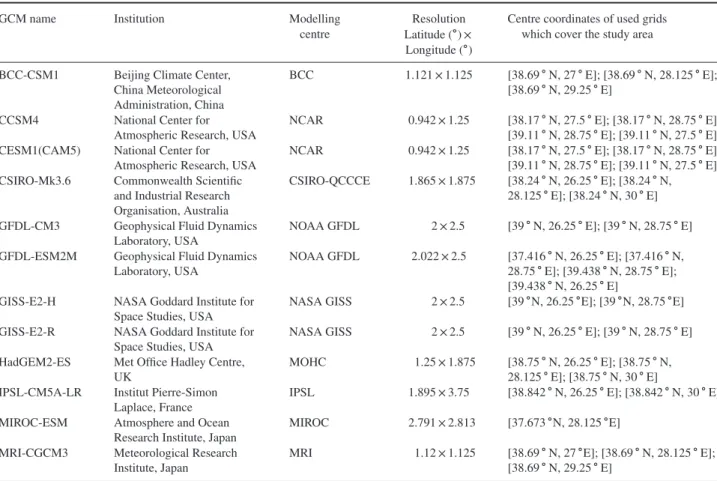
Table 2. Information about selected general circulatin models (GCMs).
GCM name Institution Modelling
centre
Resolution Centre coordinates of used grids which cover the study area Latitude (∘) ×
Longitude (∘) BCC-CSM1 Beijing Climate Center,
China Meteorological Administration, China
BCC 1.121 × 1.125 [38.69 ∘ N, 27 ∘ E]; [38.69 ∘ N, 28.125 ∘ E]; [38.69 ∘ N, 29.25 ∘ E]
CCSM4 National Center for Atmospheric Research, USA
NCAR 0.942 × 1.25 [38.17 ∘ N, 27.5 ∘ E]; [38.17 ∘ N, 28.75 ∘ E]; [39.11 ∘ N, 28.75 ∘ E]; [39.11 ∘ N, 27.5 ∘ E] CESM1(CAM5) National Center for
Atmospheric Research, USA
NCAR 0.942 × 1.25 [38.17 ∘ N, 27.5 ∘ E]; [38.17 ∘ N, 28.75 ∘ E]; [39.11 ∘ N, 28.75 ∘ E]; [39.11 ∘ N, 27.5 ∘ E] CSIRO-Mk3.6 Commonwealth Scientific
and Industrial Research Organisation, Australia
CSIRO-QCCCE 1.865 × 1.875 [38.24 ∘ N, 26.25 ∘ E]; [38.24 ∘ N, 28.125 ∘ E]; [38.24 ∘ N, 30 ∘ E] GFDL-CM3 Geophysical Fluid Dynamics
Laboratory, USA
NOAA GFDL 2 × 2.5 [39 ∘ N, 26.25 ∘ E]; [39 ∘ N, 28.75 ∘ E] GFDL-ESM2M Geophysical Fluid Dynamics
Laboratory, USA
NOAA GFDL 2.022 × 2.5 [37.416 ∘ N, 26.25 ∘ E]; [37.416 ∘ N, 28.75 ∘ E]; [39.438 ∘ N, 28.75 ∘ E]; [39.438 ∘ N, 26.25 ∘ E]
GISS-E2-H NASA Goddard Institute for Space Studies, USA
NASA GISS 2 × 2.5 [39 ∘N, 26.25 ∘E]; [39 ∘N, 28.75 ∘E] GISS-E2-R NASA Goddard Institute for
Space Studies, USA
NASA GISS 2 × 2.5 [39 ∘ N, 26.25 ∘ E]; [39 ∘ N, 28.75 ∘ E] HadGEM2-ES Met Office Hadley Centre,
UK
MOHC 1.25 × 1.875 [38.75 ∘ N, 26.25 ∘ E]; [38.75 ∘ N, 28.125 ∘ E]; [38.75 ∘ N, 30 ∘ E] IPSL-CM5A-LR Institut Pierre-Simon
Laplace, France
IPSL 1.895 × 3.75 [38.842 ∘ N, 26.25 ∘ E]; [38.842 ∘ N, 30 ∘ E] MIROC-ESM Atmosphere and Ocean
Research Institute, Japan
MIROC 2.791 × 2.813 [37.673 ∘N, 28.125 ∘E] MRI-CGCM3 Meteorological Research
Institute, Japan
MRI 1.12 × 1.125 [38.69 ∘ N, 27 ∘E]; [38.69 ∘ N, 28.125 ∘ E]; [38.69 ∘ N, 29.25 ∘ E]
26.625–29.625 ∘E, were compiled from the ECMWF website http://apps.ecmwf.int/datasets/. Each grid presented in Figure 1 has a spatial resolution of 0.75∘. Thus, a box covering the basin was obtained at a resolution of 1.5∘ × 3.0∘.
The large-scale output databases from 12 GCMs, which include both historical scenario outputs representing past climates and future climate simulations under the RCP4.5, RCP6.0, and RCP8.5 scenarios, were selected for the down-scaling exercise in the Basin under RCP scenarios. Another scenario, RCP 2.6, which is the most optimistic scenario in
terms of CO2emissions, was not examined in this study because
hydrometeorological tendencies observed in the Basin point out probable warming and water scarcity problems that could occur in the near future. In the present study, the 1980–2005 period was used for historical scenario simulations, whereas the 2015–2050 period was considered for RCP simulations. The selected RCPs represent different radiative forcing pathways from greenhouse gas emissions resulting from anthropogenic
actions, with radiative forcing of 4.5, 6.0 and 8.5 W m−2 by
2100, respectively. For the year 2100, the greenhouse gas con-centrations for RCP4.5, RCP6.0, and RCP8.5 are equivalent
to 650, 850 and >1370 parts per million CO2, respectively.
Compared to other RCPs, RCP8.5 corresponds to the pathway with the maximal greenhouse gas emission. It is assumed that excessive population and slow income growth with modest rates of technological change will be effective under RCP8.5 scenario (Riahi et al., 2011).
The CMIP5 set of experiments shares RCP simulations of various GCMs through several gateway websites operated by the Earth System Grid Federation (ESGF). In the study, the large-scale scenario outputs, which comprise both historical cli-mate and future simulations forced by RCPs, were extracted from
the gateway website http://pcmdi9.llnl.gov/esgf-web-fe/. Infor-mation about selected GCMs and the centre co ordinates of the grids covering the study region are given in Table 2.
In this study, 11 ERA-Interim variables, which were com-mon to data involved in 12 GCMs having 3 RCP scenarios, were extracted with the intention of establishing statistical down-scaling models based on ANN/LSSVM techniques to transform GCM outputs to the monthly precipitation for 39 meteorologi-cal stations. The dataset consists of several variables including mean air temperature (air), geo-potential height (hgt) and rela-tive humidity (rhum) at different atmospheric levels (200, 500 and 850 hPa), large-scale precipitation (pr) and sea-level pressure (slp) at Earth’s surface, which are the probable predictor vari-ables. An interpolation procedure was also used to get the outputs of GCMs at reanalysis grid box consisting of eight ERA-Interim grids because the grid centers of employed GCMs may not be consistent with reanalysis grid center.
2.2. Predictor selection
In the statistical downscaling literature, exercises confirm that explanatory predictors can change from one location to another. Any predictor can be considered before the downscaling step, but only if it shows plausible correlation with the observa-tions (Fistikoglu and Okkan, 2011). Determining the predictors through correlation–regression analyses is frequently preferred (Hessami et al., 2008; Fistikoglu and Okkan, 2011), although the relationships between some variables can be nonlinear and selecting the predictors via linear regression-based techniques may not seem true at first sight. Wilby et al. (2002) also advised a predictor selection procedure through regression analysis within the context of some guidelines for scenario usage. There are
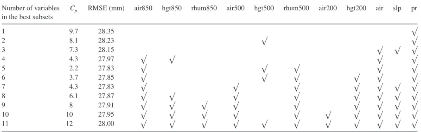
Table 3. Summary of All Possible Regression method (APREG) analyses for Manisa station. Number of variables
in the best subsets
Cp RMSE (mm) air850 hgt850 rhum850 air500 hgt500 rhum500 air200 hgt200 air slp pr
1 9.7 28.35 √ 2 8.1 28.23 √ √ 3 7.3 28.15 √ √ √ 4 4.3 27.97 √ √ √ √ 5 2.2 27.83 √ √ √ √ √ 6 3.7 27.85 √ √ √ √ √ √ 7 4.3 27.83 √ √ √ √ √ √ √ 8 6.1 27.87 √ √ √ √ √ √ √ √ 9 8 27.91 √ √ √ √ √ √ √ √ √ 10 10 27.95 √ √ √ √ √ √ √ √ √ √ 11 12 28.00 √ √ √ √ √ √ √ √ √ √ √
Air, mean air temperature (∘C); slp, sea level pressure (hPa); pr, large-scale precipitation (kg m−2); hgt, geo-potential height (m); rhum, relative humidity (%).
200, 500, and 850 near the variables denote the related atmospheric level (hPa).
various ways of determining predictors, too. The All Possible Regression method (APREG), which was also used in this study context, is another effective tool to determine the best subset of predictors (Fistikoglu and Okkan, 2011). In APREG applica-tion assessment of subset regression combinaapplica-tions can be based on conventional measurements such as the root mean squared
error (RMSE) and Mallows’ Cp co-efficient. Details about the
APREG procedure applied to downscaling studies were given by Fistikoglu and Okkan (2011) and Okkan and Fistikoglu (2014).
In the APREG application for this study, the monthly precip-itation values observed at 39 meteorological stations located in the basin were the predictand variables, whereas variables in the ERA-Interim reanalysis were the probable predictor data. The predictors are composed of the average of the values belonging to eight grids enclosing the basin. As a representative example, a summary of the results obtained from the APREG for Man-isa station is given in Table 3. According to Table 3, Mallows’
Cpco-efficient decreases rapidly up to five-regressor model and
then increases with the use of further variables. It can be said also that the large-scale pr variable of the reanalysis dataset, which appeared in all input combination as a predictor, increased the statistical relationship, confirming what other studies in the lit-erature have emphasized previously (Salathé, 2003; Tatli et al., 2004; Xoplaki et al., 2004; Schmidli et al., 2006).
The common belief is that the subset regression model with
the lowest RMSE and Cp should be chosen as the best one.
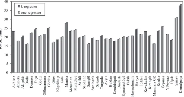
However, performances of k-regressor models having k predictor are nearly the same as that of the one-regressor model including only the pr variable; that is, the RMSE values calculated from one-regressor and k-regressor models are nearly equal for all stations. In other words, it can be observed that the change in RMSE is no longer meaningful when the number of predictors exceeds one (Figure 2). Thus, the predictor selection process determined the model with one variable as optimum, which implies that only large-scale pr is sufficient for the downscaling of monthly precipitation over the whole Basin.
2.3. ANN and LSSVM
One of the downscaling models used in this study is based on arti-ficial neural networks (ANNs). ANNs can be defined as a black box technique producing output against input(s) and is one of the preferred statistical downscaling techniques. Among various algorithms applied to a typical ANN structure composed of feed forward and back propagation steps, a second-order optimization
algorithm called the Levenberg–Marquardt algorithm (LM) is quite successful because it is generally faster and more suitable than other algorithms. Hagan and Menhaj (1994) presented a comprehensive description of ANNs with LM.
The Support Vector Machine (SVM) is another artificial intel-ligence algorithm constructed with statistical learning theory. Despite successful modelling performance of SVM, it has sev-eral disadvantages which were discussed in Suykens (2001). However, the least squares support vector machine (LSSVM) shows a computational benefit over the conventional support vec-tor machine method by transforming the quadratic optimization experience into a linear equation system. Tripathi et al. (2006) presented a detailed description of the LSSVM applied to down-scaling modelling.
2.4. Performance metrics for ANN/LSSVM models
Moriasi et al. (2007) indicated the significance of the use of three metrics, namely, Nash–Sutcliffe efficiency (NS), root mean squared error-observations standard deviation ratio (RSR) and bias percentage (PBIAS), to examine predicting capabilities. These metrics were also employed in this study for compar-ing two statistical downscalcompar-ing models, although originally they were intended for hydrological model assessment. The formula-tions of these metrics and ratings pertaining to metrics were given by Moriasi et al. (2007).
3. Results
3.1. Training and testing of statistical downscaling models
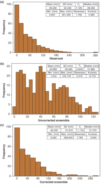
First, and before starting the downscaling modelling, all data were divided into two periods for application: the training period (January 1980 to December 1992) and the testing period (January 1993 to December 2005). The downscaling strategy proposed in this study was designed with a MATLAB code and summarized in Figure 3. In this study, all data were standardized before being input into two statistical models because z-score standardization makes the training of a downscaling model capable. This stan-dardization procedure also was applied to scenario data of GCMs as mentioned in Figure 3.
In the training period of the ANN/LSSVM using reanalysis data, estimation of optimal values for the related parameters were important. In the training of the ANN with the LM algorithm, the numbers of neurons in the hidden layer (n.n.h) made RMSE
Figure 2. RMSE statistics calculated from k-regressor and one-regressor models.
statistics the lowest were determined iteratively (Table 4). The parameters of the LM algorithm, which are the initial Marquardt
parameter (𝜇0) and decay rate (𝛽), were selected as 0.010 and
0.1, respectively. In addition, by monitoring the relative changes on RMSE statistics, the optimal epoch number could be chosen after several trials operated in the MATLAB-ANN toolbox.
The LSSVM model needs the calibration of two parameters:
the regularization parameter (𝛾) and the Gaussian radial basis
function (GRBF) width (𝜎). In the LSSVM training period, the
grid-search method under k-fold cross-validation was applied to estimate optimal LSSVM parameters (see Table 4), which made RMSE the lowest in the training. After different trials for this study, the number of folds was selected as 10. The grid search method can yield an optimal parameter set and employing a cross-validation procedure can prevent the downscaling model from over-fitting. The authors refer readers to a MATLAB tool-box available at http://www.esat.kuleuven.ac.be/sista/lssvmlab.
After the training period of the ANN- and LSSVM-based sta-tistical downscaling models, the performances of two models were assessed by means of NS, RSR and PBIAS. Determination
co-efficient R2values also were computed to interpret the amount
of explained variance. In the study, only testing period perfor-mances were introduced because both the ANN and LSSVM showed similar capabilities in terms of performance metrics dur-ing the traindur-ing period. Table 4 shows performance indices of models for the testing period (January 1993 to December 2005) to compare their generalization capabilities. As a representative example, time-series plots and scatter plots of monthly precipita-tion predicprecipita-tions at Akhisar staprecipita-tion are presented in Figure 4, both for the training and testing periods.
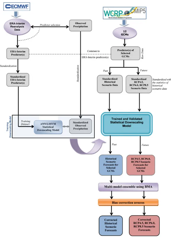
The results of the ANN model show that NS co-efficients in the basin range from 0.57 to 0.84 during the testing period. Although the RSR efficiencies for the ANN model in the basin vary from 0.39 to 0.66, the computed PBIAS statistics are between 9.5 and −20.5%. The PBIAS performances of the ANN model for 36 stations are considered as ‘very good’. Moreover, stations mod-elled with ANN show ‘good’ and ‘very good’ performances in terms of RSR and NS, except for five stations. On the other hand, NS and RSR measures computed from the LSSVM are nearly the same as those of the ANN model. In this sense, the LSSVM also provides ‘good’ and ‘very good’ modelling performances
except for two stations (Fakilli and Ucpinar stations), whereas the PBIAS values for the LSSVM point out ‘very good’ perfor-mance at 36 stations. The perforperfor-mance ratings are available at Moriasi et al. (2007).
During the training and testing of the models, both the ANN and LSSVM gave quite similar results in terms of the perfor-mance indices. Although the two models produced satisfactory results in general, it turned out that slightly better results were obtained with some stations using one of the models rather than the other. According to overall performance criteria during the testing period for each station, it was decided which downscaling model would be used in the stage of downscaling GCM outputs to station scale (see last column in Table 4).
Although the results achieved from the two models showed a good/very good consistency in precipitation predictions at nearly all stations, the capability for extreme value estimation of employed models was found to be restricted at some stations. In the literature, it has been emphasized that this scenario is quite possible because the statistical models may not explain the entire variance of the modelled predictand (Tripathi et al., 2006).
3.2. Downscaling outputs of 12 GCMs to precipitation and
multi-GCM ensemble application
In the previous section, a convenient statistical downscaling model that had a better performance than the other one was sought in order to downscale reliably the raw RCP outputs of used GCMs to precipitation at 39 stations. After the model con-struction for each station, values of pr for individual grids were arranged for the GCMs of the historical scenario and for RCP4.5, RCP6.0, and RCP8.5 future scenarios. According to the down-scaling scheme introduced in Figure 3, after preparing interpo-lated data for each GCM, which are a combination of the values of the nearest grids covering the Gediz Basin (given in the last column of Table 2) and those of neighbouring grids, the RCP datasets were standardized with the historical scenario statistics of the corresponding GCM. These standardized series were con-sidered as the input vector for the selected statistical downscaling models calibrated through the reanalysis variables compiled from eight ERA-Interim grids. Thus, for each GCM, standardized val-ues representing the historical and future scenarios were made
Figure 3. Proposed downscaling strategy applied in the study.
for all meteorological stations. Following the simulation process by trained downscaling model, the obtained standardized values were turned into precipitation unit (in millimetre).
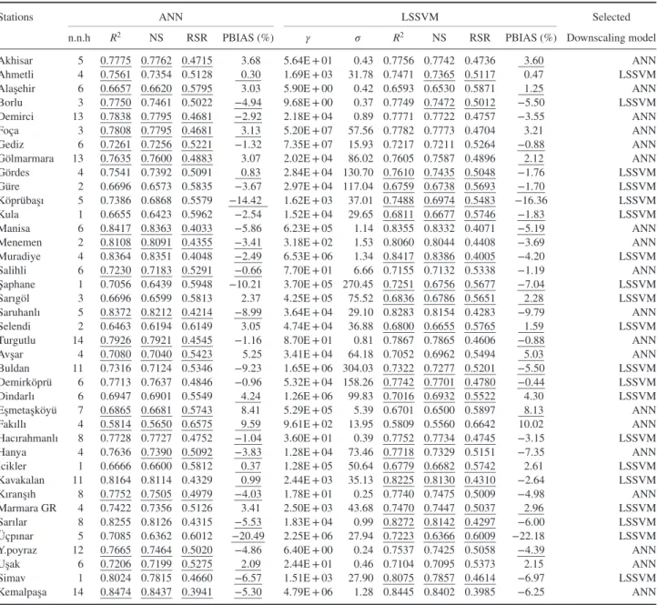
The statistically downscaled precipitation series of 12 GCMs at meteorological station scales were inspected through the box plot graphs under different scenarios. It was seen from the graphs that some descriptive statistics, especially the medians, interquartile ranges and upper whiskers in RCPs, varied relatively from one GCM to another (Figure 5 (a)–(d) for an example at Simav station).
In the literature, there are several inspirational studies focus-ing on the uncertainties originatfocus-ing from the differences between
forecasts obtained from different GCMs (Dibike et al., 2007; Mujumdar and Ghosh, 2008; Okkan and Inan, 2015a). It is apparent that no single GCM is superior to other GCMs for all kinds of downscaling work and under all climatic circumstances. In this respect, the multi-GCM ensemble procedure operating with a group of comparable GCM simulations has been sug-gested by some researchers to deliver more accurate projec-tions (Knutti et al., 2010; Chong-hai and Ying, 2012; Okkan and Inan, 2015a). An ensemble strategy used in hydrological mod-elling studies may also help to improve the uncertainty estima-tion (Duan et al., 2007). A comprehensive review on multi-GCM ensemble applications in the literature and some frequently used
Table 4. Overall performance measures of the artificial neural network (ANN) and least-squares support vector machine (LSSVM) statistical downscaling models for the testing period.
Stations ANN LSSVM Selected
n.n.h R2 NS RSR PBIAS (%) 𝛾 𝜎 R2 NS RSR PBIAS (%) Downscaling model
Akhisar 5 0.7775 0.7762 0.4715 3.68 5.64E + 01 0.43 0.7756 0.7742 0.4736 3.60 ANN Ahmetli 4 0.7561 0.7354 0.5128 0.30 1.69E + 03 31.78 0.7471 0.7365 0.5117 0.47 LSSVM Ala¸sehir 6 0.6657 0.6620 0.5795 3.03 5.90E + 00 0.42 0.6593 0.6530 0.5871 1.25 ANN Borlu 3 0.7750 0.7461 0.5022 −4.94 9.68E + 00 0.37 0.7749 0.7472 0.5012 −5.50 LSSVM Demirci 13 0.7838 0.7795 0.4681 −2.92 2.18E + 04 0.89 0.7771 0.7722 0.4757 −3.55 ANN
Foça 3 0.7808 0.7795 0.4681 3.13 5.20E + 07 57.56 0.7782 0.7773 0.4704 3.21 ANN
Gediz 6 0.7261 0.7256 0.5221 −1.32 7.35E + 07 15.93 0.7217 0.7211 0.5264 −0.88 ANN Gölmarmara 13 0.7635 0.7600 0.4883 3.07 2.02E + 04 86.02 0.7605 0.7587 0.4896 2.12 ANN Gördes 4 0.7541 0.7392 0.5091 0.83 2.84E + 04 130.70 0.7610 0.7435 0.5048 −1.76 LSSVM Güre 2 0.6696 0.6573 0.5835 −3.67 2.97E + 04 117.04 0.6759 0.6738 0.5693 −1.70 LSSVM Köprüba¸sı 5 0.7386 0.6868 0.5579 −14.42 1.62E + 03 37.01 0.7488 0.6974 0.5483 −16.36 LSSVM Kula 1 0.6655 0.6423 0.5962 −2.54 1.52E + 04 29.65 0.6811 0.6677 0.5746 −1.83 LSSVM Manisa 6 0.8417 0.8363 0.4033 −5.86 6.23E + 05 1.14 0.8355 0.8332 0.4071 −5.19 ANN Menemen 2 0.8108 0.8091 0.4355 −3.41 3.18E + 02 1.53 0.8060 0.8044 0.4408 −3.69 ANN Muradiye 4 0.8364 0.8351 0.4048 −2.49 6.53E + 06 1.34 0.8417 0.8386 0.4005 −4.20 LSSVM Salihli 6 0.7230 0.7183 0.5291 −0.66 7.70E + 01 6.66 0.7155 0.7132 0.5338 −1.19 ANN ¸Saphane 1 0.7056 0.6439 0.5948 −10.21 3.70E + 05 270.45 0.7251 0.6756 0.5677 −7.04 LSSVM Sarıgöl 3 0.6696 0.6599 0.5813 2.37 4.25E + 05 75.52 0.6836 0.6786 0.5651 2.28 LSSVM Saruhanlı 5 0.8372 0.8212 0.4214 −8.99 3.64E + 04 29.10 0.8283 0.8154 0.4283 −9.79 ANN Selendi 2 0.6463 0.6194 0.6149 3.05 4.74E + 04 36.88 0.6800 0.6655 0.5765 1.59 LSSVM Turgutlu 14 0.7926 0.7921 0.4545 −1.16 8.70E + 01 0.81 0.7867 0.7865 0.4606 −0.88 ANN Av¸sar 4 0.7080 0.7040 0.5423 5.25 3.41E + 04 64.18 0.7052 0.6962 0.5494 5.03 ANN Buldan 11 0.7316 0.7124 0.5346 −9.23 1.65E + 06 304.03 0.7322 0.7277 0.5201 −5.50 LSSVM Demirköprü 6 0.7713 0.7637 0.4846 −0.96 5.32E + 04 158.26 0.7742 0.7701 0.4780 −0.44 LSSVM Dindarlı 6 0.6947 0.6901 0.5549 4.24 1.26E + 06 99.83 0.7016 0.6932 0.5522 4.30 LSSVM E¸smeta¸sköyü 7 0.6865 0.6681 0.5743 8.41 5.29E + 05 5.39 0.6701 0.6500 0.5897 8.13 ANN Fakıllı 4 0.5814 0.5650 0.6575 9.59 9.61E + 02 13.95 0.5809 0.5560 0.6642 10.02 ANN Hacırahmanlı 8 0.7728 0.7727 0.4752 −1.04 3.60E + 01 0.39 0.7752 0.7734 0.4745 −3.15 LSSVM Hanya 4 0.7636 0.7390 0.5092 −3.83 1.28E + 04 73.46 0.7718 0.7329 0.5151 −7.35 ANN ˙Icikler 1 0.6666 0.6600 0.5812 0.37 1.28E + 05 50.64 0.6779 0.6682 0.5742 2.61 LSSVM Kavakalan 11 0.8164 0.8114 0.4329 0.99 2.44E + 03 35.13 0.8225 0.8130 0.4310 −2.64 LSSVM Kıran¸sıh 8 0.7752 0.7505 0.4979 −4.03 1.78E + 01 0.25 0.7740 0.7475 0.5009 −4.98 ANN Marmara GR 4 0.7422 0.7356 0.5126 3.41 2.50E + 03 43.68 0.7470 0.7447 0.5037 2.96 LSSVM Sarılar 8 0.8255 0.8126 0.4315 −5.53 1.83E + 04 0.99 0.8272 0.8142 0.4297 −6.00 LSSVM Üçpınar 5 0.7085 0.6362 0.6012 −20.49 2.25E + 06 27.94 0.7223 0.6366 0.6009 −22.18 LSSVM Y.poyraz 12 0.7665 0.7464 0.5020 −4.86 6.40E + 00 0.24 0.7537 0.7425 0.5058 −4.39 ANN
U¸sak 6 0.7206 0.7199 0.5275 2.09 2.44E + 01 0.46 0.7104 0.7095 0.5373 2.15 ANN
Simav 1 0.8024 0.7815 0.4660 −6.57 1.51E + 03 27.90 0.8075 0.7857 0.4614 −6.97 LSSVM Kemalpa¸sa 14 0.8474 0.8437 0.3941 −5.30 4.79E + 06 1.28 0.8445 0.8402 0.3985 −6.25 ANN The underlined values in table represent the optimal results.
methods was discussed at the ‘IPCC Expert Meeting on Assess-ing and CombinAssess-ing Multi Model Climate Projections’ by Knutti et al. (2010). Their work provided useful practical advice for using multi-GCM ensembles in climate projections which should be essential for impact-adaptation exercises. In this regard, crite-ria for modelling quality and performance indices, and weighting of employed models were discussed.
Concerning the recommendations of Knutti et al. (2010), the weighted multi-GCM mean approach was preferred, which is an average across all forecasts from multi-GCM simulations, that does not treat the used GCMs equally. In this approach, the weights can be derived from some measures assessing GCM capability in simulating the observed climate conditions (Knutti et al., 2010). The ensemble procedure for this study was per-formed with the Bayesian Model Averaging (BMA) method. This is a statistical scheme designed to obtain probabilistic forecasts with greater ability and reliability than the forecasts obtained by any single model. In some studies, BMA was shown to yield convenient results when it was compared with other ensemble
techniques (Raftery et al., 2005). BMA has been used formerly in hydro-meteorological applications. For example, Raftery et al. (2005) used BMA in order to calibrate forecast ensembles in numerical weather modelling. To the best of our knowledge, a multi-GCM ensemble exercise focusing on the BMA scheme has not been found in the downscaling literature. The BMA method is given concisely as follows.
Consider a quantity y to be the modelled variable, D = [yobs,1,
yobs,2, … , yobs,T] to be the observed data with data size T, and
fk forecasts obtained from the K-model (K = 12 for this study),
where the a posteriori distribution of y is represented as the
conditional probability pk(y|fk, D).
Referencing the total probability law, the probabilistic forecast of BMA is defined as the probability density function shown in Equation ((1): p ( y| D) = K ∑ k=1 p(fk||D)· pk ( y ||fk, D ) (1)
(a) (b) y = 0.8635x + 5.9742 R2 = 0.8640 0 50 100 150 200 250 300 350 400 0 50 100 150 200 250 300 350 400 ANN Akhisar Observed Training 0 50 100 150 200 250 300 350 400 1980 1981 1982 1983 1984 1985 1986 1987 1988 1989 1990 1991 1992 1993 1994 1995 1996 1997 1998 1999 2000 2001 2002 2003 2004 2005 Precipitarion (mm/ month) Akhisar Observed ANN y = 0.7721x + 9.4077 R2 = 0.7775 0 50 100 150 200 250 0 50 100 150 200 250 ANN Akhisar Observed Testing y = 0.8578x + 6.2088 R2 = 0.8655 0 50 100 150 200 250 300 350 400 0 50 100 150 200 250 300 350 400 LSSVM Akhisar Observed Training 0 50 100 150 200 250 300 350 400 1980 1981 1982 1983 1984 1985 1986 1987 1988 1989 1990 1991 1992 1993 1994 1995 1996 1997 1998 1999 2000 2001 2002 2003 2004 2005 Precipitation (mm/month) Akhisar Observed LSSVM y = 0.7660x + 9.7530 R2 = 0.7756 0 50 100 150 200 250 0 50 100 150 200 250 LSSVM Akhisar Observed Testing Training Testing Training Testing
0 50 100 150 200 250 300 (a) (c) (d) (b) Observed BCC-CSM1.1 CCSM4 CESM1(CAM5) Csiro-Mk3.6 GFDL-CM3 GFDL-ESM2M GISS-E2-H GISS-E2-R
HADGEM2-ES IPSL-CM5A-LR MIROC-ESM MRI-CGCM3
Precipitation (mm) Historical (1980–2005) 0 50 100 150 200 250 300 BCC-CSM1.1 CCSM4 CESM1(CAM5) Csiro-Mk3.6 GFDL-CM3 GFDL-ESM2M GISS-E2-H GISS-E2-R
HADGEM2-ES IPSL-CM5A-LR MIROC-ESM MRI-CGCM3
Precipitation (mm) RCP4.5 (2015–2050) 0 50 100 150 200 250 300 BCC-CSM1.1 CCSM4 CESM1(CAM5) Csiro-Mk3.6 GFDL-CM3 GFDL-ESM2M GISS-E2-H GISS-E2-R
HADGEM2-ES IPSL-CM5A-LR MIROC-ESM MRI-CGCM3
Precipitation (mm) RCP6.0 (2015–2050) 0 50 100 150 200 250 300 BCC-CSM1.1 CCSM4 CESM1(CAM5) Csiro-Mk3.6 GFDL-CM3 GFDL-ESM2M GISS-E2-H GISS-E2-R
HADGEM2-ES IPSL-CM5A-LR MIROC-ESM MRI-CGCM3
Precipitation (mm)
RCP8.5 (2015–2050)
Figure 5. Scenario precipitation forecasts obtained from downscaled values of 12 GCMs at Simav station: (a) historical, (b) RCP4.5, (c) RCP6.0 and (d) RCP8.5.
This term also measures how well model forecasts match the observations. To gain a computational convenience in practice,
Gaussian distribution is assumed for pk(y|fk, D), which is also
denoted as g(y|fk,𝜎k2). Assuming that the probability distribution
of precipitation error is non-Gaussian, data are subjected to the Box–Cox transformation before applying BMA. If weights are
defined as wk= p(fk|D), then BMA gives Σwk= 1, where wkare
all positive. The posterior mean of the BMA forecast is defined as shown in Equation ((2): E[y| D]= K ∑ k=1 p(fk||D)· E[pk(y| fk, D)] = K ∑ k=1 wk· fk (2)
To apply the BMA method, weights (wk) and the variance of
model forecast (𝜎k2) must be estimated. The maximization of
a log-likelihood function (Equation ((3)) suggested by Raftery et al. (2005) can be used for this step:
l (𝜃) = l(w1, … , wk; 𝜎1, … , 𝜎k ) = log[ K ∑ k=1 wk· g(y| fk, 𝜎k)] (3)
However, obtaining an analytical solution of 𝜃 by
conven-tional methods is quite difficult. For that reason, Raftery et al. (2005) has recommended an iterative procedure based on the Expectation–Maximization algorithm (E-M). For a detailed description of both the BMA scheme and E-M, readers are referred to Duan et al. (2007).
In order to apply the BMA method for precipitation projection, an ensemble of competing forecasts from 12 GCMs (historical scenario forecasts) was considered. In the study, precipitation forecasts were divided into two periods as wet (from October to March) and dry (from April to September) and then applied the BMA to each period separately. Thus, a different set of BMA weights was obtained for each period. The computed weights for 39 stations were not given due to space limitations. After computing weights for each station during the historical scenario period, downscaled values of 12 GCMs for 3 RCPs were multiplied by these weights and then summed to obtain future scenario results.
3.3. Bias correction
Some studies in the literature have revealed that the results derived from the multi-model mean approach generally outper-form those from single GCMs compared to measured values
(a) (b) (c) Observed Frequency 360 300 240 180 120 60 0 100 80 60 40 20 0 Uncorrected ensemble Frequency 120 100 80 60 40 20 0 25 20 15 10 5 0 Corrected ensemble Frequency 280 240 200 160 120 80 40 0 100 80 60 40 20 0 Mean (mm) 46.450 Min. (mm) 0.001 Mean (mm) Median (mm) 45.890 Min. (mm) 1.910 Median (mm) 46.240 0.000 Median (mm) Cv SD (mm) 28.450 1.129 52.430 Kurtosis Skewness Max. (mm) 4.380 1.760 351.200 Cv SD (mm) Mean (mm) SD (mm) Cv 41.980 0.642 29.460 Kurtosis Skewness Max. (mm)
Min. (mm) Max. (mm) Skewness Kurtosis -0.710 0.410 124.170 31.370 1.116 51.610 3.940 1.760 309.640
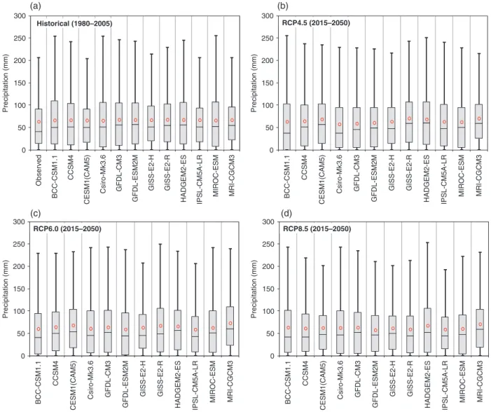
Figure 6. Histogram plots of (a) observed precipitation, (b) uncorrected ensemble forecasts under historical scenario and (c) corrected ensemble
forecasts under historical scenario at Akhisar station.
(Gleckler et al., 2008). However, some biases may be observed in ensemble simulations (Knutti et al., 2010). In this section, fol-lowing the ensemble process based on the BMA scheme given in the previous section, a bias correction technique was used so as to lessen possible biases in ensemble forecasts. It is possible that the forecasts produced from statistical downscaling models may contain some biases due to several reasons attributed to GCM resolution, the predictors, preferred downscaling model type and the climate period. Sachindra et al. (2014) have emphasized that correcting biases is required before use of projections in climate impact studies.
There are various bias correction methods applied to raw GCM outputs and also to the downscaled values. The most frequently used technique is quantile mapping (QM) that can be capable of correcting the statistical moments. In this method, cumula-tive distribution functions (CDFs) of downscaled past scenario results are mapped onto the CDFs of observations. For future climate scenarios, first, corresponding to the downscaled values for future periods, the CDFs are computed from the CDFs relat-ing to the past scenario results. Finally, the corrected values of
a variable for future periods can be extracted from the CDFs of the observations (Sachindra et al., 2014). Lafon et al. (2013) used linear-nonlinear scaling, Gamma distribution-based QM and empirical distribution-based QM (EMQM) in their work. According to their comparisons, EMQM was determined as the best-performing method. EMQM also displayed successful per-formance in a study presented by Themeßl et al. (2011). Ines and Hansen (2006) compared the performances of QM and the multiplicative shift method (MSF) in correcting the bias for precipitation values. They concluded that MSF corrected the long-term monthly mean precipitation. However, this method is unsuccessful for correcting systematic errors in precipitation distribution. Sachindra et al. (2014) presented a comprehensive study involving the usage of equidistant QM (EDQM), monthly bias-correction (MBC) and nested bias-correction (NBC) meth-ods. When considering the performances of three methods, EDQM was preferred for preparing future precipitation projec-tions in their work.
In this study, QM based bias correction strategy was applied. The approach employed, which was formulized by Ghosh and Mujumdar (2008), used CDFs to reduce the biases existing in scenario forecasts. In this bias-correction application, monthly precipitation values at 39 stations, which were obtained from the multi-GCM ensemble, were assessed for the reference period 1980–2005 under the historical scenario. Then, the probability plot correlation co-efficient test revealed that the two-parameter Gamma distribution fitted well at 39 stations. The CDFs per-taining to the observed data and the ensemble forecasts of four scenarios were computed. However, they are not presented due to page number restriction. The yield of the bias correction appli-cation in facilitating the distributional features of the forecasted precipitation values under the historical scenario to be conve-nient with those of observations at Akhisar station can be seen in Figure 6. The computed statistics of precipitation forecasts for the same example are given in Figure 6, also. Although the
arithmetical mean, standard deviation, variation (Cv), median
and maximum value statistics of the observed precipitation at Akhisar station are 46.45 mm, 52.43 mm, 1.129, 28.45 mm and 351.2 mm, respectively, those of precipitation forecasts for the historical scenario before correcting biases were 45.89 mm, 29.46 mm, 0.642, 41.98 mm and 124.17 mm, respectively. After correcting biases, these parameters under the historical scenario were 46.24 mm, 51.61 mm, 1.116, 31.37 mm and 309.6 mm, respectively. These results show that the biases were reduced meaningfully for the Akhisar station example. Similar inferences were found to be acceptable for the other 38 stations as well.
3.4. Hypothesis testing on historical scenario results
In order to have confidence in the climate change scenarios downscaled statistically from GCMs, assurance is required that the downscaled values can represent past climatic conditions closely (Dibike et al., 2007). After bias correction, a method was employed in the study to analyse the confidence levels of both the downscaled results of the 12 GCMs and ensemble simula-tions derived from the BMA scheme, namely hypothesis testing based on the Mann–Whitney U-test, which was suggested by Dibike et al. (2007) also in uncertainty analyses of downscaled precipitation regimes. The formulations of this test were given by Okkan and Inan (2015a).
If the obtained asymptomatic significance values are greater than or equal to 5%, then there is no meaningful difference between observed and forecasted values in terms of the medians. As shown in Table 5 for Akhisar station, the Mann–Whitney
Table 5. Asymptomatic significance values derived from hypothesis testing for Akhisar station.
Climate model Jan. Feb. Mar. Apr. May Jun. Jul. Aug. Sep. Oct. Nov. Dec.
BCC-CSM1.1 (%) 38.97 21.33 36.98 0.75 18.16 27.22 24.52 35.54 1.65 0.27 59.56 19.38 CCSM4 (%) 38.97 18.76 100.00 66.05 16.43 CESM1(CAM5) (%) 16.99 82.62 25.65 2.81 2.56 0.06 8.37 33.66 95.62 34.13 39.99 95.62 0.01 44.76 66.05 98.54 74.18 19.38 63.42 Csiro-Mk3.6 (%) 2.32 9.22 52.18 8.21 11.55 53.38 64.73 6.19 25.65 3.86 85.48 74.18 GFDL-CM3 (%) 38.97 91.26 34.13 7.89 GFDL-ESM2M (%) 13.82 39.99 5.94 11.55 6.19 4.41 0.00 46.41 10.14 18.16 72.80 95.62 95.62 0.07 24.89 82.62 41.02 68.05 54.59 16.43 GISS-E2-H (%) 82.62 55.81 5.24 GISS-E2-R (%) 54.59 18.16 1.16 0.11 94.16 11.98 0.04 76.97 0.11 3.38 HADGEM2-ES (%) 62.12 52.18 67.38 15.34 4.61 0.04 IPSL-CM5A-LR (%) 36.98 20.67 79.78 0.27 74.18 0.00 0.03 1.74 0.12 64.73 70.07 0.00 64.73 7.89 31.86 1.74 21.33 18.16 45.30 43.13 0.01 3.23 13.82 70.07 3.95 5.70 79.78 0.41 71.43 MIROC-ESM (%) 42.07 86.92 21.33 12.42 16.43 13.34 16.71 16.99 24.15 66.71 62.12 5.70 MRI-CGCM3 (%) 13.34 0.51 6.72 10.34 2.01 0.03 0.08 46.97 24.15 0.01 95.62 31.41 ENSEMBLE (%) 91.26 86.92 92.71 85.48 85.48 74.18 25.65 9.95 36.02 98.54 92.71 84.05
The shaded characters in table displays that there is a significant difference between the observation and forecasted values for the median statistics.
Figure 7. Precipitation changes (in %) in relation to the 1980–2005 historical scenario period for (a) RCP4.5, (b) RCP6.0 and (c) RCP8.5
scenarios.
U-test was implemented at the 5% level of significance to exam-ine whether precipitation forecasts in the historical scenario were meaningfully different from observation statistics or not. Accord-ing to analyses, it is interpreted that the corrected ensemble simu-lations are better than those of single GCMs. In other words, the
combined use of the BMA-based ensemble procedure and bias correction approach was able to reproduce the median charac-teristics of monthly precipitation reasonably well. Similar results were obtained for the corrected ensemble simulations at the other 38 stations which were not presented here.
3.5. Foreseen changes in future precipitation
It is hoped that produced forecasts are not only reliable because multi-GCM ensemble application is more consistent than a single GCM usage, but also de-biased after the bias correction procedure. The distributions of precipitation changes are shown in Figure 7 for the considered future period (2015–2050) under three RCP scenarios. In the present study, in order to investigate whether the mean statistics related to produced forecasts under the three RCP scenarios reflecting the future period were statis-tically distinct from those of the historical scenario (1980–2005 climate), a two-sample t-test was operated at the 5% significance level.
The results in Figure 7 reveal that the precipitation over the basin tended to decrease in the future for all three RCP scenarios. However, remarkable decreases were found only in the RCP8.5 results, where the foreseen changes were statistically significant by t-test for nearly all stations. According to the RCP8.5 sce-nario, decreasing precipitation in the western part of the basin and some regions nearest to Golmarmara Lake and Demirkopru Dam and Gordes Dam reservoirs was more obvious than in the northwestern and northeastern parts of the Basin, whereas effec-tive decreases also were found in the southeastern part of the basin, where the decreasing proportion was foreseen as 18.5%.
In order to interpret foreseen changes in precipitation over the whole basin, Thiessen weighted precipitation (TWP) val-ues were obtained from all 39 stations. TWP obtained from the scenario forecasts for the 39 stations for both seasonal and annual periods are given (Figure 8). Although decreases were foreseen in all seasons under RCP8.5, it was much more dis-tinctive in autumn. Moreover, the decreases foreseen in win-ter and autumn will affect annual precipitation regime because the total precipitation measured in winter and autumn repre-sents nearly half of the total precipitation potential of the basin. When the annual mean statistics were considered, 8, 10 and 17% decreases were foreseen related to RCP4.5, RCP6.0, and RCP8.5 scenarios, respectively. Moreover, the box-plot graphs given in Figure 8 show that there will be decreases in the forecasts of third quartiles (high-rainfall), particularly in the RCP8.5 results. When the projected surface air temperature, which is expected
50 100 150 200 250 300 350 400 450 500 Historical RCP4.5 RCP6.0 RCP8.5 Winter precipitation (mm) 0 50 100 150 200 250 300 Historical RCP4.5 RCP6.0 RCP8.5 Spring precipitation (mm) 0 10 20 30 40 50 60 70 80 Historical RCP4.5 RCP6.0 RCP8.5 Summer precipitation (mm) 0 50 100 150 200 250 Historical RCP4.5 RCP6.0 RCP8.5 Autumn precipitation (mm) 200 300 400 500 600 700 800 Historical RCP4.5 RCP6.0 RCP8.5 Annual precipitation (mm) (a) (b) (c) (d) (e)
Figure 8. TWP calculated from the scenario forecasts of 39 stations for (a) winter, (b) spring, (c) summer, (d) autumn and (e) annual periods.
to increase markedly in all three RCP scenarios, is also taken into account, it becomes inevitable that the basin may experience water scarcity problem between the years 2015 and 2050.
4. Conclusions
The analysis of precipitation has a very important role to play in water resource management, such as planning of irriga-tion systems, dam reservoir operairriga-tion, water budget studies and watershed modelling. In this study, projection of monthly precipitation over the Gediz Basin under several Representative Concentration Pathways (RCP) scenarios mentioned in the
IPCC 5thAssessment Report (AR5) was performed by a
mod-elling strategy consisting of artificial neural network (ANN) / least-squares support vector machine (LSSVM) techniques, multi-general circulation model (GCM) ensemble and bias correction.
The statistical downscaling models were calibrated and tested using both observed precipitation and the ERA-Interim reanal-ysis predictor. The performance examination of the downscaled precipitation predictions at 39 stations denoted that the trained models generated consistent results, in contrast to various works in the literature where daily precipitation downscaling was car-ried out (e.g. Dibike et al., 2007). In other words, the good or very good agreement between observed and predicted monthly values
at meteorological stations indicated that the trained models with the set of optimized parameters could be applied to examine the responses of precipitation due to climate changes in the Basin.
Hence, the effectiveness of statistical downscaling models was illustrated through their integration to a historical scenario (1980–2005) and three RCP future scenarios (2015–2050). At this stage, simulations from 12 GCMs, which are available at CMIP5, were considered to obtain projections of precipitation at 39 stations. The eventual precipitation forecasts were produced from a multi-GCM ensemble application based on a Bayesian Model Averaging (BMA) method and bias correction technique. The quantile mapping based-bias correction (QM) approach employed in this study, which uses cumulative distribution func-tions (CDFs), especially for hydrological variables coming from a skewed distribution, was also preferred by other researchers. By using hypothesis testing, the ability of corrected ensemble forecasts to simulate the historical climate in terms of statisti-cal moments was assessed. Sachindra et al. (2014) have empha-sized that quantile mapping is not able to correct the time series explicitly. Otherwise, methods such as monthly bias-correction and nested bias-correction are able to correct some of the statis-tics without disrupting the temporal sequence (Sachindra et al., 2014). Therefore, the QM approach presented herein will be compared with other bias correction methods in a future work in order to ensure the validation of the results derived from this study.
Following the investigation of historical scenario results, the significances of the computed changes for the 2015–2050 future period were examined statistically. According to statistical inves-tigations for different emission scenarios, insignificant decreases are foreseen over the Basin for RCP4.5 and RCP6.0, whereas sig-nificant decreasing trends in precipitation are identified for the RCP8.5 scenario. Considering that the RCP8.5 scenario results can be defined as a pessimistic scenario with comparatively high greenhouse gas emissions, it is foreseen that there will be around 17% decrease in mean areal precipitation over the basin com-pared to the reference climate period.
As is well-known, in downscaling works the possible effects of climatic change on variables operating within the hydro-logical cycle are all related within the uncertainty/reliability frame. It was uttered that uncertainties are related to GCMs, used scenarios, data features, and the used downscaling tech-niques (Mujumdar and Ghosh, 2008; Okkan and Inan, 2015a). In spite of the aforementioned uncertainties, statistical down-scaling techniques will remain the most frequently used tools for researchers to examine the effects of climate change on hydrological processes owing to their computational practical-ity compared to dynamic downscaling (Anandhi et al., 2008). Moreover, the use of 12 GCMs with 3 RCP scenarios, two statis-tical downscaling models trained with optimal predictor selection and an ensemble procedure should serve as inspiration for pre-cipitation projections of other important basins in Turkey and beyond.
Duan et al. (2007) stated that different models may have strengths in capturing different aspects of hydro-meteorological processes. Enough knowledge about the uncertainty relevant to the forecasts derived from single models currently may not be available. However, the uncertainties and structural errors observed in any single model are at insignificant orders for ensemble applications. In this regard, focusing on both Bayesian model averaging and bias correction methods for this study resulted in robust climate modelling and a reliable projection.
The inferences obtained from this work point out that the developed strategy is a conceivable option for downscaling
precipitation to a basin scale. Hence, a similar study concerning surface air temperature projection for the same basin will be per-formed in a future study. However, it is proposed that dynamical downscaling tools (e.g. REGCM4, PRECIS) and other statistical models used in the literature can be used to check for inter-model robustness of the downscaled forecasts for the study area. A com-prehensive research effort in this direction is also planned.
The results presented herein will also be assessed in future work through the integration of rainfall–runoff models. Follow-ing buildFollow-ing a rainfall–runoff model for the sub-basins in the Basin, the downscaled precipitation and temperature values can be converted into streamflows by operating a calibrated hydro-logical model.
Acknowledgements
The research leading to this study is funded by the Scientific and Technological Research Council of Turkey (TUBITAK) under Grant No. 114Y716. The authors would like to thank the Turkish State Meteorological Service (MGM) and General Directorate of State Hydraulic Works (DSI) for their help with data collection. The authors also wish to thank the editor and the two anonymous reviewers for their constructive comments that improved the quality of this paper.
References
Anandhi A, Srinivas VV, Nanjundiah RS, Nagesh Kumar D. 2008. Downscaling precipitation to river basin in India for IPCC SRES scenarios using support vector machine. Int. J. Climatol. 28: 401–420. Bürger G, Murdock TQ, Werner AT, Sobie SR, Cannon AJ. 2012. Down-scaling extremes-an intercomparison of multiple statistical methods for present climate. J. Clim. 25: 4366–4388.
Chen H, Guo J, Xiong W, Guo S, Xu C-Y. 2010. Downscaling GCMs using the Smooth Support Vector Machine method to predict daily precipitation in the Hanjiang Basin. Adv. Atmos. Sci. 27: 274–284. Chong-hai X, Ying X. 2012. The projection of temperature and
precip-itation over China under RCP Scenarios using a CMIP5 multi-model ensemble. Atmos. Ocean. Sci. Lett. 5: 527–533.
Dibike YB, Gachon P, St-Hilaire A, Ouarda TBMJ, Nguyen VTV. 2007. Uncertainty analysis of statistically downscaled temperature and precipitation regimes in Northern Canada. Theor. Appl. Climatol. 91: 149–170.
Duan Q, Ajami N, Gao X, Sorooshian S. 2007. Multi-model ensemble hydrologic prediction using Bayesian model averaging. Adv. Water Resour. 30: 1371–1386.
Fistikoglu O, Okkan U. 2011. Statistical downscaling of monthly pre-cipitation using NCEP/NCAR reanalysis data for tahtali river basin in Turkey. J. Hydrol. Eng. 16: 157–164.
Fowler HJ, Blenkinsop S, Tebaldi C. 2007. Linking climate change mod-elling to impacts studies: recent advances in downscaling techniques for hydrological modelling. Int. J. Climatol. 27: 1547–1578. Ghosh S, Mujumdar PP. 2008. Statistical downscaling of GCM
sim-ulations to streamflow using relevance vector machine. Adv. Water Resour. 31: 132–146.
Gleckler P, Taylor K, Doutriaux C. 2008. Performance metrics for climate models. J. Geophys. Res. 113: D06104.
Goyal MK, Ojha CSP. 2012. Downscaling of surface temperature for lake catchment in an arid region in India using linear multiple regres-sion and neural networks. Int. J. Climatol. 32: 552–566.
Haas R, Pinto JG. 2012. A combined statistical and dynamical approach for downscaling large-scale footprints of European windstorms. Geo-phys. Res. Lett. 39: L23804.
Hagan MT, Menhaj MB. 1994. Training feedforward networks with the Marquardt algorithm. IEEE. Trans. Neural. Netw. 5: 989–993. Hessami M, Gachon P, Ouarda TBMJ, St-Hilaire A. 2008. Automated
regression-based statistical downscaling tool. Environ. Modell. Softw. 23: 813–834.
Ines AVM, Hansen JW. 2006. Bias correction of daily GCM rainfall for crop simulation studies. Agric. For. Meteorol. 138: 44–53.
Ji Z, Kang S. 2013. Double-nested dynamical downscaling experiments over the Tibetan Plateau and Their Projection of climate change under Two RCP Scenarios. J. Atmos. Sci. 70: 1278–1290.
Kim J, Choi J, Choi C, Park S. 2013. Impacts of changes in climate and land use/land cover under IPCC RCP scenarios on streamflow in the Hoeya River Basin. Korea. Sci. Total. Environ. 452–453: 181–195. Knutti R, Abramowitz G, Collins M, Eyring V, Gleckler PJ, Hewitson B
et al. 2010. Good practice guidance paper on assessing and combining multi model climate projections. IPCC Expert Meeting on Assessing and Combining Multi Model Climate Projections: Boulder, CO; 15pp. Lafon T, Dadson S, Buys G, Prudhomme C. 2013. Bias correction of daily precipitation simulated by a regional climate model: a compari-son of methods. Int. J. Climatol. 33: 1367–1381.
Lee JW, Hong SY, Chang EC, Suh MS, Kang HS. 2014. Assessment of future climate change over East Asia due to the RCP scenarios downscaled by GRIMs-RMP. Clim. Dyn. 42: 733–747.
Leung LR, Mearns LO, Giorgi F, Wilby RL. 2003. Regional climate research: needs and opportunities. Bull. Am. Meteorol. Soc. 84: 89–95. Meinshausen M, Smith SJ, Calvin K, Daniel JS, Kainuma MLT, Lamar-que J, et al. 2011. The RCP greenhouse gas concentrations and their extensions from 1765 to 2300. Clim. Change 109: 213–241. Moriasi DN, Arnold JG, Van Liew MW, Bingner RL, Harmel RD, Veith
TL. 2007. Model evaluation guidelines for systematic quantification of accuraccy in watershed simulations. Trans. Asabe. 50: 885–900. Moss RH, Edmonds JA, Hibbard KA, Manning MR, Rose SK, van
Vuuren DP, et al. 2010. The next generation of scenarios for climate change research and assessment. Nature 463: 747–756.
Mujumdar PP, Ghosh S. 2008. Modeling GCM and scenario uncertainty using a possibilistic approach: application to the Mahanadi River. India. Water. Resour. Res. 44: W06407, DOI: 10.1029/2007WR006137.
Okkan U. 2015. Assessing the effects of climate change on monthly precipitation: proposing of a downscaling strategy through a case study in Turkey. KSCE J. Civ. Eng. 19: 1150–1156.
Okkan U, Fistikoglu O. 2014. Evaluating climate change effects on runoff by statistical downscaling and hydrological model GR2M. Theor. Appl. Climatol. 117: 343–361.
Okkan U, Inan G. 2015a. Statistical downscaling of monthly reservoir inflows for Kemer watershed in Turkey: use of machine learning methods , multiple GCMs and emission scenarios. Int. J. Climatol. 35: 3274–3295.
Okkan U, Inan G. 2015b. Bayesian learning and relevance vector machines approach for downscaling of monthly precipitation. J. Hydrol. Eng. 20, DOI: 10.1061/(ASCE)HE.1943-5584.0001024. Raftery AE, Gneiting T, Balabdaoui F, Polakowski M. 2005. Using
bayesian model averaging to calibrate forecast ensembles. Mon. Weather Rev. 133: 1155–1174.
Riahi K, Rao S, Krey V, Cho C, Chirkov V, Fischer G, et al. 2011. RCP 8.5-A scenario of comparatively high greenhouse gas emissions. Clim. Change. 109: 33–57.
Sachindra DA, Huang F, Barton A, Perera BJC. 2013. Least square support vector and multi-linear regression for statistically downscaling general circulation model outputs to catchment streamflows. Int. J. Climatol. 1106: 1087–1106.
Sachindra DA, Huang F, Barton A, Perera BJC. 2014. Statistical down-scaling of general circulation model outputs to precipitation-part 2: bias-correction and future projections. Int. J. Climatol. 34: 3282–3303.
Salathé EP. 2003. Comparison of various precipitation downscaling methods for the simulation of streamflow in a rainshadow river basin. Int. J. Climatol. 23: 887–901.
Schmidli J, Frei C, Vidale PL. 2006. Downscaling from GCM precipita-tion: a benchmark for dynamical and statistical downscaling methods. Int. J. Climatol. 26: 679–689.
Semenov MA. 2008. Simulation of extreme weather events by a stochas-tic weather generator. Clim. Res. 35: 203–212.
Singh V, Goyal MK. 2016. Analysis and trends of precipitation lapse rate and extreme indices over north Sikkim eastern Himalayas under CMIP5ESM-2 M RCPs experiments. Atmos. Res. 167: 34–60.
Suykens JAK. 2001. Nonlinear modelling and support vector machines. IMTC 2001. Proceedings of the 18th IEEE Instrumentation Measure-ment Technology Conference Rediscovering MeasureMeasure-ment in the Age of Informatics (Cat. No.01CH 37188), 21–23 May 2001, Budapest, Hungary.
Tatli H, Dalfes N, Mente¸s S. 2004. A statistical downscaling method for monthly total precipitation over Turkey. Int. J. Climatol. 24: 161–180.
Themeßl M, Gobiet A, Leuprecht A. 2011. Empirical-statistical down-scaling and error correction of daily precipitation from regional cli-mate models. Int. J. Climatol. 31: 1530–1544.
Tripathi S, Srinivas VV, Nanjundiah RS. 2006. Downscaling of pre-cipitation for climate change scenarios: a support vector machine approach. J. Hydrol. 330: 621–640.
Vu MT, Aribarg T, Supratid S, Raghavan SV, Liong S-Y. 2015. Statistical downscaling rainfall using artificial neural network: significantly wetter Bangkok? Theor. Appl. Climatol., DOI: 10.1007/s00704-015-1580-1.
Wilby R, Dawson C, Barrow E. 2002. A decision support tool for the assessment of regional climate change impacts. Environ. Model. Softw. 17: 145–157.
Wilby RL, Hassan H, Hanaki K. 1998. Statistical downscaling of hydrometeorological variables using general circulation model output. J. Hydrol. 205: 1–19.
Wilby RL, Wigley TML. 1997. Downscaling general circulation model output: a review of methods and limitations. Prog. Phys. Geogr. 21: 530–548.
Xoplaki E, González-Rouco JF, Luterbacher J, Wanner H. 2004. Wet sea-son Mediterranean precipitation variability: influence of large-scale dynamics and trends. Clim. Dyn. 23: 63–78.