InfoTrad: An R package for estimating the
probability of informed trading
by Duygu Çelik and Murat Tiniç
Abstract The purpose of this paper is to introduce the R package InfoTrad for estimating the proba-bility of informed trading (PIN) initially proposed byEasley et al.(1996). PIN is a popular information asymmetry measure that proxies the proportion of informed traders in the market. This study provides a short survey on alternative estimation techniques for the PIN. There are many problems documented in the existing literature in estimating PIN. InfoTrad package aims to address two problems. First, the sequential trading structure proposed byEasley et al.(1996) and later extended byEasley et al. (2002) is prone to sample selection bias for stocks with large trading volumes, due to floating point exception. This problem is solved by different factorizations provided byEasley et al.(2010) (EHO factorization) andLin and Ke(2011) (LK factorization). Second, the estimates are prone to bias due to boundary solutions. A grid-search algorithm (YZ algorithm) is proposed byYan and Zhang(2012) to overcome the bias introduced due to boundary estimates. In recent years, clustering algorithms have become popular due to their flexibility in quickly handling large data sets.Gan et al.(2015) propose an algorithm (GAN algorithm) to estimate PIN using hierarchical agglomerative clustering which is later extended byErsan and Alici(2016) (EA algorithm). The package InfoTrad offers LK and EHO factorizations given an input matrix and initial parameter vector. In addition, these factorizations can be used to estimate PIN through YZ algorithm, GAN algorithm and EA algorithm.
Introduction
The main aim of this paper is to present theInfoTradpackage that estimates the probability of informed trading (PIN) initially proposed byEasley et al.(1996). PIN is one of the primary measures of proxy information asymmetry in the market. The structural model is driven from maximum likelihood estimation (MLE). Wide range of studies use PIN to answer questions in different fields of finance1.
Although it is a heavily used measure in the finance literature, the development of applications that calculate PIN are quite slow. An initial attempt for R community is made byZagaglia(2012).FinAsym
package ofZagaglia(2012) and thePINpackage ofZagaglia(2013) provide the trade classification algorithm ofLee and Ready(1991) which is an important tool for studies that use the TAQ database. Both packages also provide PIN estimates through pin_likelihood() functions. However, those estimates are prone to bias due to misspecification and other limitations. InfoTrad package aims to overcome such limitations and provide users with a wide range of options when estimating PIN.
Due to the popularity of the measure, problems in estimating PIN recently gained attention in the finance literature.Easley et al.(2010) indicate that for stocks with a large trading volume, it is not possible to estimate PIN due to floating-point-exception (FPE). Two different numerical factorizations are provided byEasley et al.(2010) andLin and Ke(2011) to overcome the bias created due to FPE.
In addition, boundary solutions in estimating PIN are also shown to create bias in empirical studies. Yan and Zhang(2012) show that, independent of the type of factorization, the likelihood function can stuck at local optimum and provide biased PIN estimates. They propose an algorithm (YZ algorithm) that spans the parameter space by using 125 different initial values for the MLE problem and obtain the PIN estimate that gives the highest likelihood value with non-boundary solutions. Although YZ algorithm provides estimates with higher likelihood and guarantees obtain non-boundary solutions, the iterative structure makes this algorithm time-consuming especially for studies that use large datasets.
Considering the fact that recent studies that estimate PIN use large datasets, the effectiveness of the YZ algorithm is questioned. In recent years, clustering algorithms have become popular due to their efficiency in processing large sets of data.Gan et al.(2015) propose an algorithm that use hierarchical agglomerative clustering to estimate PIN.Ersan and Alici(2016) later extends this framework.
FPE and boundary solutions are not the only problems of PIN model.Duarte and Young(2009) indicate that the structural model ofEasley et al.(1996) enforces a negative contemporaneous covari-ance between intraday buy and sell orders, which is contrary to the empirical evidence for symmetric order shocks. In addition,they show that the PIN model fails to capture the volatility of buy and sell orders,through simulations. Moreover,Duarte and Young(2009) adjust PIN to take into account the liquidity impact and show that liquidity is more prominent on stock returns compared to information
1For instance, analyst coverage (Easley et al.,1998), stock splits (Easley et al.,2001), initial public offerings (Ellul
and Pagano,2006), credit ratings (Odders-White and Ready,2006), M&A announcements (Aktas et al.,2007) and asset returns [(Easley et al.,2002),(Easley et al.,2010)] among others.
asymmetry. Finally, it is important to note that PIN does not consider any strategic behaviour of investors such as order splitting. Order splitting can be more evident when a stock is jointly trading on multiple venues (Menkveld,2008). Even for a stock that is traded on a single market, an informed investor may want to split her order in order avoid revealing her private information too quickly (Foucault et al.,2013). PIN model, by construction, fails to attach multiple small orders to a single informed investor.
This paper introduces and discusses the R (R Core Team,2016) InfoTrad package for estimating PIN. InfoTrad provides users with the necessary methods to solely adress the problems of FPE and boundary solutions. The package contains the likelihood factorizations of EHO and LK as separate functions (EHO() and LK(), respectively) which provide likelihood specifications to avoid FPE. In addition, through YZ(), GAN() and EA() functions, PIN estimates can be obtained using the grid-search algorithm ofYan and Zhang(2012) and clustering algorithms ofGan et al.(2015) andErsan and Alici (2016). For all of the algorithms, likelihood specification can be set to EHO or LK.
The paper is organized as follows; Section2.2provides a brief description of PIN. Specifically, section2.2.1discusses the problem of FPE and the alternative factorizations EHO and LK. Section2.2.2 reviews the problem of boundary solutions and the YZ algorithm. Section2.2.3describes the clustering algorithms ofGan et al.(2015) andErsan and Alici(2016). Section2.3introduces the package InfoTrad along with examples. Section2.4evaluates the performance of each method through simulations. Section2.5provides concluding remarks.
PIN Model
The structural model ofEasley et al.(1996) andEasley et al.(2002) consists of three types of agents; informed traders, uninformed traders and market makers. On a trading day t, one risky asset is continuously traded. Market maker sets the price for a given stock by observing the buy orders(Bt)
and sell orders(St). For that stock, an information event is assumed to follow a Bernoulli distribution
with success probability α. This event reveals either a high or a low signal for the stock value. The event is assumed to provide a low signal with probability δ. When informed traders observe a high (low) signal, they are assumed to place buy (sell) orders at a rate of µ. Uninformed traders are assumed to place orders, independent of the information event and the signal. They arrive to market to place a buy (sell) order at a rate of eb(es). Orders of both informed and uninformed investors are assumed to
follow independent Poisson processes.
The joint probability distribution with respect to the parameter vectorΘ≡ {α, δ, µ, eb, es}and the
number of buys and sells(Bt, St), is specified by
f(Bt, St|Θ) ≡αδex p(−eb) ebBt Bt!exp [−(es+µ)](es+µ) St St! +α(1−δ)exp[−(eb+µ)](eb+µ) Bt Bt! exp(−es)e St s St! +(1−α)exp(−eb) eBbt Bt! exp(−es)e St s St! (1)
The estimates of arrival rates ( ˆµ, ˆesand ˆeb), along with estimates of the probabilities (ˆα and ˆδ) can
be obtained by maximizing the joint log-likelihood function given the order input matrix(Bt, St)over
T trading days. The non-linear objective function of this problem can be written as; L(Θ|T) ≡ T
∑
t=1 L(Θ|(Bt, St)) = T∑
t=1 log[f(Bt, St|Θ)] (2)The maximization problem is subject to the boundary constraints α, δ∈ [0, 1]and µ, eb, es∈ [0,∞)2.
The PIN estimate is then given by;
d
PI N= ˆα ˆµ
ˆα ˆµ+eˆb+eˆs
(3)
2Both PIN package ofZagaglia(2013) and FinAsym package of Zagaglia(2012) fail to acknowledge the
boundary constraints on arrival rates µ, eb, es. Similar to event probabilities, they restrict these parameters to[0, 1]
which forces the estimates for the arrival of informed and uninformed traders on a given day to take values at most one. This creates significant bias in PIN estimates.
Floating-Point Exception
PIN estimates are prone to selection bias, especially for stocks for which the number of buy and sell orders are large3.Lin and Ke(2011) show that the increase in the number of buy and sell orders for a given stock, significantly shrinks the feasible solution set for the maximization of the log likelihood function in equation (2). To maximize the non-linear function (1), the optimization software introduces initial values for the parameters inΘ. The numerical optimization method is applied after those initial parameters are introduced. Therefore, for large enough Btand Stwhose factorials cannot be calculated
by mainstream computers (i.e. FPE), the optimal value for equation (2) becomes undefined. The FPE problem is therefore, more pronounced in active stocks.
To avoid the bias created due to FPE, one factorization of the equation (2) is provided byEasley et al.(2010) as LEHO(Θ|T) ≡∑t=1T LEHO(Θ|Bt, St)where
LEHO(Θ|Bt, St) =log[αδex p(−µ)xBbt−Mtx−Ms t+α(1−δ)exp(−µ)x−Mb txSst−Mt+ (1−α)xBbt−MtxSst−Mt]
+Btlog(eb+µ) +Stlog(es+µ) − (eb+es) +Mt[log(xb) +log(xs)] −log(St!Bt!),
(4) where Mt=min(Bt, St) +max(Bt, St)/2, xb=eb/(µ+eb)and xs=es/(µ+es).
Lin and Ke(2011) introduce another algebraically equivalent factorization of the equation (2), LLK(Θ|T) ≡∑Tt=1LLK(Θ|Bt, St)where
LLK(Θ|Bt, St) =log[αδex p(e1t−emaxt) +α(1−δ)exp(e2t−emaxt) + (1−α)exp(e3t−emaxt)]
+Btlog(eb+µ) +Stlog(es+µ) − (eb+es) +emaxt−log(St!Bt!),
(5) where e1t= −µ−Btlog(1+µ/eb), e2t= −µ−Stlog(1+µ/es), e3t= −Btlog(1+µ/eb) −Stlog(1+
µ/es)and emaxt=max(e1t, e2t, e3t). The last term log(St!Bt!)is constant with respect to the parameter
vectorΘ, and is, therefore, dropped in the MLE for both factorizations.
Boundary Solutions
Another source of bias in estimating PIN arises from boundary solutions. Yan and Zhang(2012) indicate that in calculating PIN, parameter estimates ˆα and ˆδ usually fall onto the boundaries of the parameter space, that is, they are equal to zero or one. PIN estimate presented in equation (3) is directly related to the estimate of ˆα. Letting ˆα equal to zero will make sure that PIN is zero as well. This can create a sample selection bias in portfolio formation, especially for quarterly estimations4.Yan and Zhang(2012) show that;
E(B) =α(1−δ)µ+eb (6)
E(S) =αδµ+es (7)
Then, they propose the following algorithm to overcome the bias created due to boundary solutions. Let(α0, δ0, e0b, e0s, µ0)be the initial parameter function to be placed in the non-linear program presented in equation (4). In addition, let ¯B and ¯S be the average number of buy and sell orders.
α0=αi, δ0=δj, e0b=γkB,¯ µ0= ¯ B−e0b α0(1−δ0) and e 0 s=S¯−α0δ0µ0 (8)
where αi, δj, γk∈ {0.1, 0.3, 0.5, 0.7, 0.9}. This will yield 125 different PIN estimates along with their
likelihood values. In line withYan and Zhang(2012), we drop any initial parameter vector having negative values for e0
s. In addition, followingErsan and Alici(2016), we also drop any initial parameter
vector with µ0 > max(Bt, St). Yan and Zhang(2012) then select the estimate with non-boundary
parameters yielding highest likelihood value. This method, by construction, spans the parameter space and tries to avoid local optima and provides non-boundary estimates for α.
3For example,Zagaglia(2012) provides a sample data to calculate PIN. In sample data the maximum trade
number is 19. If you multiply each observation in the sample data by 10, thepin_likelihood()function of FinAsympackage fails to provide results with the sample initial parameter vector.
4For quarterly estimations of PIN, one can be sure that there is at least one information event, earnings
Clustering Approach
In recent years, clustering algorithms are increasingly becoming popular in estimating the probability of informed trading due to efficiency concerns. Gan et al.(2015) andErsan and Alici(2016) use clustering algorithms to estimate PIN.Gan et al.(2015) introduce a method that clusters the data into three groups (good news, bad news, no news) based on the mean absolute difference in order imbalance. Let Xt =Bt−Stbe the order imbalance on day t computed as the difference between
buy orders and sell orders. The clustering is then based on the distance function defined as D(I, J) = |Xi−Xj|, 1≤i, j≤T where i6=j. They use hierarchical agglomerative clustering (HAC) to group
the data elements based on the distance matrix. Specifically, they use hclust() function ofMüllner (2013) in R5. The algorithm sequentially clusters, in a bottom-up fashion, each observation into groups based on Xtand stops when it reaches three clusters. The theoretical framework ofEasley et al.(1996)
indicates that a stock has high (low) Xt on good (bad) days. Therefore, the cluster which has the
highest (lowest) mean Xtis labelled as good (bad) news. The remaining cluster is then labelled as no
news. Once each observation is grouped into their respective clusters (good news, bad news, no news), c ∈ {G, B, N}, the parameter estimates forΘ≡ {α, δ, µ, eb, es}are calculated simply by counting.
Let ωcbe the proportion of cluster c occupying the total number of days T, such that∑3c=1ωc =1.
Similarly, let ¯Bcand ¯Scbe the average number of buys and sells on cluster c, respectively.
Then, the probability of an information event is given by ˆα=ωB+ωG. Moreover, the estimate
for the probability of information event releasing bad news is given by ˆδ= ωB/ ˆα. The estimate
for the arrival rate of buy orders of uninformed traders represented by ˆeb= ωBω+ωBN
¯
BB+ωBω+ωNN
¯ BN.
Similarly, the estimate for the arrival rate of sell orders of uninformed traders represented by ˆes=
ωG ωG+ωNS¯G+
ωN
ωG+ωNB¯N. Finally, the arrival rate for the informed investors is calculated as ˆµ = ωG
ωB+ωG(
¯
BG−eˆb) +ωBω+ωB G(
¯
SB−eˆs)where(B¯G−eˆb)corresponds to the buy rate of informed investors
ˆ
µband(S¯B−eˆs)corresponds to the sell rate of informed investors ˆµs6.
Through simulations,Gan et al.(2015) show that estimates calculated as above are proper can-didates for the initial parameter values to be used in MLE process. Ersan and Alici(2016) argue that the estimates for the informed arrival rate, µ, contains a downward bias with GAN algorithm7. This is what we observe in this study as well. In addition, they state that GAN algorithm provides inaccurate estimates for δ. In order to overcome these issues, instead of using Xt,Ersan and Aliciuse
absolute daily order imbalance,|Xt|, to cluster the data. They initially cluster,|Xt|into two, again
by usinghclust(). The cluster with the lower mean daily absolute order imbalance is labelled as "no event" cluster and the remaining as "event" cluster. Then, the formation of "good" and "bad" event day clusters are obtained through separating the days in the "event" cluster into two with respect to the sign of the daily order imbalances. The parameter estimates are then computed with the same procedure presented above8.
The InfoTrad Package
The R package InfoTrad provides five different functions EHO(),LK(),YZ(),GAN() and EA(). The first two functions provide likelihood specifications whereas the last three functions can be used to obtain parameter estimates forΘ to calculate PIN in equation (3). All five functions require a data frame that contains Btin the first column, and Stin the second column. We create Btand Stfor ten hypothetical
trading days9. EHO() and LK() read(Bt, St)and return the related functional form of the negative log
likelihood. These objects can be used in any optimization procedure such as optim() to obtain the parameter estimates ˆΘ≡ {ˆα, ˆδ, ˆµ, ˆeb, ˆes}, the likelihood value and other specifications, in one iteration
with a pre-specified initial value vector,Θ0, for parameters. We define EHO() and LK() as simple
likelihood specifications rather than functions that execute the MLE procedure. This is due to the fact that MLE estimators vary depending on the optimization procedure. Users who wish to develop alternative estimation techniques, based on the proposed likelihood factorization, can use EHO() and LK(). This is the underlying reason why those functions do not have built-in optimization procedures.
5hclust()function is used at its default setting in line withGan et al.(2015). 6BothGan et al.(2015) andErsan and Alici(2016) do not mention the case where ˆµ
b<0 or ˆµs<0. It is fair to
assume that in such cases, informed investors are not present on the buy (sell) side. Therefore, we set µband µs
equal to zero when we obtain a negative estimate.
7We also show that estimates for µ contains a significant downward bias due to poor choice of initial parameter
value µ0when GAN algorithm is used.
8Ersan and Alici(2016) also provide an iterative process in which they systematically update the clusters. We
plan to introduce this methodology in the future versions of our package.
9The numbers are randomly selected. We set numbers to be high enough so that the original likelihood
framework presented in equation (1) cannot be used due to FPE.Easley et al.(1996) indicate that at least 60 days worth of data is required in order to obtain proper convergence for dPI N. We use ten days for demonstration purposes.
By specifying EHO() and LK() as simple likelihood functions, we give developers the flexibility to select the most suitable optimization procedure for their application.
For researchers who want to calculate an estimate of PIN, YZ(), GAN() and EA() functions have built-in optimization procedures. Those functions read a likelihood specification value along with data. Likelihood specification can be set either to “LK" or to “EHO" with “LK" being the default. All estimation functions use neldermead() function ofnloptrpackage to conduct MLE with the specified factorization. GAN and EA functions also use hclust() function ofMüllner (2013) to conduct clustering. The output of these three functions is an object that provides{ˆα, ˆδ, ˆµ, ˆeb, ˆes, f(Θˆ), dPI N},
where f(Θˆ)represents the optimal likelihood value given the parameter estimates ˆΘ.
EHO() function
An example is provided below for EHO() with a sample data and initial parameter values. Notice that the first column of sample data is for Btand second column is for St. Similarly, the initial parameter
values are constructed as;Θ0={α, δ, µ, eb, es}. We use optim() with ‘Nelder-Mead’ method to execute
MLE, however developer is flexible to use other methods as well. library(InfoTrad) # Sample Data # Buy Sell #1 350 382 #2 250 500 #3 500 463 #4 552 550 #5 163 200 #6 345 323 #7 847 456 #8 923 342 #9 123 578 #10 349 455 Buy<-c(350,250,500,552,163,345,847,923,123,349) Sell<-c(382,500,463,550,200,323,456,342,578,455) data=cbind(Buy,Sell)
# Initial parameter values
# par0 = (alpha, delta, mu, epsilon_b, epsilon_s) par0 = c(0.5,0.5,300,400,500)
# Call EHO function EHO_out = EHO(data)
model = optim(par0, EHO_out, gr = NULL, method = c("Nelder-Mead"), hessian = FALSE) ## Parameter Estimates
model$par[1] # Estimate for alpha # [1] 0.9111102
model$par[2] # Estimate for delta #[1] 0.0001231429
model$par[3] # Estimate for mu # [1] 417.1497
model$par[4] # Estimate for eb # [1] 336.075
model$par[5] # Estimate for es # [1] 466.2539
## Estimate for PIN
(model$par[1]*model$par[3])/((model$par[1]*model$par[3])+model$par[4]+model$par[5]) # [1] 0.3214394
####
In this example, Btand Stvectors are selected so that the likelihood function cannot be represented as
in equation (1). We set the initial parameters to beΘ0=(0.5,0.5,300,400,500). For the given Bt, Stand
LK() function
An example is provided below for LK() function with a sample data and initial parameter values. Notice that the first column of sample data is for Btand second column is for St. Similarly, the initial
parameter values are constructed as;Θ0={α, δ, µ, eb, es}. We use optim() with ‘Nelder-Mead’ method
to execute MLE, however developer is flexible to use other methods as well. library(InfoTrad) # Sample Data # Buy Sell #1 350 382 #2 250 500 #3 500 463 #4 552 550 #5 163 200 #6 345 323 #7 847 456 #8 923 342 #9 123 578 #10 349 455 Buy<-c(350,250,500,552,163,345,847,923,123,349) Sell<-c(382,500,463,550,200,323,456,342,578,455) data=cbind(Buy,Sell)
# Initial parameter values
# par0 = (alpha, delta, mu, epsilon_b, epsilon_s) par0 = c(0.5,0.5,300,400,500)
# Call LK function LK_out = LK(data)
model = optim(par0, LK_out, gr = NULL, method = c("Nelder-Mead"), hessian = FALSE) ## The structure of the model output ##
model #$par #[1] 0.480277 0.830850 315.259805 296.862318 400.490830 #$value #[1] -44343.21 #$counts #function gradient # 502 NA #$convergence #[1] 1 #$message #NULL ## Parameter Estimates
model$par[1] # Estimate for alpha # [1] 0.480277
model$par[2] # Estimate for delta # [1] 0.830850
model$par[3] # Estimate for mu # [1] 315.259805
model$par[4] # Estimate for eb # [1] 296.862318
model$par[5] # Estimate for es # [1] 400.4908
(model$par[1]*model$par[3])/((model$par[1]*model$par[3])+model$par[4]+model$par[5]) # [1] 0.178391
####
For the given Bt, StandΘ0vectors, PIN measure is calculated as 0.18 with LK factorization.
YZ() function
An example is provided below for YZ() function with a sample data. Notice that the first column of sample data is for Bt and second column is for St. In addition, the first example is with default
likelihood specification LK and the second one is with EHO. Notice that YZ() function do not require any initial parameter vectorΘ0.
library(InfoTrad) # Sample Data # Buy Sell #1 350 382 #2 250 500 #3 500 463 #4 552 550 #5 163 200 #6 345 323 #7 847 456 #8 923 342 #9 123 578 #10 349 455 Buy<-c(350,250,500,552,163,345,847,923,123,349) Sell<-c(382,500,463,550,200,323,456,342,578,455) data<-cbind(Buy,Sell)
# Parameter estimates using the LK factorization of Lin and Ke (2011) # with the algorithm of Yan and Zhang (2012).
# Default factorization is set to be "LK" result=YZ(data) print(result) # Alpha: 0.3999999 # Delta: 0 # Mu: 442.1667 # Epsilon_b: 263.3333 # Epsilon_s: 424.9 # Likelihood Value: 44371.84 # PIN: 0.2004457
# Parameter estimates using the EHO factorization of Easley et. al. (2010) # with the algorithm of Yan and Zhang (2012).
result=YZ(data,likelihood="EHO") print(result) # Alpha: 0.9000001 # Delta: 0.9000001 # Mu: 489.1111 # Epsilon_b: 396.1803 # Epsilon_s: 28.72002 # Likelihood Value: Inf # PIN: 0.3321033
For the given Btand Stvectors, PIN measure is calculated as 0.20 with YZ algorithm along with
LK factorization. Moreover, PIN measure is calculated as 0.33 with YZ algorithm along with EHO factorization.
GAN() function
An example is provided below for GAN() function with a sample data. Notice that the first column of sample data is for Bt and second column is for St. In addition, the first example is with default
likelihood specification LK and the second one is with EHO. Notice that GAN() function do not require any initial parameter vectorΘ0.
library(InfoTrad) # Sample Data # Buy Sell #1 350 382 #2 250 500 #3 500 463 #4 552 550 #5 163 200 #6 345 323 #7 847 456 #8 923 342 #9 123 578 #10 349 455 Buy<-c(350,250,500,552,163,345,847,923,123,349) Sell<-c(382,500,463,550,200,323,456,342,578,455) data<-cbind(Buy,Sell)
# Parameter estimates using the LK factorization of Lin and Ke (2011) # with the algorithm of Gan et. al. (2015).
# Default factorization is set to be "LK" result=GAN(data) print(result) # Alpha: 0.3999998 # Delta: 0 # Mu: 442.1667 # Epsilon_b: 263.3333 # Epsilon_s: 424.9 # Likelihood Value: 44371.84 # PIN: 0.2044464
# Parameter estimates using the EHO factorization of Easley et. al. (2010) # with the algorithm of Gan et. al. (2015)
result=GAN(data, likelihood="EHO") print(result) # Alpha: 0.3230001 # Delta: 0.4780001 # Mu: 481.3526 # Epsilon_b: 356.6359 # Epsilon_s: 313.136 # Likelihood Value: Inf # PIN: 0.1884001
For the given Btand Stvectors, PIN measure is calculated as 0.20 with GAN algorithm along with
LK factorization. Moreover, PIN measure is calculated as 0.19 with GAN algorithm along with EHO factorization.
EA() function
An example is provided below for EA() function with a sample data. Notice that the first column of sample data is for Bt and second column is for St. In addition, the first example is with default
any initial parameter vectorΘ0. library(InfoTrad) # Sample Data # Buy Sell #1 350 382 #2 250 500 #3 500 463 #4 552 550 #5 163 200 #6 345 323 #7 847 456 #8 923 342 #9 123 578 #10 349 455 Buy=c(350,250,500,552,163,345,847,923,123,349) Sell=c(382,500,463,550,200,323,456,342,578,455) data=cbind(Buy,Sell)
# Parameter estimates using the LK factorization of Lin and Ke (2011) # with the modified clustering algorithm of Ersan and Alici (2016). # Default factorization is set to be "LK"
result=EA(data) print(result) # Alpha: 0.9511418 # Delta: 0.2694005 # Mu: 76.7224 # Epsilon_b: 493.7045 # Epsilon_s: 377.4877 # Likelihood Value: 43973.71 # PIN: 0.07728924
# Parameter estimates using the EHO factorization of Easley et. al. (2010) # with the modified clustering algorithm of Ersan and Alici (2016). result=EA(data,likelihood="EHO") print(result) # Alpha: 0.9511418 # Delta: 0.2694005 # Mu: 76.7224 # Epsilon_b: 493.7045 # Epsilon_s: 377.4877 # Likelihood Value: 43973.71 # PIN: 0.07728924
For the given Btand Stvectors, PIN measure is calculated as 0.08 with EA algorithm along with
LK factorization. Moreover, PIN measure is calculated, again, as 0.08 with EA algorithm along with EHO factorization.
Simulations and Performance Evaluation
In this section, we investigate the performance of the estimates obtained forΘ and PIN using the existing methods. We evaluate the methods based on their accuracy proxied by mean absolute errors (MAE)10. We first examine how the estimates vary in different trade intensity levels. To this end, we
follow the methodology inGan et al.(2015). Let I be the the set of trade intensity levels ranging from 50 to 5000 at step size of 50, that is, I={50, 100, 150, . . . , 5000}. We first set our parameters as
10All estimations are conducted on a 2.6 Intel i7-6700HQ CPU.We do not consider speed as a performance
Θ= {α=0.5, δ=0.5, µ=0.2i, eb =0.4i, es =0.4i}, where i∈ I. For each trade intensity level, we
generate N=50 random samples of ˜α and ˜δ that are binomially distributed with parameters α and δrespectively. ˜α and ˜δ proxy the content of the information event. For each pair of ˜α, ˜δ values, we generate buy and sell values(Bt, St)for hypothetical T=60 days in the following manner;
• if ˜α = 0, then there is no information event, therefore, generate Bt∼Pois(eb)and St∼Pois(es).
• if ˜α = 1, and ˜δ =1, then there is bad news, therefore generate Bt∼Pois(eb)and St∼Pois(es+µ) • if ˜α = 1, and ˜δ =0, then there is good news, therefore generate Bt∼Pois(eb+µ)and St∼Pois(es)
We then form the joint likelihood function represented by equation (4) in EHO form or by equation (5) in LK form and obtain the estimates using YZ(), GAN() or EA() methods.
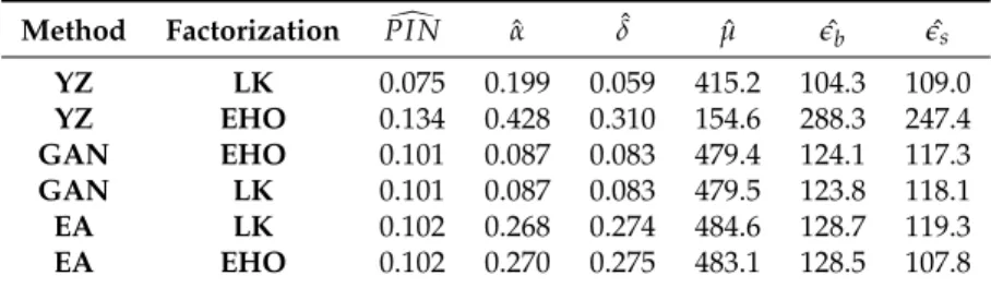
The results are presented in Table1which indicates that YZ() method with LK() factorization provides the PIN estimates with lowest MAE. Although the clustering algorithms, especially GAN() method, provide powerful estimates of ˆα, ˆδ, ˆeb, ˆes, they fail to estimate the arrival rate of informed
investors ˆµ,accurately. This is in line withErsan and Alici(2016). On the contrary, YZ() method with EHO()factorization provides the best estimates for ˆµ, but fails to provide good estimates for other parameters. Method Factorization PI Nd ˆα ˆδ µˆ eˆb eˆs YZ LK 0.075 0.199 0.059 415.2 104.3 109.0 YZ EHO 0.134 0.428 0.310 154.6 288.3 247.4 GAN EHO 0.101 0.087 0.083 479.4 124.1 117.3 GAN LK 0.101 0.087 0.083 479.5 123.8 118.1 EA LK 0.102 0.268 0.274 484.6 128.7 119.3 EA EHO 0.102 0.270 0.275 483.1 128.5 107.8
Table 1:This table represents the mean absolute errors (MAE) of the parameter estimates obtained by a given method for a given factorization. Each row represents a different method with a different factorization. First two column represent the specification of method and factorization respectively. The last six columns represents the power of estimates of PIN along with the parameter space Θ≡ {α, δ, µ, eb, es}. MAE measures for the estimates calculated as∑i=1N |Θbi−Θ
TR i |
N where bΘ represent
the estimates andΘTRrepresents the true value.
A more general way of examining the accuracy of PIN estimates is proposed in several studies (e.g,Lin and Ke(2011),Gan et al.(2015),Ersan and Alici(2016)). In this setting, we fix the trade intensity, I=2500. The total trade intensity represents the overall presence of informed and uninformed traders, that is, I=(µ, eb, es). We then generate three probability terms p1, p2, p3with N=5000 random
observations that are distributed uniformly between 0 and 1. p1represents the fraction of informed
investors in total trade intensity, that is, µ=p1∗I. The rest of the trade intensity is distributed equally
to buy and sell orders of uninformed investors, that is, eb=es = (1−p1) ∗I/2. p2represents the
true parameter for the probability of news arrival, α, and p3is the true parameter for the content of
the news, δ. We generate observations for ˜α and ˜δ, as described earlier. For each pair of ˜α and ˜δ, we generate buy and sell values(Bt, St)for hypothetical T=60 days, again, in the manner presented above;
form the likelihood and obtain the parameter estimates.
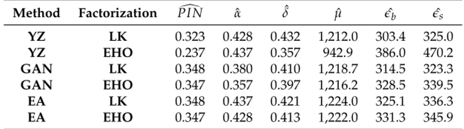
The results are presented in Table2. Similar to first simulation, GAN() captures the true nature of ˆα and ˆδ better than any other method with both factorizations. YZ() method with EHO() factorization performs best when estimating the arrival of informed traders, ˆµ. The importance of estimating
ˆ
µbecomes quite evident in Table2. Although other methods outperform YZ() method with EHO() factorization in estimating α, eband es, it provides the best estimate for PIN due to it’s performance on
estimating ˆµ.
Summary
This paper provides a short survey on five most widely used estimation techniques for the probability of informed trading (PIN) measure. In this paper, we introduce the R package InfoTrad, covering estimation procedures for PIN using EHO, LK factorizations along with YZ, GAN and EA algorithms (EHO(),LK(), YZ(), GAN() EA()). The functions EHO() and LK() read a (Tx2) matrix where the rows of the first column contains total number of buy orders on a given trading day t, Bt, and the rows
Method Factorization PI Nd ˆα ˆδ µˆ eˆb eˆs YZ LK 0.323 0.428 0.432 1,212.0 303.4 325.0 YZ EHO 0.237 0.437 0.357 942.9 386.0 470.2 GAN LK 0.348 0.380 0.410 1,218.7 314.5 323.3 GAN EHO 0.347 0.357 0.397 1,216.2 328.5 339.5 EA LK 0.348 0.437 0.421 1,224.0 325.1 336.3 EA EHO 0.347 0.428 0.413 1,222.0 331.3 345.9
Table 2:This table represents the mean absolute errors (MAE) of the parameter estimates obtained by a given method for a given factorization. Each row represents a different method with a different factorization. First two column represent the specification of method and factorization respectively. The last six columns represents the power of estimates of PIN along with the parameter space Θ≡ {α, δ, µ, eb, es}. MAE measures for the estimates calculated as∑i=1N |Θbi−Θ
TR i |
N where bΘ represent
the estimates andΘTRrepresents the true value.
of the second column contains the total number of sell orders on a given trading day t, St, where
t ∈ {1, 2, . . . , T}. In addition, they also require an initial parameter vector in the form of, Θ0 =
{α, δ, µ, eb, es}. Both functions produce the respective log-likelihood functions.
The functions YZ(), GAN() and EA() read(Bt, St)as an input along with a likelihood specification
that is set to ‘LK’ by default. These functions do not require initial parameter matrix to obtain the parameter estimates when calculating PIN. All three functions use neldermead() method of nloptr as built-in optimization procedure for MLE. YZ() GAN() and EA() produce an object that gives the parameter estimates ˆΘ along with likelihood value andPI N.d
Acknowledgments
This research is supported by the Scientific and Technological Research Council of Turkey (TUBITAK), Grant Number: 116K335.
Bibliography
N. Aktas, E. De Bodt, F. Declerck, and H. Van Oppens. The PIN anomaly around m&a announcements. Journal of Financial Markets, 10(2):169–191, 2007. URLhttps://doi.org/10.1016/j.finmar.2006. 09.003. [p31]
J. Duarte and L. Young. Why is PIN priced? Journal of Financial Economics, 91(2):119–138, 2009. URL https://doi.org/10.1016/j.jfineco.2007.10.008. [p31]
D. Easley, N. M. Kiefer, M. O’Hara, and J. B. Paperman. Liquidity, information, and infrequently traded stocks. The Journal of Finance, 51(4):1405–1436, 1996. URL https://doi.org/10.1111/j.1540-6261.1996.tb04074.x. [p31,32,34]
D. Easley, M. O’Hara, and J. Paperman. Financial analysts and information-based trade. Journal of Financial Markets, 1(2):175–201, 1998. URLhttps://doi.org/10.1016/s1386-4181(98)00002-0. [p31]
D. Easley, M. O’Hara, and G. Saar. How stock splits affect trading: A microstructure approach. Journal of Financial and Quantitative Analysis, 36(01):25–51, 2001. URLhttps://doi.org/10.2307/2676196. [p31]
D. Easley, S. Hvidkjaer, and M. O’Hara. Is information risk a determinant of asset returns? The Journal of Finance, 57(5):2185–2221, 2002. URLhttps://doi.org/10.1111/1540-6261.00493. [p31,32] D. Easley, S. Hvidkjaer, and M. O’Hara. Factoring information into returns. Journal of Financial and
Quantitative Analysis, 2010. URLhttps://doi.org/10.1017/s0022109010000074. [p31,33] A. Ellul and M. Pagano. IPO underpricing and after-market liquidity. Review of Financial Studies, 19(2):
381–421, 2006. URLhttps://doi.org/10.1093/rfs/hhj018. [p31]
O. Ersan and A. Alici. An unbiased computation methodology for estimating the probability of informed trading (PIN). Journal of International Financial Markets, Institutions and Money, 43:74–94, 2016. URLhttps://doi.org/10.1016/j.intfin.2016.04.001. [p31,32,33,34,40]
T. Foucault, M. Pagano, and A. Röell. Market Liquidity: Theory, Evidence, and Policy. Oxford University Press, 2013. URLhttps://doi.org/10.1093/acprof:oso/9780199936243.001.0001. [p32] Q. Gan, W. C. Wei, and D. Johnstone. A faster estimation method for the probability of informed
trading using hierarchical agglomerative clustering. Quantitative Finance, 15(11):1805–1821, 2015. URLhttps://doi.org/10.1080/14697688.2015.1023336. [p31,32,34,39,40]
C. Lee and M. J. Ready. Inferring trade direction from intraday data. The Journal of Finance, 46(2): 733–746, 1991. URLhttps://doi.org/10.1111/j.1540-6261.1991.tb02683.x. [p31]
H.-W. W. Lin and W.-C. Ke. A computing bias in estimating the probability of informed trading. Journal of Financial Markets, 14(4):625–640, 2011. URLhttps://doi.org/10.1016/j.finmar.2011.03.001. [p31,33,40]
A. J. Menkveld. Splitting orders in overlapping markets: A study of cross-listed stocks. Journal of Financial Intermediation, 17(2):145–174, 2008. URLhttps://doi.org/10.1016/j.jfi.2007.05.004. [p32]
D. Müllner. Fastcluster: Fast hierarchical, agglomerative clustering routines for r and python. Journal of Statistical Software, 53(9):1–18, 2013. URLhttps://doi.org/10.18637/jss.v053.i09. [p34,35] E. R. Odders-White and M. J. Ready. Credit ratings and stock liquidity. Review of Financial Studies, 19
(1):119–157, 2006. URLhttps://doi.org/10.1093/rfs/hhj004. [p31]
R Core Team. R: A Language and Environment for Statistical Computing. Vienna, Austria, 2016. [p32] Y. Yan and S. Zhang. An improved estimation method and empirical properties of the probability
of informed trading. Journal of Banking & Finance, 36(2):454–467, 2012. URLhttps://doi.org/10. 1016/j.jbankfin.2011.08.003. [p31,32,33]
P. Zagaglia. FinAsym, 2012. URLhttps://CRAN.R-project.org/package=FinAsym. R package ver-sion 1.0. [p31,32,33]
P. Zagaglia. PIN: Measuring Asymmetric Information in Financial Markets with R. The R Journal, 5(1):80–86, 2013. URLhttps://journal.r-project.org/archive/2013/RJ-2013-008/index.html. [p31,32]
Duygu Çelik Bilkent University
Bilkent University Department of Management 06800 Bilkent Ankara Turkey
Murat Tiniç Bilkent University
Bilkent University Department of Management 06800 Bilkent Ankara Turkey