https://doi.org/10.1080/1331677X.2018.1427610
An analysis of biomass consumption and economic growth in
transition countries
Melike Bildiricia and Fulya Özaksoyb
aEconomics, Yildiz technical University, istanbul, turkey; bDepartment of Economics and Finance, Dogus University, istanbul, turkey
ABSTRACT
In this paper, the relationship between biomass energy consumption and economic growth was analysed for some European Transition Countries. Two econometrical methods, which are time series (Autoregressive Distributed Lag (A.R.D.L.) bounds testing approach and Granger Causality) and Panel data methods (Pedroni test, Panel Johansen test and Panel Causality test) were used to determine the cointegration relationship between the variables. A.R.D.L. and Granger Causality methods were practiced for Albania, Bulgaria and Romania for the 1981–2014 period. Panel Cointegration and Causality methods were applied for Bosnia and Herzegovina, Czech Republic, Hungary, Macedonia and Slovak Republic for the 1991–2014 period; and Croatia, Estonia, Latvia and Slovenia for the 1995–2014 period. According to the results, while short-run and long-run causality results demonstrate that the conservation hypothesis is valid for Albania and the countries in group 1, evidence of the growth hypothesis is supported for Bulgaria, Romania and the countries in group 2. In strong causality results, evidence of bidirectional causality for all countries is found.
1. Introduction
Biomass energy consumption is a significant part of energy consumption and is as old as humanity. However, traditional biomass energy consumption is not commonly used around the world because it has not met energy needs of the economy in recent years. As the economy has developed, fossil energy has gained popularity and traditional biomass energy consumption has diminished. Because of rapid urbanisation, traditional usage of biomass energy has lost its popularity. Further, because of problems such as environmental pollution, limited fossil reserves, increased oil prices and the Chernobyl disaster caused by fossil energy, worldwide interest has steered away from fossil energy sources such as coal, oil and natural gas to renewable energy resources like biomass, geothermal, solar power,
KEYWORDS
Biomass; transition countries; a.R.D.L.; Panel Granger causality; Pedroni test; Panel johansen test JEL CLASSIFICATIONS c32; c33; Q43; Q48; P28 ARTICLE HISTORY Received 7 july 2015 accepted 18 january 2017
© 2018 the author(s). Published by informa Uk Limited, trading as taylor & Francis Group.
this is an open access article distributed under the terms of the creative commons attribution License (http://creativecommons.org/
licenses/by/4.0/), which permits unrestricted use, distribution, and reproduction in any medium, provided the original work is properly cited.
CONTACT melike Bildirici [email protected]
wind and hydropower because renewable and sustainable energy is mainly regarded as a key factor for the future of the world (Bildirici & Ersin, 2015; Bildirici & Ozaksoy, 2013).
Biomass energy has a significant role, not only in the meaning of wealth, but also as a remarkable factor in economic growth. Besides other positive effects of biomass energy, it diminishes foreign dependency on oil and, especially in developing countries, modern biomass energy can benefit rural employment. Furthermore, biomass energy is highly appre-ciated because it contributes to poverty reduction and meets energy needs more economi-cally. Biomass offers sustainable development as an important alternative of non-renewable energy resources. It provides opportunities for wide-ranging forms of energy. Additionally, it assists in developing biodiversity, soil fertility and water embowering (Balat, 2005; Bildirici & Ozaksoy, 2014). As other types of renewable energy, biomass energy consumption also has important effects on the economy.
The aim of this paper is to investigate the relationship between biomass energy consump-tion and economic growth in the transiconsump-tion countries.
The contribution of this study is in being the first paper focused on biomass energy by analysing the transition countries and discussing the importance of the relationship between economic growth and biomass energy consumption by four econometrical methods, which are the Autoregressive Distributed Lag (A.R.D.L.), Granger Causality, Panel Cointegration tests (Pedroni and Panel Johansen tests) and Panel Causality test. It is important to identify the direction of causality and long-term coefficients for each of the analysed countries, because this point of view makes significant contributions to the economy, especially in the context of energy politics proposals. However, because of data scarcity of the analysed countries, we preferred to test by Panel Cointegration and Panel Causality to make economic policy suggestions. The data for some selected transition countries does not cover the period 1981–2014. The A.R.D.L. method preference is not feasible for very small samples; in this situation the Panel model was used. The data covering the 1981–2014 period was tested by the A.R.D.L. method for Albania, Bulgaria and Romania, but the other countries’ data covers the time after 1990 for which countries panel analyses were preferred. The panel cointegration method was applied for Bosnia and Herzegovina, Czech Republic, Hungary, Macedonia and Slovak Republic for the 1991–2014 period; and for Croatia, Estonia, Latvia and Slovenia for the 1995–2014 period.
The next section is the literature review. Econometric theory and methodology are iden-tified in the third section and a further section consists of the empirical results, while the last section includes the conclusion and policy implications.
2. Literature review
Even if there are many papers that have analysed the relationship between energy consump-tion and economic growth, only a few of them explain the relaconsump-tionship between renewable energy consumption and economic growth and some of them deal with the relationship between biomass energy consumption and economic growth. The studies lay emphasis on four different hypotheses which are constructed as the ‘growth hypothesis’, ‘conservation hypothesis’, ‘feedback hypothesis’ and ‘neutrality hypothesis’. First, the growth hypothesis accepts uni-directional causality from biomass energy consumption to economic growth. Biomass energy consumption has a significant impact on economic growth and an increase in biomass energy consumption causes a rise in economic growth. Second, the conservation
hypothesis postulates that biomass energy consumption is driven by economic growth. There is uni-directional causality from economic growth to biomass energy consumption. Third, the feedback hypothesis accepts an interdependent relationship between biomass energy consumption and economic growth. In such a case, energy conservation policies may decrease economic growth performance and the changes in economic growth may decrease energy consumption. Fourth, the neutrality hypothesis asserts that biomass energy consumption serves a relatively minor role in economic growth.
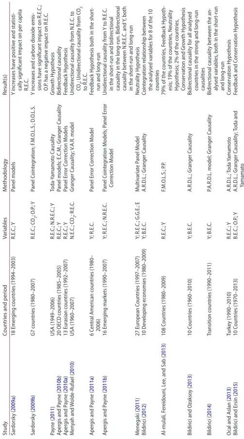
Table 1 indicates the relationship between renewable energy consumption and economic growth in these studies.
In the studies which researched the relationship between biomass energy consumption and economic growth, the causality relationship between biomass energy consumption and real G.D.P. (gross domestic product) was tested by Bildirici (2012, 2013, 2014, 2016), Bildirici and Ozaksoy (2013, 2014), Bildirici and Ersin (2015), Bilgili and Ozturk (2015) and Öztürk and Bilgili (2015).
Bildirici (2012) tested the long-run and short-run causality relationship between biomass energy consumption and economic growth and she found the cointegrated relationship between biomass energy consumption and the economic growth for nine of the 10 countries. Bildirici (2013) investigated the relationship between biomass energy consumption and real G.D.P. for the Central American countries, Argentina, Bolivia, Brazil, Chile, Colombia, Guatemala and Jamaica. Bidirectional causality between the analysed variables was found for all of the analysed countries in the long-run in this study. Bildirici and Ozaksoy (2013) tested the relationship between biomass energy consumption and economic growth in 10 selected European countries. According to strong and long-run causality, a bidirectional relationship between the variables was determined for all of the analysed countries.
Bildirici (2014) analysed the co-integration and causality relationship between biomass energy consumption and economic growth in the transition countries for the period from 1990–2011. Fully modified ordinary least square results of the study show that biomass energy consumption has a positive effect on the economic growth. Bildirici and Ozaksoy (2014) examined the relationship between biomass energy consumption and economic growth for the European transition countries in the period 1980–2011. The causality results suggest evidence of the conservation hypothesis from economic growth to biomass energy consumption for Slovenia and Slovakia; and for the growth hypothesis from biomass energy consumption to economic growth for Bulgaria and Romania.
Bildirici and Ersin (2015) discussed the relationship among biomass energy consump-tion, oil prices and economic growth in Austria, Canada, Germany, Great Britain, Finland, France, Italy, Mexico, Portugal and the USA for the 1970–2013 period. For Austria, Germany, Finland and Portugal, the Granger Causality test determined that the conservation hypoth-esis is supported. In the USA, the feedback hypothhypoth-esis highlights the interdependent rela-tionship between biomass energy consumption and economic growth. The Tado Yamamoto test determined the conservation hypothesis for Austria, Germany, Finland and Portugal. In the USA, the feedback hypothesis highlights the interdependent relationship between biomass energy consumption and economic growth.
Öztürk and Bilgili (2015) investigated the long-run dynamics of economic growth and biomass consumption by applying dynamic panel analyses for 51 Sub-Sahara African coun-tries for the 1980–2009 period. The results show that economic growth is affected by biomass
Table 1. Renew able ener gy c onsumption and ec onomic g ro wth. Study Coun tr
ies and per
iod Var iables M ethodology Result(s) sar dorsk y ( 2009a ) 18 Emer ging c oun tries (1994–2003) R.E. c.; Y Panel models Y incr eases ha ve positiv e and sta tisti -cally sig nifican t impac t on per capita R.E. c. sar dorsk y ( 2009b ) G7 c oun tries (1980–2007) R.E. c.; co2 ; o .P.; Y Panel coin teg ra tion; F .m .o .L. s.; D .o .L. s. Y incr
eases and carbon dio
xide emis -sions ha ve sig nifican t impac t on R.E. c.; o .P. has a nega tiv e impac t on R.E. c. Pa yne ( 2011 ) U sa (1949–2006) R.E. c.; n .R.E. c.; Y toda-Yamamot o causalit y Gr owth h ypothesis aper gis and P ayne ( 2010b ) 20 o Ec D c oun tries (1985–2005) R.E. c.; Y Panel models; E. c. m .; Gr anger causalit y Bidir ec tional causalit y aper gis and P ayne ( 2010a ) 13 E ur asian c oun tries (1992–2007) R.E. c.; Y Panel Err or corr ec tion m odels Feedback h ypothesis m en yah and W olde -Rufael ( 2010 ) U sa (1960–2007) n .E. c.; co 2 ; R.E. c. Gr anger causalit y; v. a.R. model Unidir ec tional causalit y fr om n .E. c. t o co 2 ; Unidir ec tional causalit y fr om co2 to R.E. c. aper gis and P ayne ( 2011a ) 6 cen tr al american c oun tries (1980– 2006) Y; R.E. c. Panel Err or corr ec tion m odel Feedback h
ypothesis both in the shor
t-run and long-t-run
aper gis and P ayne ( 2011b ) 16 Emer ging mark ets (1990–2007) Y; R.E. c.; n .R.E. c. Panel coin teg ra tion m odels; P anel Err or corr ec tion m odel Unidir ec tional causalit y fr om Y t o R.E. c. in the shor
t-run and bidir
ec
tional
causalit
y in the long-run. Bidir
ec tional causalit y bet w een n .R.E. c. and Y, both in the shor
t-run and long-run
m enegak i ( 2011 ) 27 E ur opean coun tries (1997–2007) Y; R.E. c.; G.G.E.; E m ultiv aria te P anel m odel n eutr alit y h ypothesis Bildirici ( 2012 ) 10 D ev eloping ec onomies (1980–2009) Y; B .E. c. a.R.D .L.; Gr anger causalit y coin teg ra tion r ela tionship bet w een the analy sed v ariables f or 8 of the 10 coun tries al-mulali, F er eidouni, L ee , and sab ( 2013 ) 108 coun tries (1980–2009) R.E. c.; Y F.m .o .L. s.; P .P. 79% of the c oun tries , F eedback h ypoth -esis; 19% of the c oun tries , n eutr alit y h ypothesis; 2% of the c oun tries , conser va tion and Gr owth h ypothesis Bildirici and o zakso y ( 2013 ) 10 coun tries (1960–2010) Y; B .E. c. a.R.D .L.; Gr anger causalit y Bidir ec tional causalit y f or all analy sed coun tries in the str
ong and long-run
causalities Bildirici ( 2014 ) tr ansition c oun tries (1990–2011) Y; B .E. c. P.a .R.D .L. model; Gr anger causalit y Bidir ec tional causalit y bet w een the an -aly sed v ariables
, both in the shor
t-run and long-run o cal and aslan ( 2013 ) turk ey (1990–2010) R.E. c.; Y a.R.D .L.; toda Y amamot o conser va tion h ypothesis
Bildirici and Ersin (
2015 ) 10 coun tries (1970–2013) B.E. c.; o .P.; Y a.R.D .L.; Gr anger causalit y; toda and Yamama to Feedback and conser va tion h ypothesis
R.E. c., Renew able Ener gy consumption; n .E. c., n uclear Ener gy consumption; co2 , co 2 Emissions; Y, Real G.D .P.; o .P., Real o il P ric e; E, Emplo ymen t; B .E. c., Biomass Ener gy consumption; n .R.E. c., n on-Renew able Ener gy consumption; c. s., capital st ock ; h .c ., h uman capital; c., capital U se; t. o ., tr ade o penness; G.G.E., Gr een h ouse G as Emissions; E. c. m ., Err or corr ec tion m odel; a.R.D .L., aut or eg ressiv e Distribution Lag; P .a .R.D .L., P anel aut or eg ressiv e Distribution Lag; D .o .L. s., D ynamic o .L. s.; F .m .o .L. s., F ully m odified o .L. s.; P .P., P hillips P err on. sour ce: authors . Ö ztürk and Bilg ili ( 2015 ) 51 sub -s ahar an african coun tries (1980–2009) Y; B .E. c. Panel analy sis Unidir ec tional r ela tion fr om B .E. c. t o Y Bilg ili and o zturk ( 2015 ) G7 coun tries (1980–2009) Y; c. s.; h .c .; B .E. c. Panel m odels Gr owth h ypothesis aslan ( 2016 ) the U sa (1961–2011) Y; B .E. c.; c. s.; h .c . a.R.D .L. Gr owth h ypothesis shahbaz, R asool , a hmed , and m ahalik ( 2016 ) B.R. i.c .s . Reg ion (1991–2015) Y; B .E. c.; c; t. o . Panel m odels Feedback h ypothesis bet w een B .E. c. and Y ali, La w , Y usop , and chin ( 2016 ) sub -s ahar an african coun tries (1980–2011) Y; B .E. c.; h .c .; c. s. D ynamic h et er ogeneous P anel m odels; D. o .L. s.; F .m .o .L. s B.E. c., h .c . and c. s. positiv ely influenc es Y Bildirici ( 2016 ) austr alia, canada, D enmark , F inland , Fr anc e, japan, the U k and the U s Y; B .E. c. a.R.D .L.; Gr anger causalit y in shor t-run causalit y, f or canada, Fr anc e, the U k and the U s, c onser -va tion h ypothesis and f or austr alia, Belg ium, F inland and japan, the gr owth h ypothesis . i n str ong causalit y, bi-dir ec tional causalit y f or the U s, the U k and F ranc e Table 1. (C ontin ued ).
consumption, openness and population, both significantly and positively in these African countries.
Bilgili and Ozturk (2015) determined the long-run dynamics of biomass energy con-sumption and G.D.P. growth through homogeneous and heterogeneous variance structures of the G7 countries for the 1980–2009 period by Panel unit root and Panel Cointegration analyses. The results confirmed the growth hypothesis in which biomass energy consump-tion has positive effects on the economic growth for the G7 countries.
Shahbaz, Rasool, Ahmed, and Mahalik (2016) studied the relationship between biomass energy consumption and economic growth for the B.R.I.C.S. (Brazil, Russia, India, China and South Africa) countries. The econometric results demonstrate that biomass energy consumption stimulates economic growth and the feedback hypothesis is supported for the relationship between biomass energy consumption and economic growth.
The results of Table 1 indicate that there is a bidirectional relationship between biomass energy and economic growth in 81.25% of the related studies. These findings confirm the importance of the relationship between biomass energy consumption and economic growth.
The papers in Table 1 used time series or panel data analysis methods. This paper is the first which uses two econometrical methods at the same time: the time series (A.R.D.L., Granger Causality) and Panel data analyses (Pedroni, Panel Granger and Panel Johansen tests) to test the relationship between economic growth and biomass energy consumption in the transition countries.
3. Data and econometric methodology
3.1. Data
In this paper, the relationship between biomass energy consumption and per capita G.D.P. was analysed by A.R.D.L. and Panel Cointegration approaches for some of the transition countries. The data of the 1981–2014 period could not be obtained for all of the analysed countries. For the countries whose data covers the period 1981–2014, the A.R.D.L. method was preferred and it was used for 35 years. However, the Panel method was used for the data of the 24 yearly and 20 yearly periods and two separate groups were comprised. Accordingly, Panel tests were applied to Bosnia and Herzegovina, Croatia, Czech Republic, Estonia, Hungary, Latvia, Macedonia, Slovak Republic and Slovenia. The countries of Group 1 are Bosnia and Herzegovina, Czech Republic, Hungary, Macedonia and Slovak Republic. Panel Cointegration analyses were applied to these countries during the 1991–2014 period. Group 2 consists of Croatia, Estonia, Latvia and Slovenia and the Panel Cointegration method was applied for the 1995–2014 period.
The data was taken from the Worldbank World Development Indicators. BC and Y show biomass energy consumption and per capita G.D.P., respectively. We used logarithmic transformation of the variables: bc is log (BCt) and y is log (Yt).
3.2. Methodology
Time series data and panel data methodologies, which were applied in this study, are as below.
3.2.1. A.R.D.L. methodology
The A.R.D.L. cointegration approach, which has numerous advantages over other coin-tegration methods, is commonly used in energy economics literature. First, the A.R.D.L. procedure can be applied if the regressors are I(1) and/or I(0), while the Johansen (1988), Johansen and Juselius (1990) cointegration techniques require that all variables in the system be in equal order of integration (Bildirici & Kayıkcı, 2012). The A.R.D.L. method does not need unit root pre-testing. Second, while the Johansen cointegration techniques require large samples for validity, the A.R.D.L. procedure is statistically more effective in determining the cointegration relationship in small samples. Third, the A.R.D.L. procedure allows the vari-ables to have different optimal lags. Finally, the A.R.D.L. procedure employs only a single- reduced form of equation, while the other cointegration procedures estimate the long-run relationship within a context of system equations (Bildirici & Ersin, 2015; Narayan, 2005).
The A.R.D.L. approach to cointegration involves three steps for estimating the long-run relationship. The first step is to investigate the existence of a long-run relationship among all variables in the equation under estimation (Pesaran & Shin, 1999). In the A.R.D.L.-U.E.C.M. (Unrestricted Error Correction Model) method, the standard log-linear functional specification for the ‘bc’ variable is presented as:
where 𝛥and 𝜀1t are the first difference operator and the white noise term, respectively. The null hypothesis of no cointegration among the variables in equation (1) is H0: 𝜙=𝜑= 0 against the alternative hypothesis H1: 𝜙 ≠ 𝜑 ≠ 0. If the calculated F-statistics are below the upper CV, we cannot reject the null hypothesis of no cointegration.
In the second step, if cointegration is established, the conditional A.R.D.L. long-run model for ‘bc’ can be estimated as:
In the third stage, the short-run dynamic parameters are obtained by estimating an error correction model associated with the long-run estimates:
where the residuals are independently and normally distributed with zero mean and con-stant variance and ECMt−1 is the error correction term. ζ is a parameter that indicates the speed of adjustment to the equilibrium level after a shock. It shows how quickly the vari-ables converge to equilibrium and it must have a statistically significant coefficient with a negative sign. (1) Δbct = 𝛼 + m ∑ i = 1 𝛽Δbct - i+ n ∑ j = 0 𝛾Δyt - j+ 𝜙bct - 1+ 𝜑yt - 1+𝜀1t (2) bct= 𝜆0+ m ∑ i = 1 𝛼ibct - i+ n ∑ i = 0 𝜗iyt - i+ ut (3) Δbct= 𝜆0+ m ∑ i = 1 𝛼iΔbct - i+ n ∑ i = 0 𝜗iΔyt - i+ 𝜁ECMt−1+ et
3.2.2. Granger causality
The Vector Error Correction model should be a starting point for causality analysis (Lee & Chang, 2008; and Bildirici (2012, 2013)). The Vector Error Correction model was con-structed as follows:
where residuals et are independently and normally distributed with zero mean and constant variance and ECMt−1 is the error correction term resulting from the long-run equilibrium relationship. (1) Short-run or weak Granger causalities are detected by testing H0: 𝜙i =0 and H0: 𝜃i =0 for all i and j in equations (4) and (5). Long-run causalities are examined by testing H0: 𝜁1 =0 and H0: 𝜁2 =0. (3) Strong Granger causalities are detected by testing H0: 𝜙i=𝜁1=0 and H0: 𝜙i=𝜁2=0 for all i and j in equations (4) and (5).
3.3. Panel cointegration and Granger causality 3.3.1. Pedroni test
The Pedroni test is the most popular one in panel cointegration. Pedroni (1999, 2004) derived seven panel cointegration statistics. In its most general form, we will consider the following type of regression (Pedroni, 2004):
for a time series panel of observations yit and Xit for members i = 1, ..., N over time periods
t = 1, ..., T, where Xit is an m-dimensional column vector for each member i and βi is an m-dimensional row vector for each member i. The variables yit and Xit are assumed to be integrated of order one, denoted by I(1), for each member i of the panel and, under the null hypothesis of no cointegration, the residual eit will also be I(1). The parameters αi and δi allow for the possibility of member-specific fixed effects and deterministic trends, respectively. The slope coefficients βi are also permitted to vary by individual country, so that, in general, the cointegrating vectors may be heterogeneous across members of the panel (Pedroni, 2004).
For the null hypothesis H0: ‘all of the individuals of the panel are not cointegrated’. For the alternative hypothesis is simply H1: ‘all of the individuals are cointegrated’. For the alter-native hypothesis should be H1: ‘a significant portion of the individuals are cointegrated’ (Pedroni, 2004).
To test the null hypothesis of no cointegration, the following unit root test is conducted on the residuals as follows: 𝜀it= 𝜌i𝜀it−1+uit. The first category of four statistics is defined as within-dimension-based statistics and includes a variance ratio statistic, a non-parametric Phillips and Perron type ρ statistic, a non-parametric Phillips and Perron type t-statistic and a DF type t-statistic. The second category of three panel cointegration statistics is defined as between-dimension-based statistics and is based on a group mean approach (Bildirici, 2004a, 2004b; Bildirici & Bohur, 2014). Pedroni’s (2004) heterogeneous panel and
(4) Δyt= 𝛼0+ m ∑ i = 1 𝛽iΔyt - i+ n ∑ j = 1 𝜙iΔbct - j+ 𝜍1ECMt - 1+ e1t (5) Δbct= 𝛼0+ p ∑ i = 1 𝜗iΔbct - i+ q ∑ j = 1 𝜃iΔyt - j+ 𝜍2ECMt - 1+ e2t (6) yit= 𝛼i+ 𝛿it + 𝛽iXit+eit
heterogeneous group mean panel cointegration statistics are then calculated. Both kinds of tests focus on the null hypothesis of no cointegration. The finite sample distribution for the seven statistics has been tabulated by Pedroni via Monte Carlo simulations (Bildirici & Kayıkci, 2012).
Asymptotic distributions of residual-based tests for the null hypothesis of no cointegra-tion in heterogeneous panels are given in Pedroni (2004).
The calculated test statistics must be smaller than the tabulated critical value to reject the null hypothesis of the absence of cointegration.
3.3.2. Panel Johansen test
Following the Bildirici, Ersin, and Kokdener (2011) procedure, consider a V.A.R. (Vector Auto Regressive Models) model with Gaussian errors
As shown by Johansen (1991), if the process is written in error correction form, the equa-tion becomes
where ɛt(t = 1, ..., T) are independent p-dimensional Gaussian variables with mean zero and variance matrix Λ. Dt are defined as deterministic components which are seasonal dummies orthogonal to the constant term, 𝛱= −I +∑ki=1𝛱i and 𝛤i= −∑kj=i+1𝛱i, where Γi, θ, μ
and Λ are assumed to vary without restrictions. In order to show that Xt ∼ I(1) integrated to the order 1, the assumptions are:
(1) det (A(z)) = det (I − Π1z − Π1z2 − .... − Π
kzk) are either outside the unit circle or equal to 1, which guarantees that the process is not explosive;
(2) the Π matrix has reduced rank, r < p, and can be presented as the product Π = αβ′; therefore, there are at least p–r unit roots which leads to cointegration if r ≥ 1 and (3) the α′Γβ′ matrix has full rank, where α′ and β′ are orthogonal complements to α
and β, so that the process is restricted to the order of integration of 1.
If the model in equation (8) is denoted as H1, then, by applying restrictions on Π, the hypoth-esis to test (at most) r cointegration vectors, produces H2:Π = αβ′, where β and α are p × r. matrices which denote the cointegrating vectors and adjustment coefficients, respectively (Bildirici et al., 2011; Johansen, 1991).
Extending the V.A.R. model in equation (8), for a panel dataset with N cross sections and T time periods, a panel V.A.R. is written as
with i = 1,2,…,N groups and t = 1,2,…,T time periods and j = 1,2,…,p variables, the errors are independently identically distributed ɛit ∼ NP(0, Ωi). Error representation of the V.A.R. model following Engle and Granger (1987) and Johansen (1991) is
(7) Xt = Π 1 Xt−1+ Π2 Xt−2+... + Πk Xt−k+Dt+ 𝜀t, t = 1, ...., T (8) ΔXt =∑k−1 i=1 ΓiΔXt−i+ ΠXt−k+ 𝜃Dt+ 𝜇 + 𝜀t, t = 1, ..., T (9) Xit=∑ki k=1ΠikXi,t−k+ 𝜀it (10) Xit= ΠiXi,t−1+∑ki−1 k=1ΓikΔXi,t−k+ 𝜀it
where Πi is of order p × r. If Πi has reduced rank, then extending the assumption i for panels, we obtain, 𝛱i = 𝛼i𝛽i� where αi are the adjustment parameters and β′ are the long-run
param-eters, respectively. αi and β′ are of order p × r
i and full column rank. The Cointegrating rank hypothesis is stated as H(r):rank(Π) ≤ r and tested against the alternative H(r):rank(Π) = r, where the likelihood ratio test, called the trace statistic is
where, 𝜆̂
i trace statistic is the ith eigenvalue to a certain eigenvalue problem (Bildirici et al.,
2011; Larsson & Lyhagen, 2007; Larrson, Lyhagen, & Lothgren, 2001). 3.3.3. F.M.O.L.S.
Pedroni proposed the Fully Modified Ordinary Least Squares (F.M.O.L.S.) estimator sug-gested by Phillips and Hansen (1990) for the heterogeneous panel. F.M.O.L.S. results pro-duce consistent standard errors and t-statistics in the presence of endogenous regressors (Purna & Pravakar, 2007). We start with the Ordinary Least Squares (O.L.S.) regression in Pedroni (2004)
and these are cointegrated with slopes βi. Let 𝜀it = ̂uit, 𝛥Xit be a stationary vector including the estimated residuals and differences. Also, let
F.M.O.L.S. estimators are given as:
where
The between-dimension estimator is 𝜙̇GFM = N−1 N ∑ i=1
𝜙𝜅M,t, where 𝜙𝜅M,t is the F.M.O.L.S. estimator. The associated t-statistic for the between-dimension estimator is given as
(11) −2InQT{H(r) | H(p)}= −T∑p i=r+1In(1 + ̂𝜆i) (12) yit = 𝛼i+ 𝛽iXit+ 𝜇it (13) Ωit= lim T→∞E [ T−1 ( T ∑ t=1 𝜀iT )( T ∑ t=1 𝜀iT )�] (14) 𝜙=N−1 N ∑ i=1 ( T ∑ i=1 (xit− ̄yi)2 )−1 x ( T ∑ i=1 (xit− ̄xi)2s∗it−T𝜆i ) (15) yit∗ = (sit− ̄si) − ̂ 𝛺21t ̂ 𝛺22t𝛥xit∗ ⌢ 𝜆t = ̂𝛤21t+ ̂𝛺̇21t− ̂ 𝛺21t ̂ 𝛺22t( ̂𝛤22t+ ̂𝛺̇22t) (16) ṫGFM = N−1∕2 N ∑ t=1 t𝜙̇𝜅M,t, where t ̂𝜙̇𝜅M,t= ( ̂𝜙̇𝜅M,i− 𝜙0) ( ̂ Ω−111t T ∑ t=1 (xit− ̄xi)2 )1∕2
3.3.4. Panel Granger causality results
The Vector Error Correction (V.E.C.) model used to analyse the relationships between the variables was constructed. First a panel vector error correction model is estimated to perform Granger-causality tests (Bildirici & Bohur, 2014). The Engle and Granger (1987) two-step procedure is used afterwards, defining the lagged residuals as the error correction term and the following dynamic error correction models are estimated:
where Δ is the first-difference operator; m is the lag length set at two based on likelihood ratio tests; and where the residuals ɛt are independently and normally distributed with zero mean and constant variance and ECMt−1 is the error correction term resulting from the long-run equilibrium relationship. Ϛ is a parameter indicating the speed of adjustment to the equilibrium level after a shock. Short-run or weak Granger causalities are obtained by testingH0: 𝜗1ik =0, in equation (17).
4. Econometric result
4.1. Time series results
The A.R.D.L. test was applied in four stages. First, the unit root test was applied. Second, bound test results were obtained. Third, long- and short-run results and E.C.M. results were obtained. Fourth, the Granger Causality test was practiced and the direction of causality was obtained.
4.1.1. Unit root test results
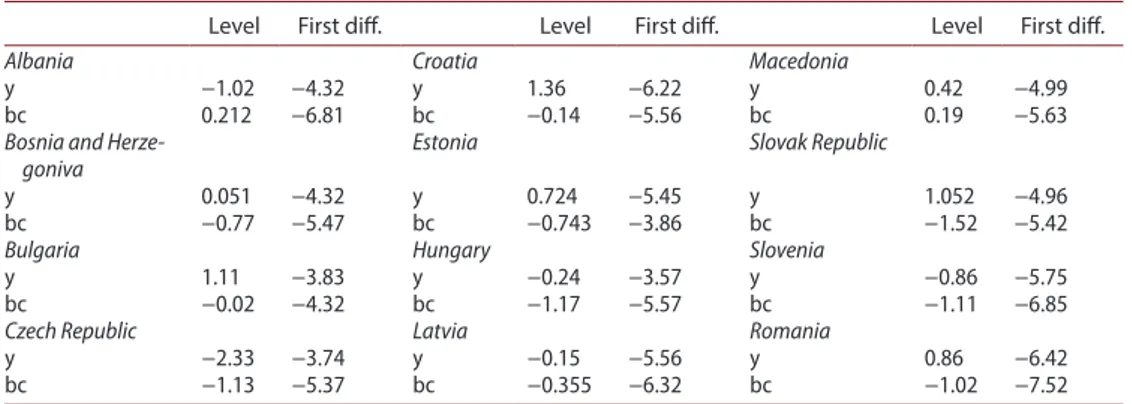
The unit root tests are used to determine if the variables are I(0) and/or I(1). The results of the A.D.F. (Augmented Dickey-Fuller) unit root tests are given in Table 2. The A.D.F. unit root tests conclude that the y and bc variables for the countries are stationary in the first differences.
4.1.2. A.R.D.L. results
According to the F-statistics, we have enough evidence to reject the null hypothesis of no cointegration at a 5% and 1% significance level for the relationship between biomass energy consumption and real per capita G.D.P. for Albania, Bulgaria and Romania.
This simply means that the computed F-statistics for these models are above the upper bound critical value. The results of the A.R.D.L. bounds tests for Albania, Bulgaria and Romania suggest evidence of the rejection of the null hypothesis. y is determined as a dependent variable for Bulgaria and Romania and bc is specified as a dependent variable for Albania in the Table 3.
(17) Δyit= 𝜆1j+ m ∑ k = 1 𝛼ikΔyit - k+ n ∑ k = 1
𝜗ikΔXit - k+ 𝜁0ECMit−1+𝜀1it
(18) Δbcit= 𝜆0+ m ∑ k = 1 𝛼2ikΔXt - k+ n ∑ k = 1
4.1.3. Long-run and E.C.M. results
Table 4 reveals the arguments for valid long-run relationships among the variables. It is possible to forecast the long- and short-run dynamic effects by using the A.R.D.L. approach. Table 4 shows the long-run elasticity for the A.R.D.L. model. The elasticities are interpreted as usual: for instance, a 1% increase in per capita income, when other things are equal, leads to a −0.2254% decrease in the consumption of biomass energy for Albania. According to this result, biomass energy consumption can be interpreted as ‘inferior good’. Bildirici and Ozaksoy (2014) indicated biomass energy consumption as ‘normal good’ for Hungary, Slovenia, Slovakia and Croatia, respectively. Additionally, a 1% increase in biomass energy consumption caused 0.6027% and 0.4687% growth in per capita income for Bulgaria and Romania, respectively.
The E.C.M.s in Table 5 indicate that there is a mechanism to correct the disequilibrium between economic growth and biomass energy consumption. The coefficient of the error correction term must change between −0.232 and −0.5073. The error correction term was Table 2. Unit root test result.
Level First diff. Level First diff. Level First diff.
Albania Croatia Macedonia
y −1.02 −4.32 y 1.36 −6.22 y 0.42 −4.99
bc 0.212 −6.81 bc −0.14 −5.56 bc 0.19 −5.63
Bosnia and Herze-goniva
Estonia Slovak Republic
y 0.051 −4.32 y 0.724 −5.45 y 1.052 −4.96 bc −0.77 −5.47 bc −0.743 −3.86 bc −1.52 −5.42
Bulgaria Hungary Slovenia
y 1.11 −3.83 y −0.24 −3.57 y −0.86 −5.75
bc −0.02 −4.32 bc −1.17 −5.57 bc −1.11 −6.85
Czech Republic Latvia Romania
y −2.33 −3.74 y −0.15 −5.56 y 0.86 −6.42
bc −1.13 −5.37 bc −0.355 −6.32 bc −1.02 −7.52 critical value for 1990–2014 period: −3.831,511 for 1% level; −3.029,970 for 5% level; −2.655,194 for 10% level and for
1980–2014 period: −3.639,407 for 1% level; −2.951,125 for 5% level; −2.614,300 for 10% level. source: authors.
Table 3. Bounds testing for cointegration.
* statistically significant.
the critical value for the F-test is 5.73 for 5% level and 4.78 for 10% level. the critical values of F-test are obtained from Pesaran, shin, and smith (2001).
source: authors.
Fy(y|bc) Fbc(bc|y)
albania 1.0523 18.7500*
Bulgaria 6.4850* 1.4365
Romania 5.8799* 0.0845
Table 4. Long-run coefficients for a.R.D.L.
t-values are given in parentheses.
the critical value for the F-test is 5.73 for 5% level and 4.78 for 10% level. the critical values of F-test are obtained from Pesaran et al. (2001). source: authors. c bc y R² (LM) albania 1.6115 (2.52) — −0.2254 (−2.9265) 0.810 Bulgaria 0.9056 (0.7637) 0.6027 (1.7647) — 0.702 Romania 0.5643 (1.8988) 0.4687 (1.9560) — 0.803
negative and statistically significant, showing a speed of adjustment of any disequilibrium towards a long-run equilibrium state, which is −0.232 for Albania, −0.3785 for Romania and −0.5073 for Bulgaria. Thus, for Bulgaria, the relationship between the variables will be approximately turned to equilibrium in 2 years.
4.1.4. Results for the Granger causality test
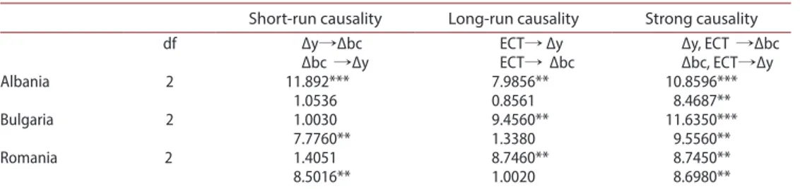
The A.R.D.L. methods do not indicate the direction of causality, but, since there is a long-run relationship between biomass energy consumption and economic growth, a causality relationship must exist in at least one direction. Therefore, we used the augmented Granger causality test by incorporating the error correction term. Table 6 summarises the causal relationship between biomass energy consumption and economic growth.
Table 6 exhibits the results determined by short-run, long-run and strong Granger cau-sality for selected countries. According to the short-run caucau-sality results, the evidence was accepted to reject the null hypothesis for a one-direction causal relationship between varia-bles for Albania, Bulgaria and Romania. For Albania, Bulgaria and Romania, the calculated Chi-square statistics are above the critical value with 2 degrees of freedom suggesting the rejection of the null hypothesis of no Granger causality between biomass consumption and economic growth at 5% significance level. It was found that there is evidence of uni-direc-tional causality from economic growth to biomass energy consumption for Albania.
Similarly, the results obtained for Bulgaria and Romania suggest evidence of uni-direc-tional causality from biomass energy consumption to economic growth at a 5% significance level. There is evidence of uni-directional causality from biomass energy consumption to economic growth for Bulgaria and Romania. Thus, the test results of this paper support the conservation hypothesis for Albania and the growth hypothesis for Bulgaria and Romania. The conservation hypothesis postulates that biomass energy consumption is driven by economic growth. According to the growth hypothesis, energy conservation policies may decrease economic growth performance. The long-run and strong Granger causality tests combined the variables and error correction terms to enhance the evidence in the Granger Table 5. E.c.m. and short-run results.
source: authors.
E.C.M. dbc dY R² (LM)
albania −0.232 (−1.954) — −0.035 (−4.721) 0.651 Bulgaria −0.507 (−1.878) 1.274 (1.878) — 0.694 Romania −0.379 (−1.901) −1.003 (−2.634) — 0.705
Table 6. Granger causality.
note: values in parentheses are t-values. significance levels: * p < 0.05; ** p < 0.01; and *** p < 0.001. For the co-joint test, we used the Wald-test (χ2).
in this table, the symbol → shows the direction of causality. source: authors.
Short-run causality Long-run causality Strong causality
df Δy→Δbc Ect→ Δy Δy, Ect →Δbc
Δbc →Δy Ect→ Δbc Δbc, Ect→Δy
albania 2 11.892*** 7.9856** 10.8596*** 1.0536 0.8561 8.4687** Bulgaria 2 1.0030 9.4560** 11.6350*** 7.7760** 1.3380 9.5560** Romania 2 1.4051 8.7460** 8.7450** 8.5016** 1.0020 8.6980**
causality test. The long-run and strong causality results determined the calculated Chi-square statistics are above the critical value with 2 degrees of freedom suggesting the rejec-tion of the null hypothesis of no Granger causality between biomass consumprejec-tion and economic growth at the 5% significance level. According to the long-run causality results, evidence was found to reject the null hypothesis for uni-directional causality between bio-mass energy consumption and economic growth in Albania, Bulgaria and Romania and there was evidence of the growth hypothesis for all countries. The results of strong Granger causality determined that, in Albania, Bulgaria and Romania, there was evidence to reject the null hypothesis for bidirectional causality between biomass energy consumption and economic growth. Strong causality results determined the feedback hypothesis. According to the feedback hypothesis, an energy policy focused on diminishing biomass energy con-sumption negatively affects the countries’ economic growth.
4.2. Panel data analysis
Panel analysis results were obtained in four stages. In the first stage, the Panel unit root test was applied. In the second stage, the results of the Pedroni Panel Cointegration test and Panel Johansen Cointegration test were used. In the third stage, F.M.O.L.S. test results were obtained and, in the last stage, Panel Granger Causality test results were acquired.
4.2.1. Panel unit root test results
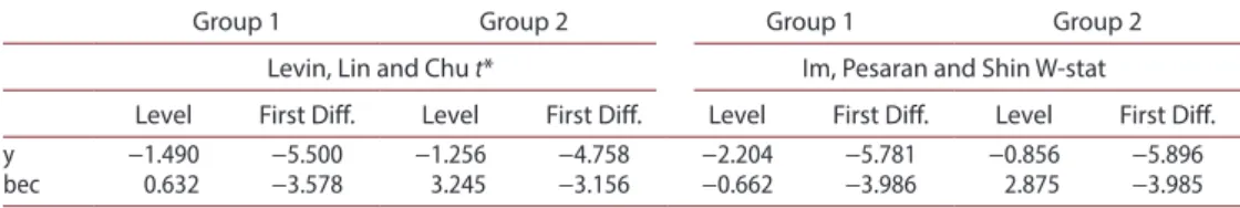
In this regard, Levin, Lin and Chu (L.L.C.) and Im, Pesaran and Shin (I.P.S.) unit root tests were examined in Table 7. The null hypothesis of unit root test cannot be rejected for the variables in levels. The unit root test is implemented in the first differences of the variables and the null hypothesis is rejected, implying that the levels are non-stationary and the first differences are stationary.
4.2.2. Pedroni cointegration results
Table 8a reports Pedroni test results for Groups 1 and 2. These statistics are based on aver-ages of the individual autoregressive coefficients associated with the unit root tests of the residuals for each of the countries in the panel. All seven panel cointegration tests reject the null hypothesis of no cointegration. Thus, the evidence suggests that, in both panel datasets, there is a long-run equilibrium relationship between biomass energy consumption and economic growth.
For Groups 1 and 2, Table 8b exhibits the Johansen test results. The Johansen cointegra-tion test results with 18.91 and 21.17 trace statistics and 17.66 C.V., which are significant Table 7. Panel unit root test.
source: authors.
Group 1 Group 2 Group 1 Group 2
Levin, Lin and Chu t* Im, Pesaran and Shin W-stat Level First Diff. Level First Diff. Level First Diff. Level First Diff. y −1.490 −5.500 −1.256 −4.758 −2.204 −5.781 −0.856 −5.896 bec 0.632 −3.578 3.245 −3.156 −0.662 −3.986 2.875 −3.985
Table 8a. Pedroni panel cointegration test.
source: authors.
Group 1: Pedroni cointegration test results
Within-dimension test statistics: Between-dimension test statistics:
Panel v-statistic 9.611 Group ρ-statistic −6.735 Panel ρ-statistic −6.073 Group P.P.-statistic −6.265 Panel P.P.-statistic −6.985 Group a.D.F.-statistic −8.418 Panel a.D.F.-statistic −9.140
Group 2. Pedroni cointegration test results
Within-dimension test statistics: Between-dimension test statistics:
Panel v-statistic 9.390 Group ρ-statistic −5.790 Panel ρ-statistic −5.811 Group P.P.-statistic −5.507 Panel P.P.-statistic −5.415 Group a.D.F.-statistic −6.495 Panel a.D.F.-statistic −6.427
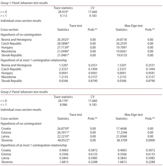
Table 8b. Panel johansen test results and individual cross-section results.
trace test indicates 1 cointegrating eqn(s) at the 0.05 level; * statistically significant; ** mackinnon, haug, and michelis (1999) p-values; Probabilities are computed using asymptotic chi-square distribution.
source: authors.
Group 1: Panel johansen test results
trace statistics cv
r = 0 28.910* 17.660
r < 1 9.113 9.183
individual cross-section results
trace test max-Eign test cross-section statistics Prob.** statistics Prob.** hypothesis of no cointegration
Bosnia and herzegovia 26.3925* 0.00 24.8718 0.00 czech Republic 28.5896* 0.00 26.2559 0.00
hungary 27.7139* 0.00 19.7097 0.00
macedonia 21.0496* 0.00 19.8361 0.00
slovak Republic 21.0481* 0.00 19.0135 0.00 hypothesis of at most 1 cointegration relationship
Bosnia and herzegovia 1.5207 0.2551 1.5207 0.2551 czech Republic 2.3337 0.1494 2.3337 0.1494
hungary 0.0041 0.9581 0.0041 0.9581
macedonia 1.2135 0.3157 1.2135 0.3157 slovak Republic 0.0346 0.8790 0.0346 0.8790
Group 2: Panel johansen test results
trace statistics cv
r = 0 28.170* 17.660
r < 1 8.986 9.183
individual cross-section results
trace test max-Eign test cross-section statistics Prob.** statistics Prob.** hypothesis of no cointegration
croatia 26.8759* 0.00 17.4696 0.00
Estonia 26.5911* 0.00 17.2346 0.00
Latvia 22.2210* 0.00 21.8368 0.00
slovenia 40.0522* 0.00 38.3709 0.0000 hypothesis of at most 1 cointegration relationship
croatia 0.4063 0.5872 0.4063 0.5872 Estonia 0.3566 0.6133 0.3566 0.6133 Latvia 0.3843 0.5985 0.3843 0.5985 slovenia 1.6813 0.2288 1.6813 0.2288
at the 1% level, support the cointegration relationships of economic growth and biomass consumption found in the Johansen test.
Pedroni results verify the cointegration relationship between the analysed variables. On the other hand, Table 8b shows the individual cross-section results in Groups 1 and 2. Thus, the evidence suggests that, in both panel datasets and in the individual cross-sections, there is a long-run equilibrium relationship between biomass energy consumption and economic growth.
For Group 2, Table 8b shows individual cross-section results for the panel Johansen test. Thus, the evidence suggests that, in both panel datasets and in individual cross-sections, there is a long-run equilibrium relationship between biomass energy consumption and economic growth.
4.2.3. F.M.O.L.S. estimates
F.M.O.L.S. results indicate the existence of a strong relationship between economic growth and biomass energy consumption in Table 9. Accordingly, a 1% increase in the G.D.P. enhances biomass energy consumption by 1.013% in Group 1, but 0.75698% for Group 2. In this regard, biomass consumption should be explicated as normal goods.
4.2.4. Panel Granger causality test
Table 10 shows the results of error correction estimates, the short-run and long-run results and Granger causality for the analysed panels denoted as Groups 1 and 2. For group 2 countries and Bulgaria, E.C.M. results show that the system turns back to its long-run equilibrium in ~ 2 years after an economic shock, similarly with A.R.D.L. result for Bulgaria (−0.5073), which is shown in Table 5. E.C.T. is −0.441 in Group 1 and −0.504 in Group 2 and speed of adjustment is high, so, after a shock, the system turns back to its long-run equilibrium level in ~ 2 years.
Table 9. F.m.o.L.s. results.
source: authors. F.M.O.L.S. results c (t-stat) y (t-stat) R2 Group 1 −0.5808 (−4.096) 1.0130 (3.010) 0.701 Group 2 0.8965 (1.869) 0.7570 (2.259) 0.785
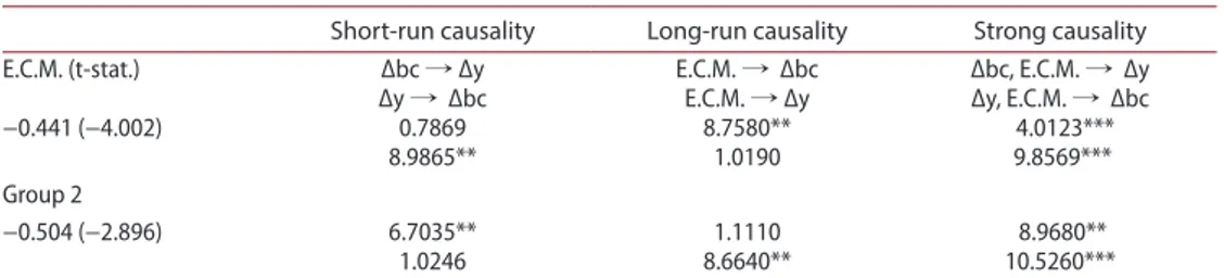
Table 10. Results of Granger causality.
note: the values in parentheses are t-values. significance levels: * p < 0.05; ** p < 0.01; and *** p < 0.001. For the co-joint test, we used the Wald-test (χ2). in this table, the symbol → shows the direction of causality.
source: authors. Group 1
Short-run causality Long-run causality Strong causality E.c.m. (t-stat.) Δbc → Δy E.c.m. → Δbc Δbc, E.c.m. → Δy Δy → Δbc E.c.m. → Δy Δy, E.c.m. → Δbc −0.441 (−4.002) 0.7869
8.9865** 8.7580** 1.0190 4.0123*** 9.8569*** Group 2
−0.504 (−2.896) 6.7035** 1.1110 8.9680** 1.0246 8.6640** 10.5260***
For Groups 1 and 2, the calculated Chi-square statistics are above the critical value with 2 degrees of freedom, suggesting a rejection of the null hypothesis of no Granger causality between biomass consumption and economic growth at 5% significance level. It was deter-mined from the evidence to reject the null hypothesis for the one-direction causal relation-ship between variables for Groups 1 and 2. In Group 2, there is unidirectional causality from biomass consumption to economic growth as a result of the short- and long-run Granger causality supporting the growth hypothesis. The results of the growth hypothesis are similar to the results obtained for Bulgaria and Romania by Granger Causality method. However, in strong causality, there is evidence to reject the null hypothesis for bidirectional causality between biomass consumption and economic growth. In Group 1, there is unidirectional causality from economic growth to biomass consumption as a result of short- and long-run Granger causality, supporting the conservation hypothesis. Similarly, in strong causality there is evidence to reject the null hypothesis for bidirectional causality between biomass consumption and economic growth.
Strong Granger causality results in Groups 1 and 2 show the importance of biomass energy consumption for the two groups. Energy conservation policies may decrease eco-nomic growth performance and the changes in ecoeco-nomic growth may decrease energy consumption. An energy policy focused on diminishing biomass energy consumption neg-atively affects the countries’ economic growth. F.M.O.L.S. results denote biomass energy as normal good in Group 2. The A.R.D.L. results support the feedback hypothesis in the context of strong causality results. These findings are supported by Bildirici and Ozaksoy’s (2014) results for Hungary, Bulgaria, Romania, Slovenia, Croatia and Slovakia.
5. Conclusion
This paper focuses on investigation of the relationship between biomass energy consumption and economic growth, which was tested by time series (A.R.D.L. and Granger Causality) and Panel methods (Panel Cointegration: Pedroni-Panel Johansen test and Panel Granger models). A.R.D.L. and Granger Causality methods were applied for Albania, Romania and Bulgaria. The short-run causality results indicate evidence of uni-directional causality from economic growth to biomass energy consumption for Albania. However, for Bulgaria and Romania, the causality results show evidence of uni-directional causality from biomass energy consumption to economic growth, which promotes the growth hypothesis. The feedback hypothesis is found in strong causality results for all of the analysed countries.
A second method was applied to Bosnia and Herzegovina, Bulgaria, Croatia, Czech Republic, Estonia, Hungary, Latvia, Macedonia, Romania, Slovak Republic and Slovenia. According to Panel Granger causality test results, both in the short-run and long-run, there is evidence of uni-directional causality from economic growth to biomass energy consumption in Bosnia and Herzegovina, Czech Republic, Hungary, Macedonia and Slovak Republic. These findings support the conservation hypothesis for these countries. Short-run and long-Short-run causality test results prove uni-directional causality from biomass energy consumption to economic growth, which supports the growth hypothesis not only for Croatia, Slovenia, Estonia and Latvia, but also for Bulgaria and Romania. However, strong causality test results signal bidirectional causality between biomass energy consumption and economic growth, which emphasises the feedback hypothesis in all these countries.
Regarding our empirical results, for the analysed countries, development of the biomass energy infrastructure and encouragement of biomass energy consumption are important energy policy tools as they promote economic growth, while also being affected by it. In this context, biomass energy consumption should be enhanced for these countries. Biomass energy consumption has direct and indirect effects on economic growth. If energy needs are obtained from biomass energy resources, energy dependence on fossil fuels from exporter countries will decrease. On the one hand, modern biomass energy is a way of decreasing foreign oil dependency while, on the other hand, modern biomass energy can benefit rural employment.
As a result, transition countries must encourage biomass energy consumption to enable sustainable economic growth and development. Furthermore, environmental protection necessarily meets part of a country’s needs, promotes energy security and reduces poverty.
Disclosure statement
No potential conflict of interest was reported by the authors.
References
Ali, H. S., Law, S. H., Yusop, Z., & Chin, L. (2016). Dynamic implication of biomass energy
consumption on economic growth in Sub-Saharan Africa: Evidence from panel data analysis. GeoJournal1. doi:10.1007/s10708-016-9698-y
Al-mulali, U., Fereidouni, H. G., Lee, J. Y., & Sab, C. N. B. C. (2013). Examining the bi-directional
long run relationship between renewable energy consumption and GDP growth. Renewable and Sustainable Energy Reviews, 22, 209–222.
Apergis, N., & Payne, J. E. (2010a). Renewable energy consumption and growth in Eurasia. Energy
Economics, 32, 1392–1397.
Apergis, N., & Payne, J. E. (2010b). Renewable energy consumption and economic growth: Evidence
from a panel of OECD countries. Energy Policy, 38, 656–660.
Apergis, N., & Payne, J. E. (2011a). The renewable energy consumption–growth nexus in Central
America. Applied Energy, 88, 343–347.
Apergis, N., & Payne, J. E. (2011b). Renewable and non-renewable electricity consumption–growth
nexus: Evidence from emerging market economies. Applied Energy, 88, 5226–5230.
Aslan, A. (2016). The causal relationship between biomass energy use and economic growth in the
United States. Renewable and Sustainable Energy Reviews, 57, 362–366.
Balat, M. (2005). Use of biomass sources for energy in Turkey and a view to biomass potential.
Biomass and Bioenergy, 29, 32–41.
Bildirici, M. (2004a). Political instability and growth: An econometric analysis of Turkey, Mexico,
Argentina and Brazil, 1985–2004. Applied Econometrics and International Development, 4(4), 5–26.
Bildirici, M. (2004b). Real cost of employment an Turkish labor market: A panel cointegration tests
approach. International Journal of Applied Econometrics and Quantitative Studies, 1(2), 95–120.
Bildirici, M. (2012). The relationship between economic growth and energy consumption. Journal
of Renewable and Sustainable Energy, 4(2), 5. doi:10.1063/1.3699617
Bildirici, M. (2013). Economic growth and biomass energy. Biomass and Bioenergy, 50, 19–24.
doi:10.1016/j.biombioe.2012.09.055.2012
Bildirici, M. (2014). Relationship between biomass energy and economic growth in transition
countries: Panel ARDL approach. GCB Bioenergy, 6, 717–726. doi:10.1111/gcbb.12092
Bildirici, M. (2016). Biomass energy consumption and economic growth: ARDL analysis. Energy
Bildirici, M., & Bohur, E. (2014). Design and economic growth: Panel cointegraiton and causality analysis. In 4th International Conference on Leadership, Technology and Innovation Management. Yıldız Technical University.
Bildirici, M., & Ersin, Ö. Ö. (2015). An ınvestigation of the relationship between the biomass
energy consumption, economic growth and oil prices. In Procedia Social and Behavioral Sciences. Proceedings of the 4th International Conference on Leadership, Technology, Innovation and Business Management (ICLTIBM-2014).
Bildirici, M., Ersin, O. O., & Kokdener, M. (2011). Genetic structure, consanguineous marriages and
economic development: Panel cointegration and panel cointegration neural network analyses. Expert Systems with Applications, 38(5), 6153–6163. doi:10.1016/j.eswa.2010.11.056.
Bildirici, M., & Kayıkcı, F. (2012). Economic growth and electricity consumption in emerging
countries of Europa: An ARDL analysis. Economic Research, 25(3), 538–558.
Bildirici, M., & Ozaksoy, F. (2013). The relationship between economic growth and biomass energy
consumption in some European countries. Journal of Renewable and Sustainable Energy, 5(2),
5–13. doi:10.1063/1.4802944
Bildirici, M., & Ozaksoy, F. (2014). Biomass energy consumption, economic growth in transition
countries. In International Energy Technologies Conference, ENTECH’14. Yildiz Technical University.
Bilgili, F., & Ozturk, I. (2015). Biomass energy and economic growth nexus in G7 countries: Evidence
from dynamic panel data. Renewable and Sustainable Energy Reviews, 49, 132–138.
Engle, R. F., & Granger, C. W. J. (1987). Co-integration and error correction: Representation,
estimation, and testing. Econometrica, 55, 251–276.
Johansen, S. (1991). Estimation and hypothesis testing of cointegration vectors in gaussian vector
autoregressive models. Econometrica, 59(6), 1551–1580.
Johansen, S. (1988). Statistical analysis of cointegration vectors. Journal of Economic Dynamics and
Control, 12, 231–254.
Johansen, S., & Juselius, K. (1990). Maximum likelihood estimation and ınference on cointegration:
With applications to the demand for money. Oxford Bulletin of Economics and Statistics, 52, 169– 210.
Larsson, R., & Lyhagen, J. (2007). Inference in panel cointegration models with long panels. Journal
of Business & Economic Statistics, 25, 473–483.
Larrson, R., Lyhagen, J., & Lothgren, M. (2001). Likelihood-based cointegration tests in heterogeneous
panels. Econometrics Journal, 4(1), 109–142.
Lee, C. C., & Chang, C. C. (2008). Energy consumption and economic growth in Asian economies:
A more comprehensive analysis using panel data. Resource and Energy Economics, 30(1), 50–65.
MacKinnon, J. G., Haug, A. A., & Michelis, L. (1999). Numerical distribution functions of likelihood
ratio tests for cointegration. Journal of Applied Econometrics, 14, 563–577.
Menegaki, A. N. (2011). Growth and renewable energy in Europe: A random effect model with
evidence for neutrality hypothesis. Energy Economics, 33, 257–263.
Menyah, K., & Wolde-Rufael, Y. (2010). CO2 emissions, nuclear energy, renewable energy and
economic growth in the US. Energy Policy, 38, 2911–2915.
Narayan, P. K. (2005). The saving and investment nexus for China: Evidence from cointegration tests.
Applied Economics, 37, 1979–1990.
Ocal, O., & Aslan, A. (2013). Renewable energy consumption–economic growth nexus in Turkey.
Renewable and Sustainable Energy Reviews, 28, 494–499.
Öztürk, F., & Bilgili, İ. (2015). Economic growth and biomass consumption nexus: Dynamic panel
analysis for Sub-Sahara African countries. Applied Energy, 137, 110–116.
Payne, J. E. (2011). On biomass energy consumption and real output in the US. Energy Sources, Part
B: Economics, Planning, and Policy, 6(1), 47–52.
Pedroni, P. (1999). Critical values for cointegration tests in heterogeneous panels with multiple
regressors. Oxford Bulletin of Economics and Statistics, 61, 653–670.
Pedroni, P. P. (2004). Panel cointegration: Asymptotic and finite sample properties of pooled time
series tests, with an application to the PPP Hypothesis. Indiana University Working Papers in Economics, 597–625.
Pesaran, M. H., & Shin, Y. (1999). An autoregressive distributed lag modelling approach to cointegration analysis. In S. Strom, (Ed.), Econometrics and Economic Theory in the 20th Century: The Ragnar Frisch Centennial Symposium. Cambridge: Cambridge University Press.
Pesaran, M. H., Shin, Y., & Smith, R. J. (2001). Bounds testing approaches to the analysis of level
relationships. Journal of Applied Econometrics, 16, 289–326.
Phillips, P. C. B., & Hansen, B. E. (1990). Statistical inference in instrumental variable regression with
I(1) processes. Review of Economic Studies, 57, 99–125.
Purna, C. P., & Pravakar, S. (2007). Export-led growth in South Asia: A Panel cointegration analysis.
International Economic Journal, 21(2), 155–175.
Sardorsky, P. (2009a). Renewable energy consumption and income in emerging economies. Energy
Policy, 37, 4021–4028.
Sardosky, P. (2009b). Renewable energy consumption, CO2 emissions and oil prices in the G7
countries. Energy Economics, 31, 456–462.
Shahbaz, M., Rasool, G., Ahmed, K., & Mahalik, M. K. (2016). Considering the effect of biomass
energy consumption on economic growth: Fresh evidence from BRICS region. Renewable and Sustainable Energy Reviews, 60, 1442–1450.