IS THE TOURISM-LED GROWTH HYPOTHESIS (TLGH)
VALID FOR TURKEY?
TURİZME DAYALI BÜYÜME HİPOTEZİ TÜRKİYE İÇİN GEÇERLİ Mİ?
Harun TERZİ
Karadeniz Teknik Üniversitesi İİBF İktisat Bölümü İktisat Politikası Anabilim Dalı [email protected]
ABSTRACT: This study focuses on the causality relationship between international tourism revenue and economic growth in the Turkish economy during the period 1963-2013. Yearly time series data were obtained from the World Data Indicators and the Turkish Statistical Institute. Three different methodologies were employed to test the causality: pairwise Granger causality, unrestricted VAR and Toda-Yamamoto VAR analysis. All tests yielded strong evidence for unidirectional positive significant causality running from tourism revenue to economic growth. Additionally, IR and VD analyses also showed that the two variables affect each other. The findings of this study support the view that tourism-led growth hypothesis is valid for the Turkish economy. Key Words: Tourism Revenue; Economic Growth; Causality; VAR Analysis; Turkey
JEL Classifications C32; F14; L83
ÖZET: Bu çalışmada uluslararası turizm gelirleri ile ekonomik büyüme arasındaki nedensellik ilişkisi 1963-2013 dönemi Türkiye ekonomisi için incelenmiştir. Araştırmada kullanılan yıllık zaman serileri Dünya Kalkınma Göstergeleri’nden (WDI) ve Türkiye İstatistik Kurumu’ndan (TÜİK) derlenmiştir. Nedenselliği test etmek amacıyla bu çalışmada standart Granger nedensellik, kısıtsız ve Toda Yamamoto VAR nedensellik gibi üç farklı nedensellik analizi kullanılmıştır. Tüm testler nedenselliğin güçlü bir şekilde turizm gelirlerinden ekonomik büyümeye doğru, pozitif ve tek yönlü olduğunu; ayrıca ET ve VA analizleri iki değişkenin birbirlerini karşılıklı olarak etkilediklerini göstermektedir. Bu çalışmanın bulguları, turizme dayalı büyüme hipotezinin Türkiye için geçerli olduğunu göstermektedir.
Anahtar Kelimeler: Turizm Geliri; Ekonomik Büyüme; Nedensellik; VAR Analizi; Türkiye
1. Introduction
The relationship between international tourism and economic growth has become a popular research topic, particularly in developing countries. There are three different hypotheses regarding the causal relationship between tourism and economic growth in the literature: 1) The tourism-led growth hypothesis; 2) The growth-led tourism hypothesis, and 3) The growth-led tourism and tourism-led growth hypothesis. Tourism and economic growth have a mutual effect on each other. The common view is that tourism revenues can increase income, employment and investment in the tourism sector. Tourism income is an important determinant of economic growth, and therefore can stimulate overall economic performance. It is a general view, especially in developing countries, that tourism has the potential to speed up economic growth and become an engine for growth in both short and long-run. This common view is known in the literature as the Tourism-Led Growth Hypothesis (TLGH). According
to the TLGH, more resources should be allocated to the tourism industry relative to other sectors. Analysis of the validity of the TLGH in the case of Turkey could prove useful for similar analyses of other developing countries.
The Turkish tourism industry has grown rapidly. In particular, the industry has boomed since 2004 and, in order to increase the tourism potential of the country, the government has supported numerous projects by both local and international investors to attract tourists from all over the world. Between 2002 and 2013, international tourist arrivals in Turkey increased substantially, from 12.8 million to 39.7 million, making Turkey a top 10 destination in the world for international tourists. In 2014 more than 30 million tourists visited Turkey, compared to 28 million over the same period in 2013, according to the Tourism Ministry. Turkey ranked as the sixth most popular tourist destination in the world and fourth in Europe, according to the UNWTO World Tourism Barometer. Turkey’s total tourism income was $32 billion in 2013 and Business Monitor International forecasts revenues to exceed $35 billion by 2017. In this study, section 2 presents the literature review, section 3 describes the model, variables and econometric methodology employed, section 4 presents the empirical causality findings, and finally section 5 provides a summary with concluding remarks.
2. Literature Review
Numerous empirical country studies in the literature have shown that the validity of TLGH is controversial and inconclusive. A significant amount of research has been conducted in developing/emerging economies to establish this hypothesis. A comparative survey of empirical results from causality tests of tourism activity and economic growth in Turkey and selected countries is listed in the article by Milanovic and Stamenkovic (2012). The results of various studies for the Turkish economy can be summarized as follows: Yıldırım-Öcal (2004) examined the effects of tourism revenues for economic growth for the period 1962-2002, in a VAR framework. Their findings indicated that even though there are growth-promoting effects on tourism revenues in the long-run, there is no short-run relationship between tourism and economic growth. Kasman-Kasman (2004) investigated the long-term relationship between economic growth and tourism for the period 1963-2002 by using Johansen’s multivariate procedure and Pesaran et al.’s (2001) bounds test procedure. They found that tourism unilaterally affects economic growth. Therefore, the results confirm the validity of the tourism-led growth hypothesis. Ongan-Demiröz (2005) investigated the impact of international tourism receipts on long-term economic growth over the period of 1980:q1-2004:q2 by using the Johansen cointegration test and VECM. They found that there is a bidirectional causality between international tourism and economic growth both in the short-run and long-run. Gündüz-Hatemi (2005) empirically supported the TLG hypothesis for Turkey by making use of leveraged bootstrap causality tests for the period 1963-2000. Yavuz (2006) suggested that there was no causality between tourism receipts and economic growth by using the standard Granger and Toda-Yamamoto (1995) causality tests over the period 1992:q1-2004:q4. Özdemir-Öksüzler (2006) found a one-way causality relationship from tourism revenue to GDP, both in the short and long-run for the 1963-2003 period with the Johansen co-integration test and VECM. Kızılgöl-Erbaykal (2008) investigated the causal relationship between tourism revenues and economic growth by using quarterly data for the 1992:q1-2006:q2 periods with the Toda-Yamamoto causality method, and found that there is a unidirectional causality running from economic growth to tourism revenues. Kaplan-Çelik (2008) examined the relationship between tourism expansion
and economic performance over the period 1963-2006. Empirical analysis carried out by the VAR procedure indicated the presence of one cointegrating vector between real output, real tourism receipts and real effective exchange rate and also that tourism has a long-run effect on output. In addition, test results showed the presence of one-directional causality indicating that tourism and the exchange rate cause output. Çetintaş -Bektaş (2008) investigated short and long-term relationships and causality between tourism and economic growth by using the ARDL method for the period 1964-2006. They found that tourism is an important factor of economic growth in the long-term, and Granger causality runs from tourism to economic growth. The long- term relationship between the two variables and the unidirectional causality from economic growth to tourism revenues confirm that, in the long-term, the tourism-led growth hypothesis is valid for Turkey.
Zortuk (2009) examined the contribution of the tourism sector to economic growth by using data from 1990:q1 to 2008:q3, and showed the existence of a uni-directional causality running from tourism development to economic development. Öztürk-Acaravci (2009) investigated the long-run relationship between real GDP and international tourism during the time period 19872007 by using different methods -VEC, the ARDL bound and Johansen cointegration test - and showed that there is no unique long-term or equilibrium relationship between real GDP and international tourism. Katırcıoğlu (2009) examined the long-run impact of the total number of international tourists visiting and booking accommodating on real GNP and real exchange rates during the period from 1960 to 2006 by using unit roots, bounds and Johansen tests. His results suggest that the TLGH cannot be inferred for Turkey since tests do not confirm long-run relations between the variables.
Polat-Günay (2012) studied the joint effect of exports and tourism receipts on economic growth by cointegration and causality analysis based on VECM, by using annual data of export receipts, tourism receipts and GDP for the period 1969-2009. They found evidence for TLGH in that there is a long-run relationship between tourism receipts and economic growth, and there is only one-way causality running from tourism receipts to economic growth. Yurtseven (2012) found that tourism earnings are essential to increase real GDP in Turkey, by using a multivariate VAR model, including real export volume and real exchange rates, on quarterly data from 1980 to 2011. He found that the relationship seemed to be uni-directional, and that tourism earnings appeared to be caused by real GDP growth. Arslantürk-Atan (2012) analyzed the relationship between growth, foreign exchange and tourism receipts by applying the cointegration and Granger causality tests for the period 1987-2009. They showed that there is a causal relationship running from tourism incomes to economic growth, which supports the premise that international tourism helps to increase employment and economic growth. The present study aims to determine the role of international tourism revenue in the Turkish economy, and particularly the effects of tourism revenue on real economic growth, with regard to the validity of the TLGH for Turkey. Since the beginning of the 2000s, there have been extensive empirical studies on the causality relation between tourism activity and economic growth. Some of these studies have been summarized in Table 1.
Most of the empirical results reached the conclusion that the TLGH is valid for Turkey. However, a small number of studies found no causality, reverse causality or bi-directional causality between the two variables. This study contributes to the
literature by applying three different methodologies of causality analysis- pairwise, standard VAR and Toda-Yamamoto VAR Granger causality tests- and compares their results before offering suggestions about how the issue may be addressed in future.
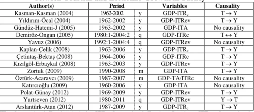
Table 1. Evidence from Empirical Results on Causality between Tourism and Economic Growth in Turkey
Author(s) Period Variables Causality
Kasman-Kasman (2004) 1962-2002 y GDP-ITRc T Y
Yıldırım-Öcal (2004) 1962-2002 y GDP-ITRev T Y Gündüz-Hatemi-J (2005) 1963-2002 y GDP-ITA No causality
Demiröz-Ongan (2005) 1980:1-2004:2 q GDP-ITRc T Y Yavuz (2006) 1992:1-2004:4 q GDP-ITRev No causality Kaplan-Çelik (2008) 1963-2006 y GDP-ITRc T Y
Çetintaş-Bektaş (2008) 1964-2006 y GDP-ITRc T Y Kızılgöl-Erbaykal (2008) 1963-2003 y GDP-ITRev T Y Zortuk (2009) 1990-2008 m GDP-ITA T Y Öztürk-Acaravcı (2009) 1987-2007 m GDP-TA/ITRc No causality
Katırcıoğlu (2009) 1960-2006 y GDP-ITA No causality Polat-Günay (2012) 1969-2009 y GDP-ITRev T Y
Yurtseven (2012) 1980-2011 q GDP-ITRev Y T Arslantürk-Atan (2012) 1987-2009 y GDP-ITRc T Y ITA: International Tourist Arrivals; ITRc: International Tourism Receipts; ITRev: International
Tourism Revenues; TIT: Total Income of Tourism; y : yea r l y; m: m o n t h ly; q : q u a rt erl y d a t a .
TY denotes causality running from tourism to economic growth; TY denotes causality running
from economic growth to tourism; TY denotes bi-directional causality between tourism development
and economic growth.
3. Model, Variables and Methodology
In equation form, the relationship between tourism revenue (hereafter referred to as T) and the gross domestic product (hereafter referred to as Y) of the Turkish economy can be expressed as follows: Y=f(T), where real Y is the gross domestic product in millions of USD based on 2005 prices, as an indicator which measures total economic growth, and real T is the total tourism revenue in USD based on 2005 prices as an indicator of tourism development. The study uses long and up-to-date annual time-series data (1963-2013), with a total of 42 observations for each variable. Analyses have been carried out by e-views9, jmulti4 and gretl1.9. All variables are in natural
logarithmic terms. Before applying causality analysis in determining the interdependence and dynamic relationships between variables, Augmented Dickey-Fuller (ADF) [Dickey-Dickey-Fuller, (1979); (1981)], Phillips-Perron (PP) [Phillips-Perron, (1988)] and KPSS [Kwiatkowski-Phillips-Schmidt-Shin, (1992)] unit root tests are conducted to determine the order of integration for each variable by SIC criterion. Besides the ADF test, in this study PP and KPSS tests are also employed by the AR spectral OLS detrended estimation method to cross-check the maximum order of integration. As the ADF test may have lower power compared to the stationary near unit root processes, PP and KPSS tests are also utilized as complements. There are multiple ways to perform the Granger causality tests between two variables. The empirical analysis in this study is carried out by using three alternative Granger causality models -pairwise, standard/unrestricted, and Toda-Yamamoto (TY) Granger causality tests- to capture the linear interdependencies between time series. The VAR model made popular by Sims (1980) is one of the most flexible and the easiest to use for describing the dynamic behavior of economic time series. CUSUM, CUSUMQ tests, impulse-response (IR) and variance decompositions analyses (VD) have also been applied to all three VAR models, and results are found to be conclusive.
Therefore, in order to save space, only the test outcomes from the TY VAR (4) model have been presented in this study.
Granger (1969) proposed a simple model for a causality test to be used for the study of the mutual influence within two economic variables, such as tourism revenue and national income, based on the equations below:
t 1 j t j p 1 j i t i p 1 i t
Y
T
u
Y
(1) t 2 j t j q 1 j i t i q 1 i tT
Y
u
T
(2)Given two stationary time series variables T and Y, T is said to Granger causes Y if Y can be better predicted by using the lagged values of both T and Y. According to Granger and Newbold (1974) variables have to be covariance stationary in Granger to avoid spurious relations. In equations 1 and 2, , , , , and parameters of the model u1t and u2t are assumed to be uncorrelated error terms. Based on the OLS
coefficients for equations 1 and 2, two different hypotheses can be tested as follows: 1) h0: j=0 for all j and 2) h0: j=0 for all j. In the alternative hypothesis that j≠0
(j≠0) for at least some j’s if any or all of 1, …, p (1, …, q) are statistically
significant T Granger causes Y (Y Granger causes T). The pairwise Granger causality test is easy to apply, but it is sensitive to lag selection and it has some limitations. In the unrestricted VAR Granger causality/block exogeneity Wald model proposed by Sargent (1976), Y and T are stationary variables, c1 and c2 are the intercept terms, a11,
a12, a21 and a22 are the coefficients of the endogen variables and u1t and u2t are the
stochastic error terms. The VAR Granger causality test is used to determine the short-run causality between T and Y, and also the direction of causality. In a two variable VAR of order 3, this test looks at whether the lags of any variable Granger cause to other variables in the following equation (3):
[Yt Tt] = [ 𝑎111 𝑎121 𝑎211 𝑎221 ] [ Yt−1 Tt−1] + [ 𝑎112 𝑎122 𝑎212 𝑎222] [ Yt−2 Tt−2] + [ 𝑎113 𝑎123 𝑎213 𝑎223] [ Yt−3 Tt−3] + [ c1 c2] + [ u1t u2t] (3)
The Wald test is used to test whether the lagged values of T (Y) in the Y (T) equation are simultaneously different than zero. If h0: 𝑎121 =𝑎122 =𝑎123 =0 (h0: 𝑎211 =𝑎212 =𝑎213 =0)
hypothesis is rejected, then T Granger causes Y (Y Granger causes T). Rejection of the null hypotheses implies that there is a bidirectional causality between Y and T. Toda-Yamamoto (TY) (1995) proposed a causality analysis to avoid the problems related to the standard Granger causality analysis. The TY method is a different kind of the standard VAR model in the levels of the variables (rather than the first differences, as is the case with the Granger causality tests) thereby minimizing the risks associated with the possibility of wrongly identifying the order of integration of the series. The basic idea of this approach is to artificially augment the optimal VAR order, k, by the maximal order of integration, say dmax. Then, a (k+dmax)th order of VAR is estimated
and the coefficients of the last lagged dmax vector are ignored (Wolde-Rufael, 2005). The
application of the TY (1995) procedure ensures that the usual test statistic for the Granger causality has the standard asymptotic distribution where valid inference can be made. To undertake the TY (1995) version of the Granger non-causality test, the TY
model is represented in the VAR system which follows below. The study uses bivariate VAR(k+dmax) comprised of T and Y, following Yamada (1998):
t 1 i t i x k 1 k i i t i k 1 i i t i k 1 k i i t i k 1 i t
T
T
Y
Y
u
T
dmax
dma
(4) t 2 i t i ax k 1 k i i t i k 1 i i t i x k 1 k i i t i k 1 i tY
Y
T
T
u
Y
dma
dm
(5)where , , , , , , , , and are parameters of the model and dmax is the
maximum order of integration suspected to occur in the system; u1t~N(0, Σu1) and
u2t~N(0, Σu2) are the residuals of the model and Σu1t and Σu2t the covariance matrices
of u1t and u2t, respectively. From equation (4), Granger causality from Y to T implies
h0: 10, (i=1, 2,…,k) ; and similarly in equation (5), T Granger causes Y, if h0: 10,
(i=1, 2,…,k). There are two steps to implement the procedure: 1) determination of the lag length (k), and 2) selecting of the maximum order of integration (dmax) for the
variables in the model.
Lag length selection criterias such as the Akaike Information Criterion (AIC) and the Schwarz Information Criterion (SIC) can be used to determine the appropriate lag order of the VAR. The main reason for conducting unit root tests is to determine the extra lags to be added to the vector autoregressive (VAR) model for the TY test. It is well known that residuals from a VAR model are generally correlated and changing the order of the variables could greatly change the results of the impulse-response (IR) analysis. IR indicates the dynamic effects of a shock of one variable on the other one, as well as on the variable itself. IR analysis is helpful to see the direction of the effect, positive/negative, and the strength of the effect of each variable in the VAR model, whether or not T (Y) has a positive/negative effect on Y (T), and whether or not the impact of T on Y is stronger than that of Y on T. To find the answer, it is necessary to analyze theIR function. The IR function measures the effect of shocks on the future values of T and Y in a dynamic VAR system.
The variance decomposition (VD) allows a better understanding of the double causality between the variables. The VD shows the contribution of each source of innovation to the variance of k-year ahead forecast error for each of the variables included in the system. In other words, variance decompositions show how much of the forecast error variance for each endogenous variable can be explained by each disturbance. As this decomposition is not unique, given the results of these causality tests, the variables are ordered by considering the cases where the associated F-statistics were higher. This calculation is achieved by orthogonalization of the innovations by using the Cholesky decomposition method. This decomposition depends on the order in which the variables enter the VAR system.
4. Empirical Findings
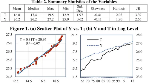
Pearson’s r correlation coefficient (r=0.986), a measure of the strength and direction of the linear relationship between Y and T, is statistically significant as shown by the one-tailed test. There is a significant linear correlation between the two variables. The summary statistics for the variables from 51 observations are presented in Table 2. Median and mean do not differ systematically, therefore variables are symmetric, and p-values of the Jarque-Bera (JB) test, 0.18 for T and 0.27 for Y, show that variables have skewness and kurtosis matching a normal distribution.
Table 2. Summary Statistics of the Variables
Mean Median Max Min Std.
Dev. Skewness Kurtosis JB T 16.8 17.4 19.5 12.9 1.97 -0.41 2.03 3.39 Y 26.2 26.2 27.2 25.0 0.62 -0.11 1.90 2.65
Figure 1. (a) Scatter Plot of Y vs. T; (b) Y and T in Log Level
In Figure 1 (a), the scatter plot of Y vs. T shows positive correlation between the two variables. Of course, correlation does not imply causality, but gives a clue that T and Y might be related and that they move together. Figure 1 (b) shows Y and T variables in log levels over time. Figure 2 shows Y and T variables in the first differences.
Figure 2. Y and T in First Differences
The results are conclusive, as displayed in Tables 3, 4 and 5, and show that all variables are not stationary at level values, and contain unit roots in their levels. However, when the first differences of the variables are taken, they become stationary in all tests. Therefore, it is concluded that each series used in the analysis is integrated as of order one, i.e. I(1). T+C represents the most general model with a drift and trend; C is the model with a drift and without trend.
Table 3. ADF Unit Root Test
Level Data I(0) First Differences I(1)
Model Y p T p Y p T p
C -0.989 0 -1.905 0 -7.150a 0 -5.886 a 1 C+T -3.197 0 -2.083 0 -7.149 a 0 -6.180 a 1
Critical values for model C: 1%: -3.568; 5%: -2.921; for model C+T: 1%: -4.152; 5%: -3.502; p is optimal lag by SIC criteria; a shows rejection of null hypothesis of unit root at the 1% level. MacKinnon (1996) one-sided p-values. Y = 0.31T + 20.95 R² = 0.97 24.8 25.3 25.8 26.3 26.8 27.3 12.5 14.5 16.5 18.5 23.0 24.0 25.0 26.0 27.0 28.0 11.5 13.5 15.5 17.5 19.5 21.5 65 70 75 80 85 90 95 99 5 13 T Y -0.5 0 0.5 1 -0.07 -0.02 0.03 0.08 65 70 75 80 85 90 95 99 5 10 13 Y T
Table 4. PP Unit Root Test
Level Data I(0) First Differences I(1)
Model Y p T p Y p T p
C -1.108 4 -2.088 5 -7.163a 3 -6.462a 2 C+T -3.253 2 -2.046 2 -7.252a 4 -6.867a 6
Critical values for model C: 1%: -3.568; 5%: -2.921; for model C+T: 1%: -4.153; 5%: -3.502; p is bandwidth (Newey-West automatic) using Barlett kernel by SIC criteria; a denotes rejection of null hypothesis of stationary at the 1% level. MacKinnon (1996) one-sided p-values.
Table 5. KPSS Stationarity Test
Level Data I(0) First Differences I(1)
Model Y p T p Y p T p
C 82.69 2 317.85 0 0.087a 0 0.249a 0 C+T 0.734 0 2.124 0 0.035a 0 0.032a 0
Critical values for model C: 1%: 0.739; 5%: 0.463; for model C+T: 1%: 0.216; 5%: 0.146 from Kwiatkowski et al (1992); p is lag length (Spectral OLS-detrended AR) based on SIC criteria; a shows that the variable is stationary at the 1% level.
Table 6. Pairwise Granger Causality Test
h0 /lag 3 5 7 8 9 10 Causality j=0 5.14 (0.00)a 3.81 (0.00)a 3.25 (0.01)a 3.21 (0.01)a 3.01 (0.02)b 2.60 (0.04)b TY* R2 0.28 0.43 0.52 0.58 0.63 0.66 j=0 0.17 (0.91) 0.20 (0.96) 0.40 (0.90) 0.34 (0.94) 0.36 (0.94) 0.45 (0.90) No R2 0.11 0.11 0.23 0.26 0.34 0.40
a andb denote the rejection of the null hypothesis at 1% and 5% significance levels; P values are in parenthesis. Rejection means there is causality. * There are no autocorrelation and heteroscedasticity problems, and also error terms are normally distributed in all distributed- lag models.
Since Y and T have to be stationary, the Granger causality test is applied to the first differences of log variables, because Y and T variables are found to be I(1). The results of pairwise Granger causality for equations (1) and (2) are represented in Table 6, reporting the results corresponding to different regressions. Based on the probability values of the F statistics, T Granger causes Y but Y does not Granger cause T. Thus, it can be argued that past values of T contribute to the prediction of the present value of Y. In the pairwise Granger causality test, there is no evidence of causality with 1 and 2 lags. However, there is a one-way Granger causality from lag 3 to 10, so the results show a unidirectional causality running from T to Y.
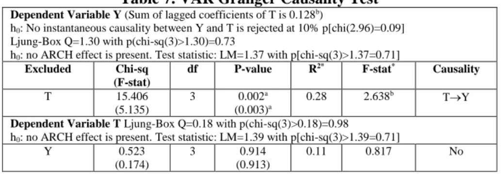
Table 7. VAR Granger Causality Test
Dependent Variable Y (Sum of lagged coefficients of T is 0.128b)
h0: No instantaneous causality between Y and T is rejected at 10% p[chi(2.96)=0.09]
Ljung-Box Q=1.30 with p(chi-sq(3)>1.30)=0.73
h0: no ARCH effect is present. Test statistic: LM=1.37 with p[chi-sq(3)>1.37=0.71] Excluded Chi-sq
(F-stat)
df P-value R2* F-stat* Causality
T 15.406 (5.135) 3 0.002a (0.003)a 0.28 2.638b TY
Dependent Variable T Ljung-Box Q=0.18 with p(chi-sq(3)>0.18)=0.98
h0: no ARCH effect is present. Test statistic: LM=1.39 with p[chi-sq(3)>1.39=0.71]
Y 0.523 (0.174)
3 0.914 (0.913)
0.11 0.817 No
a: significant at 1%, b: significant at 5%, *values of equation Y and T. Modulus of the eigen-values of the reverse characteristic polynomial: |z|=(1.66; 1.66; 2.44; 2.44; 3.19; 4.56). Portmanteau test: LB(11)=38.35, df=32 [0.21]
In the VAR Granger causality model consisting of two stationary variables Y and T, no roots of characteristic polynomial lie outside the unit circle so, VAR satisfies the stability condition. P values of LM stats for lag 1, 2 and 3 are 0.92, 0.64, 0.36; joint p value of JB test is 0.35; P value of Doornik-Hansen test is 0.30. P value of VAR residual heteroscedasticity White test (no cross terms) is 0.55. The residual correlation coefficient is 0.26. Multivariate ARCH-LM test with 3 lags is 33.34 and its p-value (2) is 0.19, p-values (F-stat) of ARCH-LM test with 3 lags for u
1 (u2) is 0.70 (0.71),
and these diagnostic tests give support to the assumptions of the VAR model with regard to white noise residuals. According to the VAR Granger causality test, there is no evidence to contradict the validity of the pairwise Granger causality test in Table 7, indicating that T Granger causes Y at 1% significance level. T affects Y, but Y does not affect T. The Granger causality is running from T to Y.
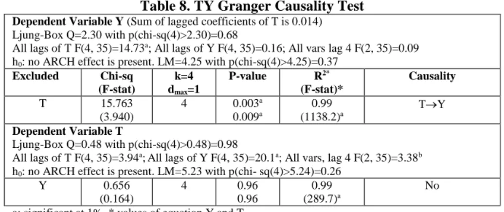
According to unit root tests, the maximum integration number of variables is 1 and the lag length of reduced VAR methodology is 4. Therefore, the VAR (4+1=5) model is estimated and MWALD test is used to examine causality between Y and T. No root lies outside the unit circle and none of the eigenvalues is even close to one, therefore VAR is stable. P values of LM stats for lag 1, 2, 3 and 4 (0.84, 0.15, 0.37, 0.92) are larger than 0.10. Joint p value of JB test is 0.73 and p value of Doornik-Hansen test is 0.95. P value of VAR residual heteroscedasticity White test (no cross terms) is 0.65. The sum of the lagged coefficients in the VAR, excluding the lagged coefficient with the highest order, has a positive sign. The residual correlation coefficient is 0.30. The off-diagonal element of the variance-covariance matrix is 0.002. Diagnostic tests support the contention that the assumptions of the model with regard to white noise residuals are met.
Table 8. TY Granger Causality Test
Dependent Variable Y (Sum of lagged coefficients of T is 0.014)
Ljung-Box Q=2.30 with p(chi-sq(4)>2.30)=0.68
All lags of T F(4, 35)=14.73a; All lags of Y F(4, 35)=0.16; All vars lag 4 F(2, 35)=0.09
h0: no ARCH effect is present. LM=4.25 with p(chi-sq(4)>4.25)=0.37 Excluded Chi-sq (F-stat) k=4 dmax=1 P-value R2* (F-stat)* Causality T 15.763 (3.940) 4 0.003a 0.009a 0.99 (1138.2)a TY Dependent Variable T
Ljung-Box Q=0.48 with p(chi-sq(4)>0.48)=0.98
All lags of T F(4, 35)=3.94a;All lags of Y F(4, 35)=20.1a; All vars, lag 4 F(2, 35)=3.38b
h0: no ARCH effect is present. LM=5.23 with p(chi- sq(4)>5.24)=0.26
Y 0.656 (0.164) 4 0.96 0.96 0.99 (289.7)a No
a: significant at 1%, * values of equation Y and T.
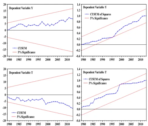
In Table 8, the TY causality test results show null hypothesis, no causality from T to Y can be rejected at the 1% significance level, and virtually at the 5% significance level as well. It means there is a unidirectional causality running from T to Y. As with the CUSUM test, movement outside the critical lines is suggestive of parameter or variance instability. However, the CUSUM and CUSUMQ stability tests, based on the residuals of the TY VAR model, show that the plots of CUSUM stay within the critical 5% bound and the cumulative sum of squares (CUSUMQ) is generally within the 5% significance lines, indicating that the residual variance is mostly stable in Figure 3. In short, two tests show no structural instability in the TY VAR model.
-20 -15 -10 -5 0 5 10 15 20 1980 1985 1990 1995 2000 2005 2010 CUSUM 5% Significance Dependent Variable Y
-0.4 -0.2 0.0 0.2 0.4 0.6 0.8 1.0 1.2 1.4 1980 1985 1990 1995 2000 2005 2010 CUSUM of Squares 5% Significance Dependent Variable Y -20 -15 -10 -5 0 5 10 15 20 1980 1985 1990 1995 2000 2005 2010 CUSUM 5% Significance Dependent Variable T
-0.4 -0.2 0.0 0.2 0.4 0.6 0.8 1.0 1.2 1.4 1980 1985 1990 1995 2000 2005 2010 CUSUM of Squares 5% Significance Dependent Variable T
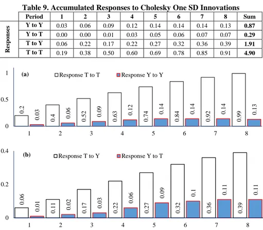
Figure 3. CUSUM and CUSUMQ Statistics for Coefficient Stability of TY VAR Based on the TY VAR model, the impulse-response function traces the effect of a one-time shock to one of the innovations on current and future values of the endogenous variables Y and T. Accumulated responses of Y (T) and T (Y) to the Cholesky one sd. Innovations ± 2 se., for 8 years are illustrated in Figure 4. Table 9 shows the impulse-response functions, which are the response of the two variables to each shock over an eight-year horizon, accumulated orthogonalized impulse-response by the Cholesky ordering: T, Y. The alternative ordering of T and Y is also identical to the initial ordering. In the long-run, an impulse to Y increases Y and T. These are periods when response functions are mostly above the baseline and more than compensate for periods below it. In net terms, Y induces T, and T induces Y. The accumulated effect on T (Y) derived from an impulse on Y (T) is greater than zero, as can be read from Table 9 (df adjusted) and Figure 4.
Figure 4 exhibits the Cholesky asymptotic accumulated impulse-response function of two variables to each shock over an eight-year horizon. It includes 2 figures which are denoted (a) and (b) and illustrate the dynamic cumulative response of each target variable (Y, T) to a one-standard-deviation shock on itself and the other variable. In each figure, the horizontal axis presents the eight years following the shock. The vertical axis measures the yearly impact of the shock on each endogenous variable. In the impulse-response functions of Figure 4a, it shows both variables are positively response by their own impulse. All responses are significant, but the positive effect of T on T is stronger than that of Y on Y.
Table 9. Accumulated Responses to Cholesky One SD Innovations Period 1 2 3 4 5 6 7 8 Sum R esp o n ses Y to Y 0.03 0.06 0.09 0.12 0.14 0.14 0.14 0.13 0.87 Y to T 0.00 0.00 0.01 0.03 0.05 0.06 0.07 0.07 0.29 T to Y 0.06 0.22 0.17 0.22 0.27 0.32 0.36 0.39 1.91 T to T 0.19 0.38 0.50 0.60 0.69 0.78 0.85 0.91 4.90
Figure 4. Accumulated Responses to Generalized One SD Innovations 2se Figure 4b shows that a positive shock to T leads to a positive accumulated response from Y from the first year to the eighth year. Moreover, Y also responds positively to the positive shock of T from the first year to the eighth year. All responses are significant, but the positive response of T to Y is stronger than that of Y to T. Figure 5 exhibits the Cholesky (df adjusted) one sd innovations and responses of T to Y (Y to T), and shows both responses are positive and significant.
Figure 5. Impulse-Responses to Cholesky (df adjusted) One SD Innovations Figure 5 indicates that a positive shock to T leads to a positive response of Y from the third year to the eighth year. Moreover, T also response positively to the positive shock of Y from the first year to the eighth year. All responses are significant, but the
0 -0 .0 0 1 0 .0 0 6 0 .0 2 4 0 .0 2 0 .0 1 4 0 .0 0 9 0 .0 0 2 0 .0 6 1 0 .0 5 4 0 .0 5 2 0 .0 5 4 0 .0 5 1 0 .0 4 9 0 .0 4 1 0 .0 3 2 -0.01 0.01 0.03 0.05 0.07 1 2 3 4 5 6 7 8 Response Y to T Response T to Y 0 .2 0 .4 0.52 0.63 4.70 0.84 0.92 0.99 0 .0 3 0 .0 6 0 .0 9 0 .1 2 0 .1 4 0 .1 4 0 .1 4 0 .1 3 0 0.5 1 1 2 3 4 5 6 7 8
(a) Response T to T Response Y to Y
0 .0 6 0 .1 1 0 .1 7 0 .2 2 0 .2 7 0 .3 2 0 .3 6 0 .3 9 0 .0 1 0 .0 2 0 .0 3 0.06 0.0 9 0 .1 0.1 1 0 .1 1 0 0.2 0.4 1 2 3 4 5 6 7 8 (b) Response T to Y Response Y to T
positive response of T to Y is stronger than that of Y to T. The Granger causality /block exogeneity test shows that Y does not affect T, but Figure 5 shows that a shock to Y has a positive impact on T from the first year to the eighth year.
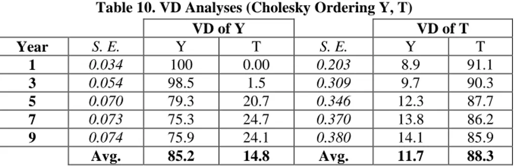
Table 10, comprising eight columns, details the VD for each endogenous variable. The first column lists the time period. The second and fifth columns indicate the standard errors of the sample sets. The third and fourth columns report the variance proportion of the shock to Y. The sixth and seventh columns report the variance proportion of the shock to T.
Table 10. VD Analyses (Cholesky Ordering Y, T)
VD of Y VD of T Year S. E. Y T S. E. Y T 1 0.034 100 0.00 0.203 8.9 91.1 3 0.054 98.5 1.5 0.309 9.7 90.3 5 0.070 79.3 20.7 0.346 12.3 87.7 7 0.073 75.3 24.7 0.370 13.8 86.2 9 0.074 75.9 24.1 0.380 14.1 85.9 Avg. 85.2 14.8 Avg. 11.7 88.3
Variation of Y: The fluctuations of Y are mostly explained by Y shocks, in both the long-run and short-run. Y shock accounts for 100% in the first year. Its proportion in the variance of Y decreases slightly over time and reaches 76% in the ninth year. At period 9, 24% of the variation of Y is explained by past T, and 76% of variation of Y is explained by past Y. The variation of Y can be explained by both past T and past Y in the long-run. Because, in the long-run, T accounts for 15% of the variation of Y on the 9-year average. Variance decomposition showed that 21% of the shocks in Y after five years is due to shocks in T. In the long-run, shock in T is the most important source of variability in Y and is a significant source of increase in Y. T appears to be an important determinant of Y.
Variation of T: T shock accounts for 91% in the first year. Its proportion slightly decreases over time and reaches 86% in the ninth year. At period 9, 86% of the variation of T is explained by past T level, but just 14% of the variation of T is explained by past Y. That means Y shocks are important in part in explaining the level of T, both in the short-run (9%) and in the long-run (14%). In Table 10, variance decomposition shows that shocks in T are very significant source of fluctuations in Y, accounting for 25% of shocks in output after seven years while own shocks accounted for 75%. For T, own shocks accounted for most of the shocks (88%) while Y accounted for only 14%. This result suggests that Y also has a partial effect on T.
5. Conclusion
There are many empirical studies in the literature regarding the tourism-led growth hypothesis (TLGH). In general, findings support the view that tourism promotes economic growth. This paper investigates the role of international tourism on economic growth in Turkey by using alternative VAR causality models - pairwise Granger causality, standard VAR and TY VAR- by using annual data from 1963 to 2013. The pairwise Granger and VAR causality analyses revealed that tourism revenue has a positive significant causality relationship with economic growth, and a unidirectional causality runs from tourism revenue to economic growth.
It is clear from the IR analyses that tourism revenue and economic growth have a positive effect on each other in the long-run. The IR and VD analyses also support causality in the long-run. Findings from the study show that the tourism- led growth hypothesis is valid in Turkey for the period 1963 to 2013. Accordingly, tourism revenue has an important effect on economic growth. In contrast to the findings of Gündüz-Hatemi (2005), Yavuz (2006), Öztürk-Acaravcı (2009) and Katırcıoğlu (2009), this study supports the findings of Kasman-Kasman (2004), Yıldırım-Öcal (2004), Kaplan-Çelik (2008), Çetintaş-Bektaş (2008), Kızılgöl-Erbaykal (2008), Zortuk (2009), Polat-Günay (2012), Yurtseven (2012) and Arslantürk-Atan (2012). This study implies that tourism is essential to boost economic growth in Turkey, and TLGH is valid for the Turkish economy. Therefore, it suggests that government should encourage investment in the tourism sector in order to improve economic growth, as variation in tourism revenue can be seen as a leading indicator of fluctuations in national income.
The causality result of this study based on two variables. However, without considering the effect of other major variables, model is subject to possible specification bias, and causality tests are sensitive to the specification of the model and lag selection procedure. Therefore, further research could be based on alternative, multi variable models in order to find the way of causality and impact of tourism on national income.
6. References
ARSLANTÜRK, Y., ATAN, S. (2012). Dynamic relation between economic growth, foreign exchange and tourism incomes: an econometric perspective on Turkey. Journal of Business, Economics and Finance, 1 (1), pp.30-37.
ÇETİNTAŞ, H., BEKTAŞ, Ç. (2008). Türkiye’de turizm ve ekonomik büyüme arasındaki kısa ve uzun dönemli ilişkiler. Anatolia: Turizm Araştırmaları Dergisi, 19 (1), pp.37-44. DEMİRÖZ, D., ONGAN, S. (2005). The contribution of tourism to the long-run Turkish
economic growth. Ekonomicky Casopis, 9 (1), pp.880-894.
DICKEY, D. A., FULLER, W. A. (1979). Distribution of the estimators for autoregressive time series with a unit root. Journal of the American Statistical Association, 74, pp.427-431.
DICKEY, D. A., FULLER, W. A. (1981). Likelihood ratio statistics for autoregressive time series with a unit root. Econometrica, 49, pp.1057-1072.
ENDERS, W. (2014). Applied econometric time series. 4th edition, New York: Wiley GRANGER, C. W. J. (1969). Investigating causal relations by econometric models and cross
spectral methods. Econometrica, 37, pp.424-438.
GRANGER, C. W. J., NEWBOLD, P. (1974). Spurious regressions in econometrics. Journal of Econometrics, 2, pp.111-120.
GÜNDÜZ, L., HATEMI, J. A. (2005). Is the tourism-led growth hypothesis valid for Turkey? Applied Economics Letters, 12 (8), pp.499-504.
KAPLAN, M., ÇELIK, T. (2008). The impact of tourism on economic performance: the case of Turkey. The International Journal of Applied Economics and Finance, 2, pp.13-18. KASMAN, K, S., KASMAN, A. (2004). Turizm gelirleri ve ekonomik büyüme arasındaki
eş-bütünleşme ve nedensellik ilişkisi. İktisat, İsletme ve Finans Dergisi, 19 (7), pp.122-131. KATIRCIOĞLU, S. T. (2009). Revisiting the tourism-led-growth hypothesis for Turkey using
the bounds test and Johansen approach for cointegration. Tourism Management, 30 (1), pp.17-20.
KIZILGÖL, Ö., ERBAYKAL, E. (2008). Türkiye’de turizm gelirleri ile ekonomik büyüme ilişkisi: bir nedensellik analizi. SDÜ İİBF Dergisi, 13 (2), pp.351-360.
KWIATKOWSKI, D., PHILLIPS, P. C. B., SCHMIDT, P., SHIN, Y. (1992). Testing the null hypothesis of stationarity against the alternative of a unit root: how sure are we that economic time series have a unit root? Journal of Econometrics, 54, pp.159-178. MILANOVIC, M., STAMENKOVIC, M. (2012). Causality between tourism and economic
growth: a case study of Serbia. 2nd Advances in Hospitality and Tourism Marketing and
Management Conferences, [http://www. ahtmm.com /proceedings /2012/2ndahtmmc _submission_177.pdf], [Accessed the 28th of April 2015, 17:20].
OFONYELU, C. C., ALIMI, S. R. (2013). Toda-Yamamoto causality test between money market interest rate and expected inflation: the Fisher hypothesis revisited. European Scientific Journal, 9 (7), pp.125-142.
ONGAN, S., DEMIRÖZ, D. M., (2005). The contribution of tourism to the long-run Turkish economic growth. Ekonomicky Casopis [Journal of Economics], 53 (9), pp.880-894. ÖZTÜRK, I., ACARAVCI, A. (2009). On the causality between tourism growth and
economic growth: empirical evidence from Turkey. Transylvanian Review of Administrative Sciences, 25E, pp.3-81.
PHILLIPS, P., PERRON, P. (1988). Testing for a unit root in time series regression. Biometrika, 75 (2), pp.333-346.
POLAT, E., GÜNAY, S. (2012). Türkiye’de turizm ve ihracat gelirlerinin ekonomik büyüme üzerindeki etkisinin testi: eşbütünleşme ve nedensellik analizi. Süleyman Demirel Üniversitesi, FBE Dergisi, 16 (2), pp.204-211.
SIMS, C. A. (1980). Macroeconomics and reality. Econometrica, 48 (1), pp.1-48. SARGENT, T. J. (1977). Observations on improper methods of simulating and teaching
Friedman’s time series consumption model. International Economic Review 18 (2), pp.445-462.
TODA, H. Y., YAMAMOTO, T. (1995). Statistical inference in vector autoregressions with possibly integrated process. Journal of Econometrics, 66, pp.225-250.
YAMADA, H. (1998). A note on the causality between export and productivity: an empirical re-examination. Economics Letters, 61, pp.111-114.
YAVUZ, N. C. (2006). Test for the effect of tourism receipts on economic growth in Turkey: structural break and causality analysis. Doğuş Üniversitesi Dergisi, 7 (2), pp.162-171. YILDIRIM, J., ÖCAL, N. (2004). Tourism and economic growth in Turkey. Ekonomik
Yaklaşım, 15, pp.131-141.
YURTSEVEN, Ç. (2012). International tourism and economic development in Turkey: a vector approach. Afro Euroasian Studies, 1 (2), pp.37-50.
WOLDE-RUFAEL, Y. (2005). Energy demand and economic growth: the African experience. Journal of Policy Modeling, 27, pp. 891-903.
ZORTUK, M. (2009). Economics of tourism on Turkey’s economy: evidence from cointegration tests. International Research Journal of Finance and Economics, 25, pp.231-239.