S
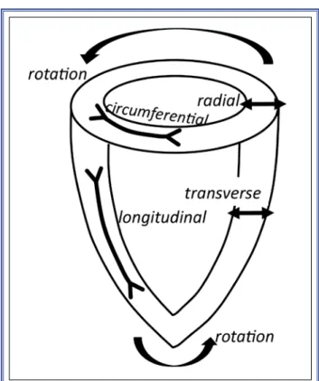
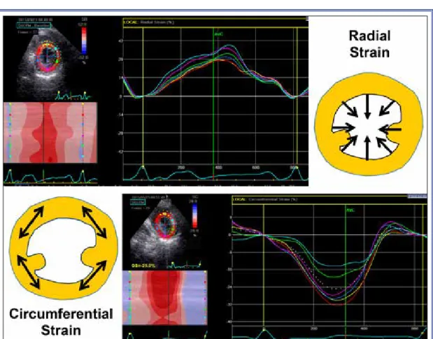
peckle tracking imaging (STI) has gained wide clinical use in recent years as a means of quanti-fying myocardial mechanics. This technique follows speckles seen on grayscale images that are the result of backscattered ultrasound from structures smaller than the ultrasound wavelength. Random noise is filtered out and temporally stable blocks of speckles are tracked from frame to frame in multiple regions within the image plane using a block matching algo-rithm (Figure 1). This provides the information of lo-cal displacement and geometric shift of the speckles relative to each other and provides strain data at first step, unlike tissue Doppler imaging, in which basal data is velocity. Naturally, this technique necessitates high quality 2-dimensional (2D) images. STI is not dependent on Doppler principle. With this technique, the entire left ventricular (LV) wall can be analyzed. The regions of interest (ROI) are not limited to any particular region or direction of deformation. Conse-quently, STI enables quantification of deformation in longitudinal, radial, and circumferential directions, as well as quantification of rotation (Figure 2).Strain indicates percent of deformation during the cardiac cycle. This percent of change is expressed in relation to a reference length, which is usually the end-diastole (closure of the mitral valve). The notation of strain values should always include a sign. As a re-sult, longitudinal LV strain is a negative deformation (Figure 3). The radial strain is represented by positive curves, indicating thickening in the short axis (SAX)
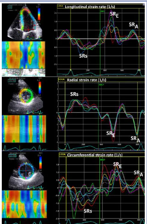
toward the cavity center, and the circumferential strain is represented by negative curves, indicating tangential shortening in the SAX plane (Figure 4). The correspond-ing strain rate (SR) data are also readily available. The
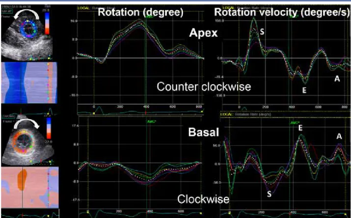
systolic SR with a positive sign for radial deformation and a negative sign for longitudinal and circumferential deformations, while the diastolic SR waves (ESR and ASR) have the opposite signs of systolic component, similar to the tissue velocity data (Figure 5). The apical and basal rotation can also be quantified from the dis-placement of speckles around the LV long axis. Figure 6 illustrates the rotation curves and the rotation velocities, and Figure 7 demonstrates the twist curve derived from the difference between the apical and basal rotations.
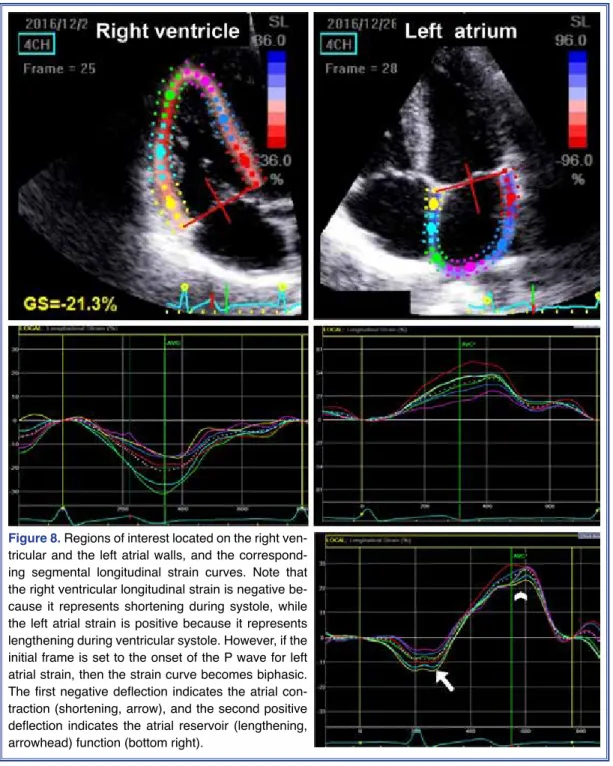
The right ventricular (RV) longitudinal strain and the atrial longitudinal strain can also be derived from properly aligned RV-focused and left atrial-focused apical images (Figure 8). Quantification of other strain components for these chambers are less well established due to their thin walls and relatively com-plicated anatomy of the RV.
Of note, the speckle tracking technique is applicable with almost all echocardiography devices, though some-times different names are used, such as velocity vector imaging (Figure 9). Also note that the transverse strain indicates percent wall thickening on the apical views, Received:January 20, 2017 Accepted:January 23, 2017
Correspondence: Dr. Leyla Elif Sade. Başkent Üniversitesi Tıp Fakültesi, Kardiyoloji Anabilim Dalı, Ankara, Turkey..
Tel: +90 312 - 212 90 65 e-mail: [email protected] © 2017 Turkish Society of Cardiology
Abbreviations:
AVC Aortic valve closure LV Left ventricle ROI Region of interest RV Right ventricle SAX Short-axis SR Strain rate
presumably equivalent to radial strain on the SAX. Advantages of STI are that this technique • is angle independent (almost),
• provides direct measurement of segmental de-formation,
• allows assessment of all segments, including the apex, and
• quantifies deformation occurring in more than 1 direction.
Image acquisition
Optimal image acquisition necessitates the following: • Good image quality. Artifacts, reverberations, and poorly visualized myocardium compro-mise tracking quality. Any artifact that resem-bles speckle patterns outside the myocardium will be tracked and compromise the validity of the data (Figure 10).
• Frame rate (optimization) between 40-80 fps. higher frame rate compromises tracking by re-ducing the spatial resolution. For short-lived mechanical events, such as isovolumic events, high frame rate is needed. Higher frame rate is particularly important for velocity and SR mea-surements, and also when the heart rate is high, such as during stress echocardiography. These situations may limit the use of STI in its current state.
• Coverage of complete heart cycle, paying at-tention to the reference frame, in order to avoid erroneous peak values.
• Apical foreshortening and oblique SAX images seriously affect the results.
Data processing
• ROI should be adjusted in order to:
- incorporate wall thickness in the analysis, while avoiding the pericardium and extracardiac spaces, and
Turk Kardiyol Dern Ars
198
Figure 1. The speckle tracking technique follows temporally stable blocks of speckles from frame to frame on grayscale images
Thus, local displacement and geometric shift of the speckles relative to each other provide an estimation of tissue deformation, which forms the base of strain data.
Figure 2. One-dimensional strain components that can be
Figure 3. The longitudinal strain curves from 6 segments of the apical 4-chamber view are presented in the panel at right. Curves are negative, representing the segmental shortening during systole. More negative values represent good function, less negative values represent impaired function. Increases in longitudinal strain indicate that the numbers are becoming more negative, while decreases in longitudinal strain mean that numbers are becoming less negative and that the left ventricular function is deteriorating. The lower left panel is the M-mode color-coded strain profile. Red hues indicate shortening, blue hues indicate lengthening. Note that the cardiac cycle is adjusted to the mitral valve closure.
Figure 4. The upper panel displays the radial segmental thickening, and the lower panel illustrates circumferential
- track the wall properly according to visual impres-sion.
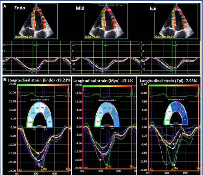
ROI should be divided into segments of equal distances. Sixteen- or 18-segment model is recom-mended. Inclusion of the pericardium will result in erroneously reduced values. Meanwhile, ROI is not restricted to the entire wall thickness or the
endocar-dium; endocardial, midwall, and epicardial layers can be assessed separately. Each of these contours can be defined manually or generated automatically. It is im-portant to clearly define which layer or segment is measured in order to avoid erroneous comparisons. Usually, no selection of layer will give the mid-myo-cardial result. Measurements obtained are highest in the endocardial layer and lowest in the epicardial
Turk Kardiyol Dern Ars
200
Figure 5. Longitudinal (upper panel), radial (middle panel), and circumferential (lower
layer in a healthy heart (Figure 11).
• Smoothing. Temporal and spatial smooth-ing level can be manually adjusted. Minimum necessary smoothing may be helpful to better distinguish the curve behavior, but excessive smoothing should always be avoided.
• Definition of end-diastole and the beginning of cardiac cycle (baseline reference length). Initial reference length between these 2 points is im-portant. Any deformation, i.e., strain, is calcu-lated in relation to the initial length as percent shortening or lengthening. Also, remember that it is imperative to cover the complete cardiac cycle. When the strain tracings appear to be nonphysiological, 1) suboptimal tracking and 2) cardiac cycle not adjusted to correct refer-ence frame should be considered first as poten-tial causes of error (Figures 9, 10).
• Similar (almost the same) cycle lengths should be recorded to obtain global strain estimation or twist (Figure 12a, b). Data from different cy-cle lengths cannot be combined. Global longi-tudinal strain and global circumferential strain permit combination of strain data from 3 dif-ferent image planes only if the curves are time-aligned. This limitation can be circumvented with the use of 3D data set if the patient has beat-to-beat variation, as in atrial fibrillation.
Figure 6. (Left) The counterclockwise rotation of the apex is represented by the positive curves and the clockwise rotation of
the base is represented by the negative curves. The rotation is measured in degrees. (Right) The velocity of rotation can also be quantitated. Dotted curves indicate the global rotation and rotation velocity of the corresponding cut plane.
Figure 7. Left ventricular twist is calculated as the net
differ-ence of rotation at isochronal time points between the apical and basal short-axis planes.
Visual display of data
Data presentation should be clearly defined in terms of
- Segments, layers that are presented.
- Deformation components, i.e., longitudinal, circumferential, radial and area strain. Values obtained are the estimation of strain in 1D. If a segment is shortening in the longitudinal plane, it will thicken in the radial or transverse
planes. Shortening in the circumferential plane will result in thickening in the radial plane and vice versa because of fiber rearrangement and cross-fiber shortening.
- Global longitudinal, global circumferential strain. Note that the global longitudinal or cir-cumferential strain is not equal to the average of segmental peaks; rather, these represent in-stantaneous averaging of segmental curves.
Turk Kardiyol Dern Ars
202
Figure 8. Regions of interest located on the right
ven-tricular and the left atrial walls, and the correspond-ing segmental longitudinal strain curves. Note that the right ventricular longitudinal strain is negative be-cause it represents shortening during systole, while the left atrial strain is positive because it represents lengthening during ventricular systole. However, if the initial frame is set to the onset of the P wave for left atrial strain, then the strain curve becomes biphasic. The first negative deflection indicates the atrial con-traction (shortening, arrow), and the second positive deflection indicates the atrial reservoir (lengthening, arrowhead) function (bottom right).
Interpretation of the strain curve Steps to follow:
- Define which component of the myocardial
de-formation is represented,
- Look at the behavior of the entire curve, - Define the aortic valve closure (AVC), and - Consider both amplitudes and timing of the peaks.
Figure 10. Automatically defined cardiac cycle that starts at non-QRS electrical activity, which
is usually an artifact, premature ventricular beat, or prominent P wave. As a result, strain curves are senseless.
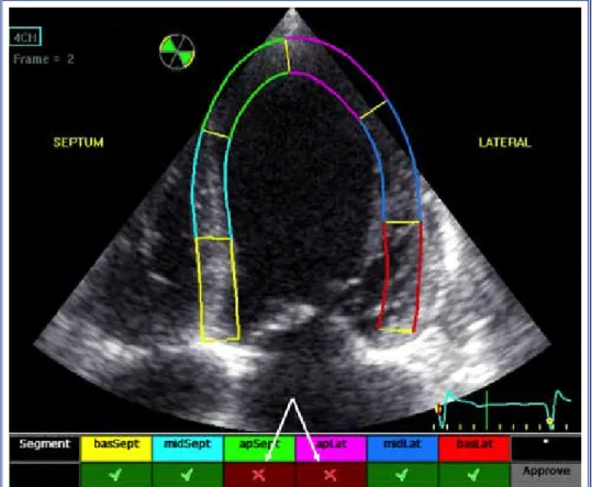
Figure 9. Example of poor quality image not suitable for tissue tracking: poorly delineated
endocardium, poor visualization of apical segments, and the region of interest beyond the myocardium. The software indicates poor tracking of apical segments (arrows).
Segment that is deforming after AVC will not con-tribute to ejection, whatever the amplitude may be. Therefore, it is important to define precisely which peak is measured: 1) any peak during the cardiac cycle, regardless of AVC, 2) peak systolic strain (the peak before AVC), 3) end-systolic strain (at AVC), or 4) post systolic strain (Figure 13).
Limitations
• Analyses require off-line processing and cannot be performed during live study.
• Frame rate is currently restricted to 40-90 fps, which is not suitable for high heart rates.
• Data set that is 2D allows 1D assessment of defor-mation. Feasibility and reproducibility are best for longitudinal strain using STI. Strain quantification
based on 3D data set is also feasible today; how-ever, the frame rate is even less than 2D speckle tracking. On the other hand, 3D data set provides area strain information, which is a combination of the longitudinal and circumferential strain.
• Intervendor differences in measurements have to be taken into account, particularly for serial as-sessment of the patients and when making com-parisons. The same machine and software should be used for serial follow-up and comparisons. • Through-plane motion of the speckle patterns on
2D images is unavoidable and is a source of error, mostly in the SAX plane.
Proposed readings
Voigt JU, Pedrizzetti G, Lysyansky P, Marwick TH,
Turk Kardiyol Dern Ars
204
Figure 11. Layer-specific strain analyses. Endocardial, mid-myocardial, and epicardial segmental longitudinal
strain curves from 2 different software examples (A, B). Note that values are decreasing from endocardium toward epicardium.
A
Houle H, Baumann R, et al. Definitions for a common standard for 2D speckle tracking echocardiography: consensus document of the EACVI/ASE/Industry Task Force to standardize deformation imaging. J Am Soc Echocardiogr 2015;28:183-93.
Mor-Avi V, Lang RM, Badano LP, Belohlavek M, Cardim NM, Derumeaux G, et al. Current and evolv-ing echocardiographic techniques for the quantitative evaluation of cardiac mechanics: ASE/EAE
conssus statement on methodology and indications en-dorsed by the Japanese Society of Echocardiography. Eur J Echocardiogr 2011;12:167-205.
Farsalinos KE, Daraban AM, Ünlü S, Thomas JD, Badano LP, Voigt JU. Head-to head comparison of global longitudinal strain measurements among nine different vendors: The EACVI/EASE Inter-vendor comparison study. J Am Soc Echocardiogr 2015;28:1171-81.
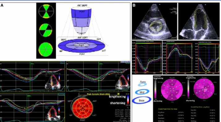
Figure 12. (A) Display of global longitudinal strain. Left ventricular cut planes from apical 4-chamber, 2-chamber, and apical long
axis views with similar cycle length are combined in the bull’s eye format. (B) Upper panel illustrates velocity vector imaging (an-other vendor) with superimposed arrows indicating endocardium that show velocity vectors in the parasternal short axis and apical 4-chamber views. Middle panel represents segmental circumferential, radial, and longitudinal strain curves. Lower panel is the bull’s eye display of global circumferential and longitudinal strain. Note that this vendor provides global circumferential strain data in addition to global longitudinal strain. However this latter vendor’s global value only represents the average of the segmental peaks instead of the peak of the average curve of all the segments.
Figure 13. (A) Normal longitudinal strain curve, (B) longitudinal strain with reduced systolic strain but increased post systolic
strain, suggesting a pathological situation, such as ischemia or pressure overload, (C) normal septal strain but late lateral strain not contributing to ejection, despite the preserved peak strain value.