Determination of periodically collapsing rational bubbles

DETERMINATION OF PERIODICALLY COLLAPSING RATIONAL BUBBLES A Master’s Thesis by SAVAŞ KUŞ The Department of Economics Bilkent University Ankara September 2006

DETERMINATION OF PERIODICALLY COLLAPSING RATIONAL BUBBLES

The Institute of Economics and Social Sciences of

Bilkent University

by

SAVAŞ KUŞ

In Partial Fulfillment of the Requirements for the Degree of MASTER OF ARTS

in

THE DEPARTMENT OF ECONOMICS BILKENT UNIVERSITY

ANKARA

I certify that I have read this thesis and have found that it is fully adequate, in scope and in quality, as a thesis for the degree of Master of Arts in Economics.

--- Asst. Prof. Taner Yiğit Supervisor

I certify that I have read this thesis and have found that it is fully adequate, in scope and in quality, as a thesis for the degree of Master of Arts in Economics.

--- Asst. Prof. Refet Gürkaynak Examining Committee Member

I certify that I have read this thesis and have found that it is fully adequate, in scope and in quality, as a thesis for the degree of Master of Arts in Economics.

--- Asst. Prof. Levent Akdeniz Examining Committee Member

Approval of the Institute of Economics and Social Sciences

--- Prof. Erdal Erel

ABSTRACT

DETERMINATION OF PERIODICALLY COLLAPSING RATIONAL BUBBLES

Kuş, Savaş

M.A., Department of Economics Supervisor: Asst. Prof. Taner Yiğit

September 2006

Since Evans’ criticism of conventional unit root and cointegration tests in case of periodically collapsing rational bubbles, a number of new approaches have been suggested. In this paper, we propose a new testing strategy to overcome the detection problem of periodically collapsing rational bubbles. Our method is based on Threshold Autoregressive Stochastic Unit Root Models. Monte Carlo simulations show that the proposed testing strategy is successful at the detection of bubbles introduced in Evans (1991). Besides having detection power, we are able to estimate threshold level and probability of collapse of bubbles. The empirical findings for US stock price in the 1871-2004 period are in favor of existence of bubbles.

ÖZET

PERİYODİK OLARAK ÇÖKEN RASYONEL BALONLARIN BELİRLENMESİ

Kuş, Savaş

Yüksek Lisans, Ekonomi Bölümü Tez Yöneticisi: Yr. Doç. Dr. Taner Yiğit

Eylül 2006

Evans’ın, periyodik olarak çöken rasyonel balonlar söz konusu olduğunda geleneksel birim kök ve eşgüdümlü birim kök testlerine getirdiği eleştiriden sonra yeni bir çok yaklaşım öne sürülmüştür. Bu çalışmada, periyodik olarak çöken rasyonel balonların belirlenebilmesi sorununun üstesinden gelmek için yeni bir metod önerilmektedir. Metodumuz Eşik Ardışık Bağımlı Rastlantısal Birim Kök Modelleri’ne dayanmaktadır. Monte Carlo simülasyonları önerilen testin Evans (1991) çalışmasında sunulan tipten balonların belirlenebilmesi konusunda başarılı olduğunu göstermektedir. Balonların belirlenebilmesi konusunda etkili olmamızın yanında, eşik düzeyini ve balonların çökme olasılıklarını tahmin edebilmekteyiz. 1871-2004 yılları arasında ABD hisse senedi fiyatları için elde edilen ampirik bulgular balonların varlığını destekleyici yöndedir.

TABLE OF CONTENTS

ABSTRACT ... iii

ÖZET ... iv

TABLE OF CONTENTS ... v

LIST OF TABLES ... vi

LIST OF FIGURES ... vii

CHAPTER 1: INTRODUCTION ... 1

CHAPTER 2: LITERATURE REVIEW ... 5

2.1 Standard Model for Stock Prices... 5

2.2 Integration/Cointegration Based Tests... 8

2.3 Evans’ Criticism... 15

2.4 Detection of Periodically Collapsing Rational Bubbles... 19

CHAPTER 3: METHODOLOGY ... 27

3.1 Threshold Autoregressive Stochastic Unit Root Models... 27

3.2 Utilizing TARSUR to Detect Periodically Collapsing Rational Bubbles...30

CHAPTER 4: SIMULATIONS AND RESULTS... 33

4.1 Monte Carlo Simulations... 33

4.2 Simulation Results... 38 4.3 Empirical Results... 42 CHAPTER 5: CONCLUSION ... 45 SELECT BIBLIOGRAPHY ... 47 APPENDICES ... 50 APPENDIX A ... 50 APPENDIX B ... 52 APPENDIX C ... 53 APPENDIX D... 54

LIST OF TABLES

Table 1: Sample Autocorrelations for Real Stock Prices, Dividends and Their First

Differences...10

Table 2: Dickey-Fuller Test Results (No Lags)...11

Table 3: Dickey-Fuller Test Results (Four Lags) ... 11

Table 4: Bhargava Tests of the Random-Walk Hypothesis ... 13

Table 5: Bhargava Tests for Simulated Bubbles... 16

Table 6: Unit Root Test Results for Simulated Stock Prices with Bubbles... 17

Table 7: Cointegration Test Results for Simulated Stock Prices with Bubbles... 18

Table 8: Test Results for Typical Simulation... 18

Table 9: Percentage rejections of Markov Switching ADF tests…... 21

Table 10: Performances of van Norden and Hall&Sola Tests ... 22

Table 11: Percentage of Rejections of Non-cointegration Between Price and Dividend Series (Taylor and Peel, 1998)... 23

Table 12: Percentage of Correct Rejections of the Null Hypothesis (Bohl, 2003) ... 26

Table 13: Scale Factors Used for Different Probability of Collapses ... 35

Table 14: Percentage of Correct Rejections of the Null Hypothesis ...38

Table 15: Simulation Results ... 40

LIST OF FIGURES

Figure 1: Simulated Price Series... 54 Figure 2: Simulated Bubble Series... 54 Figure 3: Monthly US Stock Prices and Residuals...55

CHAPTER 1

INTRODUCTION

The problem of the detection of asset price bubbles has attracted many researchers in the past twenty years. Detection of asset price bubbles has crucial importance not only academically, but also economically and financially. One can especially think of a very striking example to evaluate the importance of the detection of asset price bubbles, namely the 1990s recession in Japan. Lots of economists believe that the collapse of asset price bubbles pushed Japan in such a big recession that their recovery to this day is incomplete. Another example given as the effect of bubbles is stock market crash in Asian markets that took place in 1997. Although it is difficult to demonstrate that what put Japan or other Asian countries in such a situation was a collapse of asset price bubbles, detection of bubbles is still a very important topic to be investigated. In this study we deal with the problem of detecting periodically collapsing rational bubbles. If there exist, periodically collapsing and reoccurring nature of most asset price bubbles in real life and the difficulty in detecting them make Evans’s class of bubbles set a very important and challenging topic to study.

Since the measurement of the fundamental price of an asset is quite difficult, more than several papers have so far taken on the arduous task of identifying

whether financial markets could have bubbles from time to time even in the existence of complete rationality. Among the methods suggested for testing rational bubbles, one can start with variance bounds tests of Schiller (1981) and LeRoy and Porter (1981). Next is West employing two step tests (1987, 1988) to detect rational bubbles. Another methodology later developed relies on (co)integration based tests (Diba and Grossman, 1988b). By applying these tests, Diba and Grossman (1988b) show that there are no bubbles in US stock prices. However, Evans (1991) shows that (co)integration based tests fail for an important class of rational bubbles, the ones that collapse periodically. Evans shows that these bubbles appear to be stationary when standard unit root tests are applied. Utilizing Monte Carlo simulations, he also shows the poor performance of (co)integration based tests. In response to Evans’ criticism, a number of new approaches have been suggested to overcome the detection of periodically collapsing bubbles. Among them are Hall et al. (1999), van Norden (1996), Taylor and Peel (1998), Wu and Xiao (2002), Scacciavillani (1994) and Bohl (2003).

We take Threshold Autoregressive Stochastic Unit Root (TARSUR) test of Gonzalo and Montesinos (2002) as basis. We modify these tests by altering the assumption that the expected autoregressive coefficient is equal to one. The main idea of the test is based on the determination of two different regimes where one of which is mildly nonstationary and the other one is explosive. In contrast to the conventional unit root based tests, our proposed approach has its advantage in dealing with collapsing bubbles. Applying simulation studies, we show that the proposed testing strategy is successful in the detection of bubbles introduced in Evans (1991). Our test is superior to most of the other approaches suggested to

overcome the detection of periodically collapsing bubbles for high probabilities of collapses. Although some of the earlier studies are more successful for low probabilities of collapses, due to high power of (co)integration tests we make up for it with significantly higher success where earlier tests fail.

Although our test is powerful compared to other tests, what makes our study distinct is that we are able to estimate the threshold level and probability of collapse of a bubble when and if it exists. None of the studies, suggested for detecting problem of periodically collapsing rational bubbles, have tried to estimate these critical features of bubbles. Aside from being the first in estimation of these values, simulations in our study show that we are quite successful at obtaining the threshold level and probability of collapses. Estimating probability of collapse and threshold levels makes one to analyze a moderate chunk of the finance literature, namely trend chasing, where investors don’t want to be left out of the increasing market even though they know that the market is in a bubble.

We do not only carry out the test with artificial data, but also investigate if there are periodically collapsing rational bubbles in real US stock price series. Early studies generally conclude in favor of nonexistence of bubbles except Hall and Sola (1993). Among the ones who find evidence of nonexistence of bubbles are van Norden (1996), Taylor and Peel (1998), Wu and Xiao (2002) and Bohl (2003). Using both monthly and annual stock price and dividend data from Standard and Poor’s 500 stock price and dividend series from 1871 to 2004, we find evidence in favor of the existence of bubbles.

The plan of the paper is as follows: Chapter 2 gives a review of existing literature on the detection of periodically collapsing rational bubbles. Chapter 3 describes the suggested methodology. Chapter 4 discusses simulation and empirical results, and Chapter 5 concludes.

CHAPTER 2

LITERATURE REVIEW

In this chapter, we will first give a brief background on standard model for stock prices and conventional tests for the detection of asset price bubbles. Then, with the introduction of periodically collapsing rational bubbles, Evan’s criticism to conventional tests will be presented. Finally, different approaches to overcome detection problem of such bubbles will be discussed.

2.1 Standard Model for Stock Prices

Utilizing standard assumptions of no arbitrage and rational expectations, consumers’ utility maximization problem can be applied to determine basic asset pricing relationship. The maximization problem is as given:

Max ⎭ ⎬ ⎫ ⎩ ⎨ ⎧

_∑

where p is the price of the asset, _t d is the dividend paid for the asset, _t e_t+i is the endowment, a_t+i is the storable asset, u(c_t)is the utility driven from the consumption c , and _t β is the constant discount rate. E denotes expectations _t conditional on information at date t.

The first order condition of the optimization problem is the following:

E_t

{

}

{

[

]

}

Standard model for stock prices assumes a linear utility function. Moreover, assuming the existence of a riskless bond available in zero net supply with an interest rate r, equation (1) becomes:

( ). 1 1 ) ( _{t i1 t t i t i} t E p d r p E _{+− +} + ₊ + = (2)

The solution can be reached by iterating this first degree difference equation further: p_t =F_t +B_t. (3) such that E_t(B_t+1)=(1+r)B_t. (4) where

∑

Equation (5) defines the forward looking solution to (2), while (3) gives the general solution which is the sum of a market fundamental component F , and a _t bubble component B whose existence does not conflict with the rational _t expectations assumption. Notice that existence of a rational bubble is not in conflict with no arbitrage assumption, equation (4) ensures the validity of no arbitrage.

From (4), the following relation can be reached:

j _t j

t

t B r B

E ( ₊ )=(1+ ) (6)

Equation (6) says that if B is nonzero, then the expected value of rational _t bubbles component,E_t(B_t+j), increases or decreases at the geometric rate (1+ r); and since r >0, ₊ =±∞

∞

→ ( )

lim _{t t j}

j E p depending on the sign of the B (Diba and t Grossman 1998a).

Assume that B is negative, then for some j, _t E_t(p_t+j) becomes negative which means that stockholders rationally expect negative prices. However, such a situation is not possible given free disposal. Therefore, B cannot be negative. As _t shown in (Diba and Grossman 1998a), it cannot be positive also. The solution to equation (4) is:

B_t+1 −(1+r)B_t =z_t+1, (7)

where z is a random variable with _t+1 E_t(z_t+i)=0 for all i>0.

If B is zero, the bubble will start with the next nonzero realization of _t z . If _t+1

1 +

t

z is negative, B will be negative, too. Then as mentioned above, this causes the _t+1 stock price to be negative in finite time. Thus, z cannot be negative. Now, assume _t+1 that it is positive, then next realizations must also be negative to ensure E_t(z_t+i)=0 which is the no arbitrage assumption. However, as it is shown, z cannot be _t+1 negative, so if B is zero, then _t z equals zero with probability one. This means _t+1 that if there is no bubble at time t, then it cannot start in future. In other words, if there exists a bubble today, it must have started from the first day of trading of the stock.

2.2 Integration/Cointegration Based Tests

Diba and Grossman do not only bring up theoretical arguments to show nonexistence of bubbles, but also develop empirical tests for the detection of explosive rational bubbles allowing for unobservable variables and different valuations of future dividends and capital gains (Diba and Grossman 1998b).

The stock price is equal to present value of next period’s expected price, dividend and an unobservable variable:

( ), 1 1 1 1 1 + + + + + + = _{t t t t} t E p d u r p α (8)

where α is a positive constant valuating future dividends relative to future capital gains, and u is the unobservable variable._t 1 Market fundamental component of the stock price is:

∑

As before, the general solution to equation (8) is:

t t t F B p = +

where E_t(B_t+1)=(1+r)B_t

Assume that u is not more nonstationary than _t d . Then, if there is no _t bubble, stock prices should be as stationary as market fundamental. For example, if dividends and unobservable variables are nonstationary in levels, but stationary in first differences, then stock prices is also stationary in first differences in the absence of bubbles. However, if stock prices contain a rational bubble, then the nth difference of bubble will be:

[

]

where z is a random variable with _t E_t(z_t+i)=0 for all i>0 as given in equation (7).

1 _{Since allowing for different valuations of expected dividends and capital gains does not alter central}

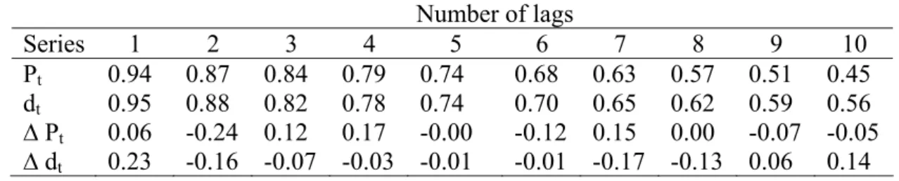
Diba and Grossman (1998b) reveal that for simple specifications of z , such _t as white noise, regardless of how many times differenced, the bubble process will be nonstationary. Thus, asset price will be nonstationary, too. They exploit this fact to test for the presence of rational bubbles in stock prices using Standard & Poor’s Composite Stock Price Index and dividend series for this portfolio of stocks from 1871 to 1986. They firstly find sample autocorrelations for these real stock prices and dividends, and their first differences:

Table 1. Sample Autocorrelations for Real Stock Prices, Dividends and Their First Differences Number of lags Series 1 2 3 4 5 6 7 8 9 10 Pt 0.94 0.87 0.84 0.79 0.74 0.68 0.63 0.57 0.51 0.45 dt 0.95 0.88 0.82 0.78 0.74 0.70 0.65 0.62 0.59 0.56 ∆ Pt 0.06 -0.24 0.12 0.17 -0.00 -0.12 0.15 0.00 -0.07 -0.05 ∆ dt 0.23 -0.16 -0.07 -0.03 -0.01 -0.01 -0.17 -0.13 0.06 0.14

Diba and Grosman (1998b) suggest nonstationary means for original price and dividend series by looking at the path of autocorrelation, whereas their first differences show clues of mean stationarity supporting nonexistence of bubbles.

They do not only consider autocorrelation patterns, but apply Dickey-Fuller unit root tests to see if there is something unexplained by the standard model for stock prices which can be attributable to the existence of rational bubbles. They estimate the following model:

k _t i i t i t t t x x x =µ+γ +ρ +

∑

The results of the estimation can be shown in Tables 2 and 3.

Table 2. Dickey-Fuller Test Results (No Lags)

Series: Pt dt ∆ Pt ∆ dt µˆ 0.0058 (0.0166) (0.0005) 0.0007 (0.0168) 0.0002 (0.0004) 0.0001 γˆ 0.0006 (0.0003) 0.00003 (0.00001) 0.0001 (0.0003) 0.000001 (0.000006) ρˆ 0.90 (0.04) 0.87 (0.05) 0.06 (0.10) 0.23 (0.10) Standard error of estimate 0.071 0.002 0.072 0.002 3 Φ 2.55 3.43 42.38 30.89

Note: Table presents the results of the model in equation (11) with k=0. Standard errors of

coefficients are in parentheses. Φ₃ is the F-statistic which test the null hypothesis (γ,ρ)=(0,1).

Critical value for Φ₃ is 5.47 and 6.43 for 10 % and 5 % significance levels respectively.

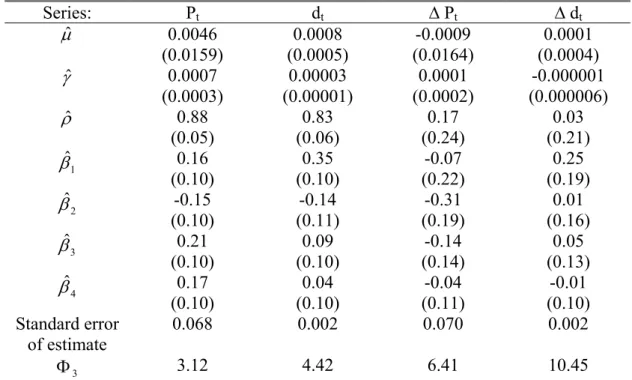
Table 3. Dickey-Fuller Test Results (Four Lags)

Series: Pt dt ∆ Pt ∆ dt µˆ 0.0046 (0.0159) 0.0008 (0.0005) -0.0009 (0.0164) 0.0001 (0.0004) γˆ 0.0007 (0.0003) 0.00003 (0.00001) 0.0001 (0.0002) -0.000001 (0.000006) ρˆ 0.88 (0.05) 0.83 (0.06) 0.17 (0.24) 0.03 (0.21) 1 ˆ β 0.16 (0.10) 0.35 (0.10) -0.07 (0.22) 0.25 (0.19) 2 ˆ β -0.15 (0.10) (0.11) -0.14 (0.19) -0.31 (0.16) 0.01 3 ˆ β 0.21 (0.10) 0.09 (0.10) -0.14 (0.14) 0.05 (0.13) 4 ˆ β 0.17 (0.10) 0.04 (0.10) -0.04 (0.11) -0.01 (0.10) Standard error of estimate 0.068 0.002 0.070 0.002 3 Φ 3.12 4.42 6.41 10.45

Note: Table presents the results of the model in equation (11) with k=4. Standard errors of

coefficients are in parentheses. Φ₃ is the F-statistic which test the null hypothesis (γ,ρ)=(0,1).

The results in Tables 2 and 3 indicate that both real price and dividend series are nonstationary in levels, but stationary in first differences. Thus Diba and Grossman conclude that there are no bubbles. Besides using Dickey-Fuller test, they also offer another method to test for the existence of bubbles based on cointegration.

To give the idea behind using cointegration tests, we rearrange equation (9)2:

∑

∑

Putting (12) into (3), we obtain:

( .) 1 1 ) ( 1 1 1 1 1 1 1

∑

∑

Diba and Grossman argue that if u is stationary in levels and _t d is _t stationary in first differences, in the absence of bubbles the right hand side of equation (13) is stationary which means although price and dividend series are nonstationary, linear combination of them is stationary, e.g. price and dividend series are cointegrated of order (1,1) with cointegration vector (1,-r-1). In other words, under the null hypothesis of no bubbles, price and dividend series should be cointegrated. They use this fact to test for the presence of bubbles.

Firstly, they use cointegration tests developed by Granger and Engle (1987). One test uses the Durbin-Watson statistic of the cointegrating regression. Other tests employ Dickey-Fuller regressions:

∑

Diba and Grossman calculate ξ2 and ξ3 statistics which correspond to t-ratios

for ρ with k equal to zero and four respectively.

Cointegration test based on Durbin-Watson statistic of cointegrating regression results in rejection of the null hypothesis of no cointegration at 1 percent critical level. However, ξ2 statistic rejects the null at 5 percent, while ξ3 fails to

reject even at 10 percent. Due to the inconsistency of results of different testing approaches, the authors use Bhargava ratios which are claimed to yield the most powerful tests of random-walk hypotheses against stationary and explosive alternatives. The results of Bhargava tests can be seen in Table 4.

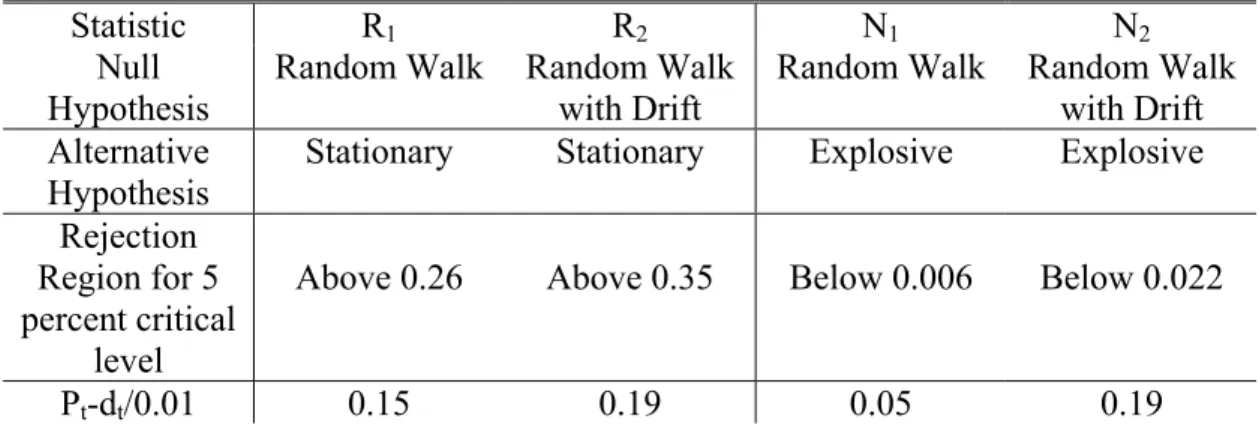
Table 4. Bhargava Tests of the Random-Walk Hypothesis

Statistic R1 R2 N1 N2

Null

Hypothesis Random Walk Random Walk with Drift Random Walk Random Walk with Drift Alternative

Hypothesis

Stationary Stationary Explosive Explosive Rejection Region for 5 percent critical level Above 0.26 Above 0.35 Below 0.006 Below 0.022 Pt-dt/0.01 0.15 0.19 0.05 0.19

Table 4 (cont’d) Pt-dt/0.02 0.40 0.45 0.12 0.64 Pt-dt/0.03 0.62 0.60 0.31 1.11 Pt-dt/0.04 0.48 0.49 0.44 0.97 Pt-dt/0.05 0.35 0.38 0.35 0.76 Pt-dt/0.06 0.28 0.32 0.26 0.62 Pt-dt/0.07 0.24 0.27 0.21 0.53 Pt-dt/0.08 0.21 0.25 0.18 0.47

As it is seen from Table 4, R1 and R2 statistics rejects the null hypothesis of

random walk for r between 0.02 and 0.06, and random walk with drift for r between 0.02 and 0.05 respectively. However, N1 and N2 statistics which test for random

walk and random walk with drift against one-sided explosive alternative cannot reject the null hypothesis of unit root. Hence, using Bhargava tests, Diba and Grossman find strong evidence of cointegration between price and dividend series, and conclude that there is no bubble in stock prices.

After using cointegration tests to test for bubbles, Diba and Grossman (1998b) apply their tests to artificial data to confirm that their approaches can detect bubbles. They take r equal to 0.05 and generate a bubble series using equation (7) with standard normal innovations. Both N1 and N2 statistics reject the null

hypothesis of unit root against explosive alternatives at 5 percent level in 95 of 100 simulations.

As mentioned in Diba and Grossman (1998b), there is a critical point about the explanation of the results of unit root and cointegration tests which needs to be clarified. It may not be true to conclude in favor of presence of bubbles after applying these tests and finding that prices are more nonstationary than dividends or

price and dividend series are unit root but not cointegrated, because these results may stem from the inappropriateness of the assumption made about unobserved fundamentals. However, Diba and Grossman discuss that although a finding that cannot reject the presence of bubbles may not prove that there is bubble, rejection of bubble hypothesis is a proof of absence of bubbles. Yet, as Evans shows, this conclusion is also problematic.

2.3 Evans’ Criticism

Evans (1991) shows that unit root and cointegration based tests suggested by Diba and Grossman (1998b) fail for an important class of rational bubbles, which collapse periodically. He generates artificial bubbles which are explosive and apply integration/cointegration tests to price series including artificial bubbles. Simulations show that stock prices do not appear to be more nonstationary than dividends when prices contain explosive bubbles with considerable size and volatility.

Evans (1991) examines the following class of rational bubbles:

⎪ ⎩ ⎪ ⎨ ⎧ > ⎥ ⎦ ⎤ ⎢ ⎣ ⎡ ⎟ ⎠ ⎞ ⎜ ⎝ ⎛ + − + + ≤ + = + + + + δ _{θ α} π δ α t t t t t t t t _{u if B} r B r B if u B r B 1 1 1 1 1 ) 1 ( ) 1 ( (15)

where δ and α are positive parameters such that 0<δ <(1+r)α, u_t+1 is i.i.d. positive random variable with E_t(u_t+1)=1 and θ_t+1 is an exogenous i.i.d. random Bernoulli process which takes the value 1 with probability π and 0 with probability (1-π) where 0<π≤1. Hence, the bubble increases at a mean rate (1+r) for small values of Bt, but after exceeding a threshold value α, it grows faster, with the

possibility of collapsing with probability (1-π). When it collapses, the process begins again with a mean value of δ .3

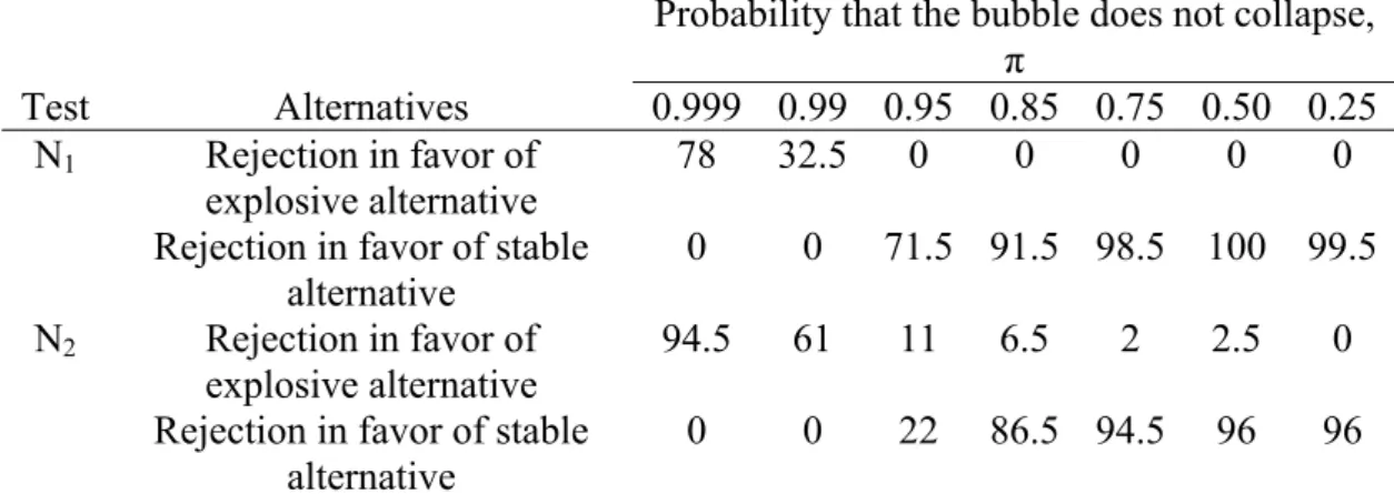
Evans firstly applies Bhargava tests used in Diba and Grossman (1998b) to artificially generated bubble series. For this, two hundred bubble series each having a sample size 100 are constructed according to equation (15) with r=0.05, α=1, δ =0.05, B1=δ and u_t =exp(y_t −τ2/2) where y_t ~IIN(0,τ2), τ=0.05. The results

of Bhargava tests are given in Table 5:

Table 5. Bhargava Tests for Simulated Bubbles

Probability that the bubble does not collapse, π

Test Alternatives 0.999 0.99 0.95 0.85 0.75 0.50 0.25 N1 Rejection in favor of

explosive alternative 78 32.5 0 0 0 0 0

Rejection in favor of stable alternative

0 0 71.5 91.5 98.5 100 99.5 N2 Rejection in favor of

explosive alternative 94.5 61 11 6.5 2 2.5 0

Rejection in favor of stable alternative

0 0 22 86.5 94.5 96 96

Note: Numbers in the table show the percentage of tests rejecting unit root at 5 percent level against

stable and explosive alternatives. 5 percent critical points are 0.006 and 0.17 for N1 for stable and

explosive alternatives, respectively; 0.022 and 0.26 for N2 for stable and explosive alternatives,

respectively.

3 _{As can be verified easily, bubble process does not let arbitrage opportunities to appear, because it}

It can be revealed from Table 5 that as the probability of collapse increases, the results of Bhargava tests deteriorate. For π close to unity, the results are not so bad, but when π≤ 0.95, the number of rejections in favor of stable alternatives is more than in favor of explosive ones. As π gets lower, the results get much worse. Evans explains that since the maintained hypothesis for the Bhargava tests is a first order linear autoregressive process, when a complex nonlinear process is applied, Bhargava tests do not lead correct results.

After using Bhargava tests, since bubbles are not directly observable, Evans examine tests based on observable stock price and dividend data. He generates artificial dividend and bubble series which are used to form price series, and then apply unit root and cointegration tests suggested in Diba and Grossman (1998b).4 The results of the tests are in Tables 6 and 7:

Table 6. Unit Root Test Results for Simulated Stock Prices with Bubbles Percentage of Dickey-Fuller Φ3 tests significant at the 5 percent level

Series

Number of lags P ∆P d ∆d

None 25 98.5 2.5 100 Four 7 93.5 4 90

Note: Dividends are generated as random walk with drift. Bubbles are constructed using equation (15) with π=0.85. Price series is equal to the sum of bubble and dividend series generated. There are

200 simulations with sample size equal to 100 for each simulation. Regressions are of the form xt = µ

+ γt + ρxt-1 + ∑βi∆xt-I + εt. Φ3 is the F-statistic which test the null hypothesis (γ,ρ)=(0,1).

Critical value for Φ₃ is 5.47 and 6.43 for 10 % and 5 % significance levels respectively.

4 _{Evans scale up bubble series by 20 to ensure that sample variance of first difference of bubble is}

Table 7. Cointegration Test Results for Simulated Stock Prices with Bubbles Percentage of cointegration tests significant at the 5 percent level

Test

ξ1=DW ξ2 ξ3

90 84.5 60

Note: Dividends are generated as random walk with drift. Bubbles are constructed using equation (15) with π=0.85. Price series is equal to the sum of bubble and dividend series generated. There are

200 simulations with sample size equal to 100 for each simulation. ξ1, ξ2 and ξ3 are CRDW, DF and

ADF tests which are described in Granger and Engle (1987). Cointegration tests are based on a regression of price on dividend and a constant.

Looking at Table 6, it can be verified that unit root tests are not successful in detection of bubbles in stock prices, because the detection of bubble means that price series are more nonstationary than dividend series which are not deducible from Table 6.

The results of cointegration test are not different than unit root tests. At least 60 percent of the cases, cointegration tests incorrectly conclude in favor of no bubbles.

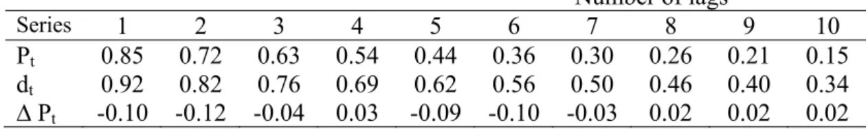
Finally, Evans report results of unit root and cointegration tests for a typical simulation. He generates 200 bubble and dividend series, chooses medians of these series, and construct price series using them. Then, he applies the same tests as in Diba and Grossman (1998b).

Table 8. Test Results for Typical Simulation A. Sample Autocorrelations: Number of lags Series 1 2 3 4 5 6 7 8 9 10 Pt 0.85 0.72 0.63 0.54 0.44 0.36 0.30 0.26 0.21 0.15 dt 0.92 0.82 0.76 0.69 0.62 0.56 0.50 0.46 0.40 0.34 ∆ Pt -0.10 -0.12 -0.04 0.03 -0.09 -0.10 -0.03 0.02 0.02 0.02

Table 8 (cont’d) ∆ dt -0.01 -0.17 0.01 -0.04 -0.06 -0.09 -0.03 -0.03 -0.02 -0.08 B. Dickey-Fuller Φ3 statistics: Series Number of lags Pt dt ∆ Pt ∆ dt None 5.13 4.19 58.56** _48.54** Four 4.68 4.15 13.42** 13.37** C. Cointegration tests: Test ξ1=DW ξ2 ξ3 0.561** -3.97* -3.51*

Note: (**) and (*) stands for 1 percent and 5 percent level significance, respectively.

Table 8 clearly indicates that there is no bubble in simulated stock price series. Unit root tests suggest nonstationarity for price and dividend series in levels but stationarity in first differences. Moreover, cointegration tests reject the null hypothesis of no cointegration between price and dividend. Hence both unit root and cointegration tests do not find bubble in stock prices.

In sum, Evans (1991) shows that standard unit root and cointegration tests are not successful in detection of periodically collapsing rational bubbles. After Evans’ criticism, some new approaches have been suggested to overcome the detection of periodically collapsing bubbles.

2.4 Detection of Periodically Collapsing Rational Bubbles

Hall et al. (1999) employ Markov switching Augmented Dickey-Fuller (ADF) unit root tests which allow for two separate regimes. Using this approach, they allow autoregressive parameter to change between two regimes in Evans’

periodically collapsing bubble equation (15). The suggested model is a different version of original ADF regression given in equation (11):

[

]

[

]

∑

where et is a sequence of i.i.d. random variable with zero mean and unit variance,

and s_t∈

{ }

q s s q s s p s s p s s t t t t t t t t − = = = = = = − = = = = = = − − − − 1 ) 0 | 1 Pr( ) 0 | 0 Pr( 1 ) 1 | 0 Pr( ) 1 | 1 Pr( 1 1 1 1 (17)

The authors test the null hypothesis of a unit root in either regime by using a recursive, non-linear filtering algorithm similar to that suggested in Hamilton (1994, pp. 692-694). It is stated that the existence of bubbles is consistent with φ₀>0 or

1

φ >0, because being φ₀ or φ bigger than zero indicates explosiveness of one of the ₁ regime. On the other hand, if φ₀ =φ₁ =0, then it can be said that there is no periodically collapsing rational bubble in stock prices.

Hall et al. (1999) apply Monte Carlo simulations to examine the capability of their testing strategy in detection of bubbles. They take the same parameters in Evans (1991) to generate artificial dividend and bubble series, and carry out bootstrapping techniques to get critical values. The results are in the following table:

Table 9. Percentage rejections of Markov Switching ADF tests t-tests 0 0 = φ vs. φ₀ <0 φ₁ =0 vs. φ₁ >0 DGP1 32.8 76.8 DGP2 33.2 74.2

Note: DGP1 and DGP2 use the same method and parameters given in Evans (1991). Bubble process

is given in equation (15) with π=0.85. The null hypotheses are φ₀ =0 and φ₁ =0

As it is seen from Table 9, the null hypothesis of φ₀ =0 cannot be rejected for 67.2 (66.8) percent for DGP1 (DGP2).5 However for the null hypothesis of

0 1 =

φ , the test rejects for 76.8 (74.2) percent for DGP1 (DGP2). In other words, for both of the Data Generating Processes, the tests correctly indicate that there are two regimes, one explosive and one nonstationary in more than 65 percent of the cases. However, the results are only for π=0.85. The performance of the test is not measured for other probabilities of collapse. Moreover, the authors do not apply their test to real stock price data.

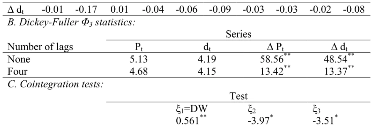
In another study, Van Norden and Vigfusson (1998) compare the performance of bubble tests suggested in van Norden (1996) and Hall and Sola (1993) which utilize Markov-switching ADF test which is explained before. Van Norden (1996) also uses switching regression system with switching probabilities as function of the relative size of the bubble. Van Norden and Vigfusson (1998) give the comparison results of the two methods as follows:

5 _{As it is seen from Table 9, the test rejects the null 0}

0 =

φ for 32.8 percent. In other words, it

cannot reject the null for 67.2 percent for DGP1 which means the first regime is nonstationary for 67.2 percent. Similarly, the null cannot be rejected for 66.8 percent for DGP2.

Table 10. Performances of van Norden and Hall&Sola Tests π

Test 0.999 0.99 0.95 0.85 0.75 0.50 0.25

van Norden % of rejections 1 5 16 48.5 77 28.5 3

Hall & Sola % of rejections 25 50 64 64 58 35

Note: The test suggested in Hall and Sola (1993) has not been done for π=0.999. Results are based on 5000 simulations. For both of the tests, the null hypotheses are the nonexistence of bubbles.

When compared to unit root and cointegration tests’ results, both of the tests are more successful, but as it is seen from Table 10, Hall and Sola (1993) test gives better results except π=0.75.

Van Norden and Vigfusson (1998) do not only carry out the tests with artificial data, but they also investigate if there is periodically collapsing rational bubbles in real stock price series. Using monthly S&P500 Index from January 1956 to July 1997, while Hall and Sola test finds strong evidence of bubbles, van Norden test does not reject the null hypothesis of no bubble.

Taylor and Peel (1998) propose a cointegration test which is robust to skewness and curtosis. Their method is based on a modification of Im (1996). They name their cointegration test statistic as residuals-augmented least squares (RALS) Dickey-Fuller statistic, CRτA. The results of their test are as follows:

Table 11. Percentage of Rejections of Non-cointegration Between Price and Dividend Series (Taylor and Peel, 1998)

π

0.99 0.95 0.85 0.75 0.50 0.25 CRτA % of rejections 0.00 0.00 0.00 0.00 48.90 51.64

Note: Results are based on 10000 simulations. Critical value for CRτA at 5 percent level is -3.790.

The null hypothesis is the non-cointegration of price and dividend series, meaning there is bubble.

Although the results of the test proposed in Taylor and Peel (1998) seem quite successful at a first glance, there are some important aspects behind data generating process used in Monte Carlo studies. The authors do not use the same parameters as in Evans (1991). They use their own estimations for parameters used in dividend generation process. Moreover, while Evans use a sample size of 100 for both price and dividend series, Taylor and Peel (1998) take their sample size as 116. Finally, they give bubble series more weight while constructing price series which makes detection of bubble more likely.6 These discrepancies make it difficult to compare the results of the paper with other studies.

As an empirical study, the authors apply their test to Standard and Poor’s annual US stock price data for 1871-1987 period, and reject the null hypothesis of non-cointegration which means the rejection of bubble.

Another study trying to overcome the detection problem of periodically collapsing rational bubbles is Wu and Xiao (2002). The proposed approach is based on the size of the residuals from cointegrating relationship between prices and dividends:

6 _{In Evans (1991), ∆B}

t t

t d u

p =α +β +

If there is bubble, the residual term u_t contains a bubble process, and the fluctuation in the residuals will be mostly due to bubble term, and

∑

1 1 1 + + + = t t + t t a b u b

where a_t+1 is an i.i.d. Bernoulli process taking value α with probability π, and 0 with probability 1-π. In simulation studies, they consider only π ranging between 0.90 and 0.98 with sample sizes at least 200. Therefore, the simulation results obtained are difficult to compare with other studies. Wu and Xiao (2002) test if there are rational bubbles in US stock price. Using weekly Standard and Poor’s 500 Index from January 4, 1974 to September 18, 1998, they cannot reject the null hypothesis of no bubbles in US stock prices.

In another study, Scacciavillani (1994) proposes a test based on fractionally differencing. His motivation arises from low power of Dickey-Fuller tests when the true underlying process is fractionally integrated as indicated by Diebold and Rudebush (1991). Scacciavillani (1994) argues that when Evans’ bubble process is added to the fundamental solution, it only affects the high frequency component of

the spectral density. However, Dickey-Fuller tests are concentrated on low frequency components; hence they are not capable of detecting periodically collapsing rational bubbles. Although giving theoretical arguments, the author do not apply suggested test to artificial data to see if the proposed test really has power against Dickey-Fuller tests. He does not carry out the test to real stock price data, too. However, he estimates the fractional order of integration of the money supply and the consumer price level for a number of high inflation countries in order to examine that the reasons for high inflations are self-fulfilling expectations. Except Brazil and Argentina, the existences of bubbles are strongly rejected.

Bohl (2003) utilizes Enders-Siklos momentum threshold autoregressive (MTAR) model to identify periodically collapsing rational bubbles. Developed by Enders and Granger (1998) and Enders and Siklos (2001), MTAR considers asymmetries in deviations from long-run relationship. This kind of a testing strategy is appropriate for testing the Evans’ type of rational bubbles, because bubbles are only positive and characterized by eruptions before collapsing making bubble process quite asymmetric. As in Wu and Xiao (2002), Bohl(2003) sees residuals from cointegrating relation between price and dividend series as potential bubbles, and use these residuals. The testing strategy has two steps. Firstly, the null hypothesis of no cointegration between price and dividends is tested, if it is rejected, symmetric adjustment is tested. Rejection of the null hypothesis of symmetric adjustment is in favor of the existence of rational bubbles. To measure the power of MTAR strategy, Bohl (2003) generates artificial bubble data using the same parameters in Evans (1991), and applies the test to these data.

Table 12. Percentage of Correct Rejections of the Null Hypothesis π

Null Hypothesis 0.99 0.95 0.85 0.75 0.50 0.25

No Cointegration 0.984 0.984 0.985 0.986 0.989 0.992 Symmetric Adjustment 0.583 0.579 0.571 0.562 0.522 0.445

Note: Results are based on 5000 replications. Critical level is taken as 5 percent. For the first test, the null hypotsesis is the non-cointegration of price and dividend series, while for the second test the null is the symmetric adjustment.

The results in above table seem more successful than conventional integration/cointegration based tests. However, it should not be overlooked that these results are obtained applying the MTAR test to artificial bubble series directly instead of generating a dividend series and using residuals from cointegrating relation between these dividend and price series. Using annual and monthly Standard and Poor’s Index from 1871 to 1995, Bohl (2003) finds evidence supporting absence of bubbles in US stock price.

CHAPTER 3

METHODOLOGY

In this chapter, we will first introduce Threshold Autoregressive Stochastic Unit Root Models. Then, modifications which are made according to our interests will be discussed.

3.1 Threshold Autoregressive Stochastic Unit Root Models

Threshold Autoregressive Stochastic Unit Root (TARSUR) models are introduced by Gonzalo and Montesinos (2002). The distinct feature of TARSUR models arises from the randomness of the stochastic unit root being driven by a threshold variable. Consider the following TARSUR model:

Y_t =

[

]

where )δ_t =ρ₁I(Z_t−d ≤r₁)+...+ρ_nI(Z_t−d >r_n−1 , (.)I is an indicator function taking value of 1 if its argument is true, 0 otherwise. Zt is the threshold variable with

0 , 0 ) | ( ₊ Z = ∀j≥

E ε_{t j t} . r₁,r₂,...,r_n−1 are threshold values. Finally, d is the delay parameter. Gonzalo and Montesinos (2002) defines a TARSUR process by equation

(18) with ( ) 1 1 = =

∑

E δ ρ where p is the probability of Z_i t-d being in regime i,

and a positive variance of δ_t.

The authors construct a test for the null hypothesis of an exact unit root against the alternative of a stochastic unit root. Note that under both hypotheses

1 ) ( _t =

E δ . Assuming one threshold level, without loss of generality, the data generating process is as follows:

Y_t =

[

]

[

]

Variance of δ_t, )V(δ_t is as follows7:

_V( ) 2_p(_r)(1 _p(_r)) t =γ −

δ . (22)

Assuming 10< p(r)< , the null hypothesis of an exact unit root means 0

) ( _t =

V δ , while the alternative of a stochastic unit root means V(δ_t)≠0. Then, the test is constructed as follows:

H₀ :γ =0 (23) against

H₁:γ ≠0 (24)

The regression model is:

t t t d t d t d t d t t I Z r I Z r tI Z r tI Z r UY Y = µ ≤ +µ > + β ≤ +β > +γ +ε ∆ ( ₁ ( ₋ ) ₂ ( ₋ )) ( ₁ ( ₋ ) ₂ ( ₋ )) ₋₁ (25)

Similar to Dickey-Fuller t-test, Gonzalo and Montesinos (2002) include both a threshold constant term and threshold deterministic trend in regression model to obtain asymptotic distributions invariant to the deterministic terms contained in data generating process.

The estimation of equation (25) is based on least squares. It is assumed that the threshold value lies in a bounded interval _{R . The least squares estimate of r is} *

the value which minimizes the residual variance from the least squares estimation of the model (25): ˆ min ˆ2( ) * r r R r∈ σ = (26) where

∑

σ . The estimator rˆ in (26) coincides with the one obtained by

maximizing the Wald statistic of the null hypothesis γ =0:

) ( sup *W r W _T R r T ∈ =

Using Monte Carlo simulations, Gonzalo and Montesinos (2002) generate critical values for the null hypothesis γ =0. Then they test the power of the proposed stochastic unit root test against Dickey-Fuller test. Utilizing Monte Carlo simulations with 10000 replications for different sizes and for different values of the size of threshold effect γ = ρ₁−ρ₂ , they show that the power increases with γ as well as sample size.

3.2 Utilizing TARSUR to Detect Periodically Collapsing Rational Bubbles

We take TARSUR methodology as basis for detection of periodically collapsing rational bubbles in stock prices. The main reason comes from the fact that TARSUR methodology allows for models that are stationary in some regimes and

mildly explosive in others. As shown in previous parts, Evans’ periodically collapsing rational bubbles also have two regimes making the detection of them possible using an approach similar to TARSUR method. Gonzalo and Montesinos (2002) show that when the underlying process is TARSUR, Dickey-Fuller tests have very little power compared to their testing methodology. We know that conventional methods for the detection of periodically collapsing bubbles are based on Dickey-Fuller tests, so using an approach similar to TARSUR, we form a test superior to bubble tests suggested so far.

Our testing strategy has a departure from the one suggested in Gonzalo and Montesinos (2002). Their models permit some regimes being stationary, some explosive, but the bubble process given in Evans (1991) does not have a stationary regime. Bubbles are nonstationary in one regime, and in the second regime they are more explosive than the first one. In other words, bubbles grow at the mean rate (1+r), r being positive, in the first regime, while they increase faster in the second regime but with a probability of collapsing. Therefore, applying stochastic unit root test introduced by Gonzalo and Montesinos (2002) without any alteration does not suit well for our purpose. Thus, we alter the assumption that the expectation of autoregressive coefficients is equal to 1, i.e. ( ) 1

1 = =

∑

this assumption anymore, because we know that the autoregressive coefficients of bubble process are bigger than one in both of the regimes. Our model is the same one given in equation (19):

[

]

[

]

t Y I Z r Y I Z r

Rearranging this equation: t t t d t d t d t t I Z r I Z r I Z r Y Y Y = µ ≤ +µ > + ρ −ρ ≤ + ρ − +ε ∆ ( ₁ ( ₋ ) ₂ ( ₋ )) ( _{1 2}) ( ₋ ) ₋₁ ( ₂ 1) ₋₁

We are still able to use γ = ρ₁−ρ₂ to test for the existence of two regimes. Our null and alternative hypotheses are as given before:

0 : 0 γ = H against 0 : 1 γ ≠ H

The regression model is as follows:

t t t d t d t d t d t d t t Y Y r Z I r Z tI r Z tI r Z I r Z I Y ε ρ ρ ρ β β µ µ + − + ≤ − + > + ≤ + > + ≤ = ∆ − − − − − − − 1 2 1 2 1 2 1 2 1 ) 1 ( ) ( ) ( )) ( ) ( ( )) ( ) ( ( (27)

Note that removing the assumption of unity in expectation of autoregressive coefficients does not affect the underlying structure of the testing strategy.

Following the same approach in Gonzalo and Montesinos (2002), we constructed critical values for the null hypothesis of equality in autoregressive coefficients. We used Monte Carlo simulations with 10000 replications for a sample size of 100.

CHAPTER 4

SIMULATIONS AND RESULTS

In this chapter, simulations constructed to measure the power of suggested test will be presented. After evaluating the results of these simulations, the test will be applied to real data. Finally, empirical results will be discussed.

4.1 Monte Carlo Simulations

We applied Monte Carlo simulations to measure the power of our test. In order to do this, we generated bubble and dividend series using the same approach in Evans (1991).

We firstly generated an artificial dividend series assuming random walk with drift:

where )_ε ~ _N(0,_σ2

t , 3µ =0.0373,σ2 =0.1574,d0 =1. . These parameters are the ones used in Evans (1991) which are obtained by West (1988) for Standard and Poor 500 Index covering between 1871 and 1980. The following equation gives fundamental process (See Appendix III for the derivation of fundamental process):

F_{t =µ(1+}r₎r−2 ₊r−1d_{t (29)}

where r=0.05.

Bubble series is obtained using equation (15):

⎪ ⎩ ⎪ ⎨ ⎧ > ⎥ ⎦ ⎤ ⎢ ⎣ ⎡ ⎟ ⎠ ⎞ ⎜ ⎝ ⎛ + − + + ≤ + = + + + + δ _{θ α} π δ α t t t t t t t t B if u r B r B if u B r B 1 1 1 1 1 ) 1 ( ) 1 (

where assumptions about δ , α , u , _t+1 θ_t+1 are the same as mentioned before. The parameter values are taken from Evans (1991) in which r =0.05, α =1, δ =0.5 and B₁ =δ. Moreover, ₌exp( _−τ2/2)

t

t y

u where _y ~_IIN(0,_τ2)

t and τ =0.05.

After obtaining both fundamental and bubble series, price series are formed by adding these two series. However, before adding them, bubble series is multiplied by a scale factor as in Evans (1991) to ensure that the sample variance of change in bubble series ∆ is three times the sample variance of change in B_t fundamental series ∆ . So, most of the volatility in F_t ∆ arises from bubble. The P_t scale factors for each π are tabulated below:

Table 13. Scale Factors Used for Different Probability of Collapses

π 0.99 0.95 0.85 0.75 0.50 0.25

Scale Factor 8 12 17.7 20.2 25 34

After generating price series, our test is applied. A natural way to test for the presence of bubbles using our test would be to use bubble series as both dependent and threshold variables:

t t t t t t t t t B B r B I r B tI r B tI r B I r B I B ε ρ ρ ρ β β µ µ + − + ≤ − + > + ≤ + > + ≤ = ∆ − − − − − − − 1 2 1 1 2 1 1 2 1 1 1 2 1 1 ) 1 ( ) ( ) ( )) ( ) ( ( )) ( ) ( ( (30)

There is an important point to be mentioned here: As it is seen from the regression model above, both dependent and threshold variables arise from the bubble series. In Gonzalo and Montesinos (2002), it is stated that the threshold variable need to be stationary to obtain the asymptotic distributions. If we use the same series as both dependent and threshold variables, then if ρ or ₁ ρ is bigger ₂ than one, threshold variable will not be stationary. However, since we are only concerned with finite sample properties, choosing dependent and threshold variables from the same series does not constitute a problem.

Considering the regression model in (30), since we do not know bubble series in reality, applying above regression would give no practical benefit. However, since some of the methods suggested to overcome the detection problem of periodically collapsing rational bubbles use simulated bubble series directly to

measure the power of their tests, we also use bubble series in our test to make comparisons with these studies.

Although we do not know bubble series in reality, we have price and dividend series in hand, so we can use the residuals from a regression of price on dividends, i.e. fundamentals. This approach is also used in Wu and Xiao (2002) and Bohl (2003). Then, regression equation becomes:

t t t t t t t t t R R r R I r R tI r R tI r R I r R I R ε ρ ρ ρ β β µ µ + − + ≤ − + > + ≤ + > + ≤ = ∆ − − − − − − − 1 2 1 1 2 1 1 2 1 1 1 2 1 1 ) 1 ( ) ( ) ( )) ( ) ( ( )) ( ) ( ( (31)

where R is the residual from the regression _t P_t =α +βd_t +R_t. If there is bubble, the residual term R will include this bubble process, and the fluctuation in the _t residuals will be mostly due to this bubble term. That is why we consider R as a _t potential bubble process and apply our test to it.

Another possible regression is to take price series as dependent variable, and residuals as threshold variable. Then the regression equation is as follows:

t t t t t t t t t P P r R I r R tI r R tI r R I r R I P ε ρ ρ ρ β β µ µ + − + ≤ − + > + ≤ + > + ≤ = ∆ − − − − − − − 1 2 1 1 2 1 1 2 1 1 1 2 1 1 ) 1 ( ) ( ) ( )) ( ) ( ( )) ( ) ( ( (32)

We know that price is the sum of fundamental and bubble terms, i.e.P_t =F_t +B_t. If the bubble series is not zero, then price series will contain the

bubble’s properties which are exploited for the determination of the existence of bubbles. Moreover, as mentioned before, Evans (1991) creates artificial price series so as to have most of its volatility from the bubble term.8 Therefore, using price series as dependent variable makes sense. Furthermore, by choosing dependent and threshold variables separately, we are able to avoid using the same series for both dependent and threshold variables. This provides us to see if choosing the same series for both dependent and threshold variables in models given in (30) and (31) really creates a problem or not.

Before discussing the results of the simulations, one more point should be clarified. While applying our test to the models given in equations (30), (31) and (32), we use an outlier detection method to isolate the effects of collapses on the determination of model parameters. In Appendix D, figure 1 and 2 show a simulated bubble and price series for π=0.85. As it is seen from these figures, there are different points of collapses affecting the price series significantly. When the times of collapses are included in the regression, the point estimates of regression coefficients are affected so much. Since the growth rate of dependent variable is very low after a collapse, we consider growth rates of dependent variable to detect outliers. We use 1.5xIQR criterion to detect possible outliers.9

8 _{In Evans’ simulations, the sample variance of first difference of bubble series constitutes 75 % of}

the sample variance of first difference of price series.

9 _{We firstly sort growth rates in ascending order, and then find the first quartile (Q1) and third}

quartile (Q3). If the growth rate is less than the term Q1-1.5(Q3-Q1), we treat that point as an outlier and do not include it in the regression.

4.2 Simulation Results

Our simulation can be seen as two parts. In the first part, bubble, dividend and price series are generated. We carry out the proposed test in the second part. We apply 3000 replications for the first part to get a bubble series with

3 ) var( / )

var(∆B_t ∆F_t = as in Evans (1991). After generating three series, we apply our test to these series. This simulation is replicated 2000 times.

The results can be seen in the following table:

Table 14. Percentage of Correct Rejections of the Null Hypothesis π 0.99 0.95 0.85 0.75 0.50 0.25 Dependent Variable: Bt Threshold Variable: Bt-1 18.2 19.3 56.6 76.1 55.0 19.3 Dependent Variable: Rt Threshold Variable: Rt-1 15.0 19.1 59.4 77.2 56.7 18.6 Dependent Variable: Pt Threshold Variable: Rt-1 19.7 25.6 59.2 65.5 54.7 28.0

Note: The regression is of the form: ∆Y_t=(µ₁I(Z_t−1≤r)+µ₂I(Z_t−1>r))+(β₁tI(Z_t−1≤r)+β₂tI(Z_t−1>r))

t t t t rY Y Z I ρ ε ρ ρ− ≤ + − +

+( _{1 2})( ₋₁ ) ₋₁ ( ₂ 1) ₋₁ where Y_t is the dependent variable and Z_t is the threshold

variable. The null hypothesis is the equality of autoregressive coefficients ρ₁ and ρ₂.

As it is seen from the table 14, our test performs quite well when compared to conventional unit root and cointegration tests for the probabilities of collapses for which they are very unsuccessful.10 Table 5 gives the results for conventional tests.

10

As it is stated before, choosing dependent and threshold variables from the same series does not constitute a problem as far as finite sample properties are considered. It is seen from Table 14 that it

These tests are successful at only very low probabilities of collapses. For π ≤0.85, more than 90 percent of the simulations reject the null hypothesis of bubble, whereas our test gives much better results. However, our results are not very successful at the very low probabilities of collapses. The reason comes from the fact that for π=0.99 or π=0.95, we may not observe a bubble collapse in our relatively small sample of 100 observations. Since the probability of collapse is very low, the bubble enters the explosive regime, but does not collapse, so it does not enter the first regime again. Therefore, we have a small number of observations in the first regime reducing the power of our test for the low probabilities of collapses. However, it does not constitute a big problem, because we know that conventional tests are already successful at the detection of bubbles for a high π.

The argument for not being very successful at low probabilities of collapse can be reversed for a high probability of collapse. When π is equal to 0.25, i.e. the probability of collapse is 0.75, the bubble does not spend much time in the explosive regime. This also reduces the power of the test. Despite this, our test is incomparable with integration/cointegration based tests at high probabilities of collapses.11

Our test is also superior to most of the other approaches suggested to overcome the detection of periodically collapsing bubbles for high probabilities of collapses. For low probabilities of collapses, some of the other studies are more

is really the case. The results are not so differentfor different choices of dependent and threshold

variables.

11 _{We applied simulations with a sample of 500 observations for π=0.99, 0.95 and 0.25. The power of}

the test is almost doubled, supporting our argument that the lowness of the power for a sample size of 100 for extreme values of probability of collapse comes from the fact that the sample size is low.

successful, but as mentioned, (co)integration tests do not have big problem with the detection of bubbles at these probabilities. Thus it is not a big deal to have less power than other approaches for low probabilities of collapses. In other words, our test meets the deficit of early tests.

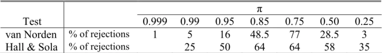
Although our testing strategy gives satisfactory results about detection of periodically collapsing rational bubbles, our main contribution is on the estimation of threshold level and probability of collapse. Detection of probability of collapse and threshold level for bubbles makes our study unique, because all of the papers considered so far try to determine if there is a bubble or not. None of them is interested in exposing these critical features of bubbles. However, since our testing method involves the estimation of threshold level, it also provides us to get an estimate of probability of collapse, because when one knows threshold level, it is not difficult to extract probability of collapse. The results of the simulations are given in the following table:

Table 15. Simulation Results π

0.99 0.95 0.85 0.75 0.50 0.25 Median of prob. of collapse 0.05

(0.01) 0.06 (0.05) 0.15 (0.15) 0.23 (0.25) 0.33 (0.50) 0.50 (0.75) Median of threshold level 12.70

(1.00) 1.62 (1.00) 1.09 (1.00) 1.17 (1.00) 1.09 (1.00) 0.59 (1.00) Median of ρ1 0.92 (1.05) (1.05) 1.00 (1.05) 1.03 (1.05) 1.05 (1.05) 1.04 (1.05) 1.00 Median of ρ2 1.02 (1.06) (1.10) 1.10 (1.23) 1.25 (1.40) 1.39 (2.10) 2.07 (4.20) 0.85

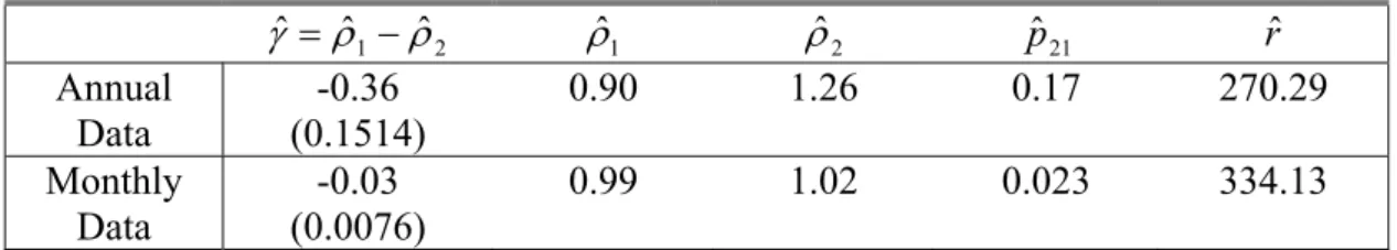
Note: The simulations are done with Pt as dependent and Rt threshold variable. True values are in the