Resolution of the ATLAS muon spectrometer monitored drift tubes in LHC Run 2

Journal of Instrumentation

OPEN ACCESS

Resolution of the ATLAS muon spectrometer monitored drift tubes in

LHC Run 2

To cite this article: The ATLAS collaboration 2019 JINST 14 P09011

2019 JINST 14 P09011

Published by IOP Publishing for Sissa Medialab Received: July 2, 2019 Accepted: August 22, 2019 Published: September 16, 2019

Resolution of the ATLAS muon spectrometer monitored

drift tubes in LHC Run 2

The ATLAS collaboration

E-mail:

atlas.publications@cern.ch

Abstract: The momentum measurement capability of the ATLAS muon spectrometer relies

funda-mentally on the intrinsic single-hit spatial resolution of the monitored drift tube precision tracking

chambers. Optimal resolution is achieved with a dedicated calibration program that addresses the

specific operating conditions of the 354 000 high-pressure drift tubes in the spectrometer. The

calibrations consist of a set of timing offsets and drift time to drift distance transfer relations, and

result in chamber resolution functions. This paper describes novel algorithms to obtain precision

calibrations from data collected by ATLAS in LHC Run 2 and from a gas monitoring chamber,

deployed in a dedicated gas facility. The algorithm output consists of a pair of correction constants

per chamber which are applied to baseline calibrations, and determined to be valid for the entire

ATLAS Run 2. The final single-hit spatial resolution, averaged over 1172 monitored drift tube

chambers, is 81.7 ± 2.2 µm.

Keywords: Gaseous detectors; Muon spectrometers; Particle tracking detectors (Gaseous

de-tectors); Wire chambers (MWPC, Thin-gap chambers, drift chambers, drift tubes, proportional

chambers etc)

2019 JINST 14 P09011

Contents

1

Introduction

1

2

ATLAS detector

2

3

Analysed data

3

4

MDT calibration

4

4.1 Drift radius determination

4

4.2 t

0

determination

4

4.3 R(t) function determination

5

4.4 Gas monitor chamber

6

4.5 Residuals and resolution

7

5

Correction algorithms

8

5.1 δt

0

correction

8

5.2 δP correction

10

6

Resolution results

13

7

Systematic uncertainties

15

8

Conclusion

16

The ATLAS collaboration

19

1

Introduction

This paper summarizes the calibration procedure and reports the single-hit spatial resolution of the

monitored drift tubes (MDT) in the ATLAS muon spectrometer (MS) during Run 2 of the Large

Hadron Collider (LHC), spanning the 2015–2018 operating period. In this context, single-hit refers

to the signal produced by a charged particle passing through a drift tube. The calibrations use data

from both the spectrometer MDT chambers and a dedicated gas monitor MDT chamber (GMC),

and are performed at the ATLAS muon calibration centers [

1

].

The MS design momentum resolution δp/p is ∼3% at 100 GeV and around 10% at 1 TeV [

2

],

allowing both Standard Model measurements and new physics searches in processes containing

high-momentum final-state muons [

3

]. Such searches may include the decay of heavy resonances

into high transverse momentum (p

_T

) muons, demanding superior spectrometer performance for

their discovery. For muons of p

_T

above 100 GeV, the drift tube single-hit resolution (and to a lesser

extent, the chamber alignment) becomes an important contribution to the transverse momentum

2019 JINST 14 P09011

resolution, and is the dominant factor above 250 GeV [

2

]. At high momentum, the p

_T

resolution

σp

_T

is determined by the relation σp

T

/p

T

∝

σ

res

× p

T

[

4

], where σres

is the single-hit spatial

resolution. The design resolution is σ

res

= 80 µm [

2

].

The objective of the MDT calibration program is to achieve this resolution for all 354 000 drift

tubes assembled into 1172 MDT chambers throughout all ATLAS data taking in LHC Run 2. The

primary MDT calibration ingredients consist of tube t

₀

timing offsets (referred to here as t

₀

offsets or

just t

₀

) and chamber-specific drift electron time to drift distance transfer relations, hereafter referred

to as R(t) functions. The t

₀

offset is primarily a function of cable length and electronics delays,

while the R(t) function depends on the gas properties.

The operating conditions of the MDT detectors in the ATLAS cavern are characterized by large

temperature gradients, occasional component faults, variations in humidity, background radiation,

flow, pressure and mixture instabilities of the gas supply, all of which affect the timing response. In

order to achieve the optimal resolution the calibration constants are routinely monitored, corrected

for many of these second-order effects, and updated.

This paper describes the algorithms which generate a pair of correction parameters for the

t

₀

offsets and the R(t) functions. These pairs of chamber-specific constants compensate for a

number of systematic uncertainties associated with the operating conditions of the MDT chambers.

As a final result, the MDT tube spatial resolution that has been achieved in ATLAS Run 2 is

presented. Unless otherwise noted, all reported errors are statistical.

2

ATLAS detector

The ATLAS experiment [

5

] at the LHC is a multipurpose particle detector with a forward-backward

symmetric cylindrical geometry and a near 4π coverage in solid angle.

1

It consists of an inner

track-ing detector (ID) surrounded by a thin superconducttrack-ing solenoid providtrack-ing a 2 T axial magnetic

field, electromagnetic and hadronic calorimeters, and a muon spectrometer. The ID covers the

pseu-dorapidity range |η| < 2.5. It consists of silicon pixel, silicon microstrip, and transition-radiation

tracking detectors. Lead/liquid-argon (LAr) sampling calorimeters provide electromagnetic (EM)

energy measurements with high granularity. A steel/scintillator-tile hadronic calorimeter covers the

central pseudorapidity range (|η| < 1.7). The endcap and forward regions are instrumented with

LAr calorimeters for EM and hadronic energy measurements up to |η| = 4.9.

The ATLAS muon spectrometer is cylindrical, 22 m in diameter and 45 m in length, surrounding

the calorimeters with an acceptance coverage of 2π in azimuth and ±2.7 in pseudorapidity. It

consists of a barrel and two endcap sections located in an air-core toroidal magnetic field generated

by eight coils for each section. The field integral of the toroids ranges between 2.0 and 6.0 T m

for most of the acceptance, while the field magnitude at the MDT chambers ranges from near zero

to 0.2 T in most of the endcap region (1.05 < |η| < 2.7), and averages about 0.6 T in the barrel

(|η| < 1.05) region [

2

]. The MS identifies muons, provides muon triggers and, integrating with the

1ATLAS uses a right-handed coordinate system with its origin at the nominal interaction point in the center of the detector and the z-axis along the beam pipe. The x-axis points from the interaction point to the center of the LHC ring, and the y-axis points upwards. Cylindrical coordinates (r, ϕ) are used in the transverse plane, ϕ being the azimuthal angle around the z-axis. The pseudorapidity is defined in terms of the polar angle θ as η = − ln tan(θ/2). The momentum in the transverse plane is denoted by p_T.

2019 JINST 14 P09011

inner detector information, measures their charge sign and momenta. The MDT chambers perform

precision charged-particle tracking in the plane defined by the beam axis (z) and the radial distance to

the beam (r). The momentum measurement is based on the track curvature in these r-z coordinates,

while resistive-plate chambers (RPC) and thin-gap chambers (TGC) provide triggering in the barrel

and endcaps respectively, and readout of the so called second coordinate in the r-ϕ non-bending

plane. The MDT chambers are assembled in three nested cylindrical barrel stations and three main

coaxial discs in each of the endcap regions. A fourth annulus of endcap chambers covers a limited

pseudorapidity region spanning from the barrel to the endcap. They are constructed of pairs of

close-packed multilayers of 3 cm diameter cylindrical aluminum drift tubes, 1 m to 6 m long for the

inner stations close to the beam and outer stations, respectively. Each multilayer comprises either

three or four single planes, depending on the barrel (endcap) chamber radial (Z-axis) position, with

each plane containing from 12 to 72 tubes. A 50 µm diameter anode wire is centered to within 30 µm

of the axis of a 1.46 cm (1.5 cm) inner (outer) radius aluminum tube. The MDT gas is a mixture of

93% Ar and 7% CO

₂

plus a few hundred ppm of water vapour at 3 bar pressure. The gas flows in

a common trunk line to distribution racks and is fed in parallel to all drift tubes at a rate of roughly

one tube volume per day. The total gas throughput to the entire MDT system is about 2×10

6

_L/day.

The tubes are operated at 3080 V anode voltage to deliver a gas avalanche amplification gain of

20 000. The single-hit efficiency for a minimum-ionizing particle is nearly 100% [

6

].

First-level triggers [

7

] are implemented in hardware and combine muon spectrometer and

calorimeter measurements to accept events at a maximum rate of 100 kHz. These first-level triggers

are followed by more refined software-based triggers that reduce the accepted event rate to 1 kHz

on average.

3

Analysed data

The results presented here are based on a subset of the ATLAS Run 2 proton-proton collision

data at a center-of-mass energy

√

s

= 13 TeV. Specifically, this analysis uses 1.3 fb

−1

of data that

were acquired in 2015, 23.8 fb

−1

_{in 2016, and 22.3 fb}

−1

_{in 2017. The 2015 and 2017 data include}

7.9 pb

−1

_{and 55.3 pb}

−1

_{, respectively, collected with the MS toroid magnet turned off. The data set is}

from the primary ATLAS physics data stream that includes all triggers and was processed with data

quality selections common to all physics analyses. The selected set of data runs is distributed along

the whole data acquisition period for each year, allowing checks of the stability of the parameters

under study in different conditions. Each single run contains enough muon tracks per chamber to

allow the determination of the R(t) and resolution functions. Two corrections that depend on the

non-bending plane second coordinate are applied to the time of the MDT signal by the offline event

reconstruction software: (1) the magnetic-field-induced Lorentz angle effect on the drift time [

8

]

and (2) the signal propagation time associated with the hit position along the wire.

This paper uses single-hit information from muon tracks with p

_T

> 20 GeV that are

recon-structed in the ID and MS. The data include drift times, drift radii and timing offsets as used by

the offline tracking reconstruction algorithms. A minimum of 1000 tube hits per chamber per run

is required to obtain stable fit results in the analysis. As a consequence of these selection criteria

the number of chambers for which results are obtained has a run-to-run variation of 0.3%. When

2019 JINST 14 P09011

possible, multiple consecutive runs with the same gas conditions are grouped together in order to

reach a minimum number of muon tracks per chamber.

4

MDT calibration

This section introduces the drift radius measurement and the basic calibration parameters necessary

for its determination. The operational definition of the single-hit spatial resolution as applied in

this analysis is then presented.

4.1

Drift radius determination

The MDT drift tube signal, or hit, provides the pulse arrival time, and a quantity reconstructed as the

collected electric charge of the signal pulse. Read-out is accomplished with 24-channel front-end

cards. These cards amplify, shape and discriminate the signals with programmable thresholds, then

digitize the data. The hit time data are recorded in 1.2 µs windows initiated by a first-level trigger

signal with a 0.78125 ns minimum digitization time. The charge contained in the leading edge of

the signal is stored as voltage on a capacitor and read out as a run-down time using the Wilkinson

technique [

9

].

The signal arrival time is relative to a specific proton-proton interaction time called the bunch

crossing identifier. The bunch crossing time is measured in 25 ns ticks synchronized with an LHC

global 40 MHz clock, and is subtracted in the read-out electronics hardware to yield the raw pulse

arrival time. This pulse arrival time includes, in addition to the drift time, several timing offsets: the

time-of-flight of the particle (muon) from the proton-proton interaction point to the tube, the signal

propagation time along the tube wire, plus various fixed electronics and cable latencies. The sum

of all these is referred to as the t

₀

offset. The t

₀

offset therefore represents the drift time produced

by a particle crossing at the tube wire.

The raw time for every hit is converted into a drift time by subtracting the tube time offset.

The drift time is a measure of the transit time of electrons generated by the primary ionization

and subsequent avalanche multiplication to arrive at the anode wire. The resultant drift time is

then mapped to the drift distance (circle) by means of a time-to-distance R(t) transfer function, an

example of which is shown in figure

1

. The best straight line tangent to all such drift circles in a

single chamber forms a track segment.

In ATLAS, the t

₀

offset is a property of a single tube, whereas an R(t) function is associated to a

single MDT chamber. This association is valid to the extent that the operating conditions are uniform.

Since chambers share a common high-voltage supply, gas pressure and thermal environment, these

conditions are generally met at the chamber level. These t

₀

offsets and R(t) functions, globally

called calibration constants, are generated by the ATLAS calibration computing centers.

4.2

t0

determination

While the t

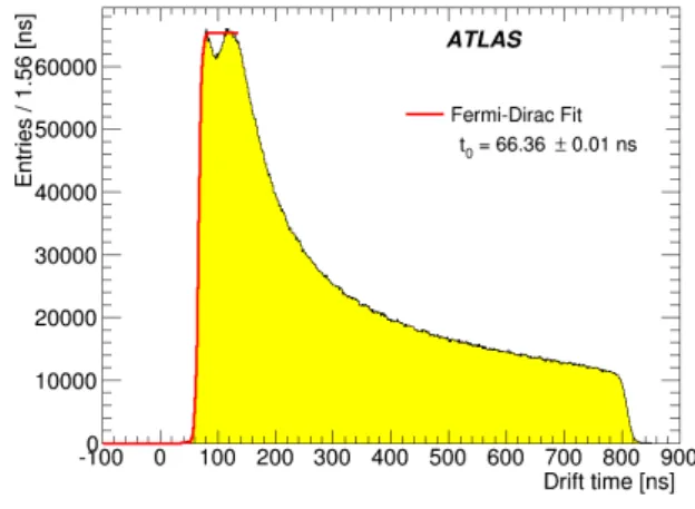
₀

offset represents the drift time of a hit at the wire, operationally it is defined as the

point of 50% of maximum amplitude of a Fermi-Dirac sigmoid function fit to the rising edge of an

MDT drift time spectrum [

10

], as illustrated in figure

2

. t

₀

offsets are nominally determined for all

tubes in the MS using single tube spectra or, when hit statistics are poor, the combined spectra from

groups of 24 equal-length tubes sharing a common readout card. This t

₀

offset definition is subject

2019 JINST 14 P09011

Figure 1.Gas monitor chamber R(t) function for

93% Ar-7% CO₂ (and less than 0.1% of water vapour) for standard condition: 293 K, 3080 V and 3 bar, obtained via autocalibration.

Figure 2. Measured drift time spectrum for a

generic MDT chamber with a Fermi-Dirac func-tion fit to the rising edge of the distribufunc-tion.

to small systematic uncertainties of order 1 ns. These arise from different data selection, different

background level and operating conditions in the GMC (see section

4.4

) and the MDT systems,

which affect the number of hits near the wire, the slope of the rising edge, and the subsequent fit

result. These systematic effects are relevant for the GMC-based universal R(t) function described

in section

4.3

which is computed using the GMC t

₀

offsets. They are resolved using a correction

parameter, δt

₀

, described in section

5.1

.

4.3

R(t) function determination

A standard method to extract the R(t) function is by an autocalibration algorithm [

11

]. This

algorithm, using a given set of t

₀

offsets, iterates the linear fit to the drift radii in a chamber,

each time updating the R(t) function until the residuals converge to a minimum. An autocalibration

R(t)

function is self-adapting to the chamber conditions, but a daily implementation of this procedure

for every single MDT chamber requires significant computing resources and a large amount of data

transfer and storage.

The alternative R(t) function calibration method used here adopts the temperature-corrected

universal R(t) (URT), where the URT is the GMC R(t) function derived using autocalibration for

standard operating conditions (defined as gas pressure 3 bar, high voltage 3080 V, temperature 293 K,

and GMC t

₀

offsets). The URT method assumes that the absolute measured values of the chamber

operating conditions of both the GMC and the MDT chambers are all known and that their differences

can be corrected. The main sources of systematic differences resulting from this assumption are:

• The MDT chamber pressures can differ from the 3 bar nominal point due to several factors:

local gas flow rates, pressure gauge location in the gas flow circuit, and pressure sensor

offsets. Furthermore, sensors used in the GMC and in the MDT gas racks have systematic

uncertainties of 10–20 mbar.

• The internal MDT gas temperature may be systematically misrepresented by the thermal

sensors. There are typically eight sensors mounted on the tube walls at different locations in

2019 JINST 14 P09011

the chamber. These sensors are read out periodically, and a daily average value over all sensors

is computed. However, due to possible thermal gradients across the chambers (on average

1.8 ± 0.7 (RMS) K), and because the sensors are external to the tubes, this average temperature

may not accurately represent the internal temperature everywhere in the gas volume.

• The actual high voltage supplied to chambers might deviate slightly (by about 1 V) from

the nominal 3080 V operating voltage, although this has an effect of less than 0.1% on the

maximum drift time. A larger high-voltage deviation generally indicates equipment failure,

not a systematic error, and it is addressed during the detector access periods.

To correct for these effects a single catch-all parameter, referred to as effective pressure, δP, is

defined. This parameter is used in a phenomenological correction function described in section

5.2

.

In summary, an MDT chamber requires two types of calibrations: an R(t) function and a set

of t

₀

offsets, each with a specific set of uncertainties. Two similar algorithms provide correction

factors that compensate for these uncertainties and lead to improved single-hit spatial resolution.

4.4

Gas monitor chamber

The GMC [

10

] is an independent MDT chamber that operates in the surface gas facility, outside of

the ATLAS experimental cavern. It has two gas partitions each independently sampling the common

MDT trunk supply and exhaust lines that serve the entire MDT system, and records cosmic-ray

muons at a rate of about 14 Hz. It is housed in a stable thermal enclosure where all operating

parameters, gas flow, pressure, temperature, and high voltage, are continuously monitored.

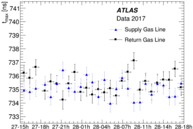
The principal GMC output is a measurement of the maximum drift time, t

_max

= t

_w

−t

₀

, where t

_w

is the arrival time of a hit located at the tube wall. A drift time spectrum, similar to figure

2

, is

com-puted for standard operating conditions by applying a correction function [

12

] based on the output

of chamber-mounted pressure and temperature sensors. The tail end of the spectrum is fitted using

a modified Fermi-Dirac sigmoid function similar to that used to obtain the t

₀

offsets, and the t

_max

is

defined as a fit parameter, as described in ref. [

10

]. The t

_max

is published hourly to the online run

monitoring system and to the muon calibration centers. A variation of t

_max

> 1 ns triggers the

calcu-lation of a new set of R(t) functions for the track reconstruction. The t

_max

is sensitive to small changes

in the gas composition: for example, a 100 ppm absolute increase in water vapour content yields

a nearly 7 ns increase in t

_max

[

13

]. A single 24-hour period of GMC t

_max

data is shown in figure

3

,

where the stability is better than 1 ns RMS. The GMC t

_max

superimposed with the same quantity

de-termined from the average of all chambers over the 2016 data-taking period is presented in figure

4

.

A one-time offset of −12 ns is applied to compensate for the typical difference in gas temperature

between the MDT and the standard URT that range from about 4.5 to 5 K. The range of t

_max

variation

over one year is 15 ns. This change, observed annually, is attributed to the seasonal variation in

am-bient humidity in the ATLAS cavern that modulates the content of water vapour in the gas mixture.

The GMC produces URT functions every two hours. After local GMC temperature and

pressure corrections are applied, the URT registers only changes in the gas composition. Based on

the daily average of measurements from detector-mounted thermal sensors, the URT is converted

into chamber-specific R(t) functions [

12

]. These chamber R(t) functions are further tuned by the

δP correction parameter, as detailed in section

5.2

.

2019 JINST 14 P09011

Figure 3. Hourly GMC measurements of

t_maxover a single day during Run 2.

Figure 4. Measurement of t_max daily average

over the entire 2016 data-taking period, obtained from an average of all chambers and from the GMC. The horizontal axis represents run num-bers, which are not uniformly distributed in time. Dotted lines delineate months.

4.5

Residuals and resolution

Track segments in a chamber are the best-fit straight lines tangent to the N circles defined by N drift

radii. The distance of closest approach of a hit radius to this fit line is either a fit or hit residual. The

former results when all N data points are included in the linear fit, and the latter is a measure of the

j

th

residual when the j

th

point is excluded from the fit of the other N − 1 points. Hit and fit residual

distributions (N entries per track, for all tracks in the analysed data set) are generated for each

MDT chamber. Residuals are calculated for each of 15 radial bins, 1 mm wide, from 0 to 15 mm

in drift radius r, as well as for a single 15-mm-wide radial bin. The former are used to obtain the

radial dependence of the resolution and the latter is used to obtain the single-hit spatial resolution,

both averaged over all tubes in a chamber. The residual distributions are fitted using a

double-Gaussian function as expressed in equation (

4.1

): this choice is dictated by the stochastic nature

of the signal formation that arises from ion-pair creation, gas diffusion and electron-ion transport

and, importantly, allows for the dependence of the drift velocity on drift radius, as indicated by the

non-linearity of the R(t) function in figure

1

. These properties produce residual distributions with

radially dependent widths, including tails that are attributed to misassociated track hits from

delta-rays and asynchronous background hits. While a single-Gaussian function inadequately describes

the distributions for all radial bins, the double-Gaussian function used here provides a good fit to

the residuals with a minimal increase in the number of free parameters. The fit function is:

f (r)

= A

_n

e

−(r −¯r)2 2σ2n

_{+ A}

_w

_e

−(r −¯r)2

2σ2w

,

(4.1)

where A

_n

, A

_w

, σ

_n

, σ

_w

are the amplitudes and standard deviations of a narrow and a wide Gaussian

component. The two terms in equation (

4.1

) are constrained to a common mean ¯r, and fit over a

residual range of ± 0.5 mm, which contains more than 99% of hits (section

7

). The σ parameters

(for fit and hit residuals) are determined for the r

th

_{radial bin of the amplitude-weighted standard}

2019 JINST 14 P09011

deviations of the double-Gaussian function by:

σ(r) =

A

n

(r)σ

n

(r)

+ A

w

(r)σ

w

(r)

A

_n

(r)

+ A

_w

(r)

.

(4.2)

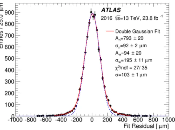
where the dependence of the fit parameters on the drift radius is explicitly indicated. Fit and

hit residual distributions for a representative chamber at a drift radius near the wire, where the

resolution is broader than far away from the wire, are shown in figures

5

and

6

, respectively. These

distributions are fit with the function of equation (

4.1

). For comparison purposes a single-Gaussian

fit within the FWHM of these distributions is also shown.

Figure 5.Fit residual distribution for a

represen-tative chamber for the radial bin r = [2, 3] mm. A double-Gaussian (solid line) is fit in the range ±0.5 mm. A single-Gaussian (dotted line) is fit within the FWHM but shown out to ±0.5 mm.

Figure 6. Hit residual distribution for the same

chamber and radial bin as in figure5.

The drift tube spatial resolution, σ

_res

, is the geometric mean of the fit and hit residual widths [

14

]

defined as:

σ

_res

(r)

=

pσ

_fit

(r) ·

σ

_hit

(r)

(4.3)

This approach was checked by Monte Carlo simulation. About 10

6

_{tracks incident on a generic}

chamber within a 10

◦

_{angular range were generated. The drift radii assigned to these tracks were}

Gaussian distributed about their initial values using a radially dependent input resolution function

derived from a test beam [

15

]. These smeared hit points were linearly fit and the output resolution

for each radial bin was obtained using equation (

4.3

). The mean difference over the tube radius

between the output and input resolution is 0.3 ± 0.2 µm, confirming the validity of the formulation.

5

Correction algorithms

This section describes the algorithms used to determine the δt

₀

and δP corrections and their

associated metrics, the track residuals and the resolution.

5.1

δt0

correction

The default t

₀

offset definition may vary by the order of 1 ns from the t

₀

value that provides the best

resolution. The algorithm described here is a variant of the tuning procedures designed to find the

2019 JINST 14 P09011

best linear fit to a track segment by tuning the t

₀

on a track-by-track basis [

16

]. The δt

₀

correction

method instead optimizes the default t

₀

by testing a new, modified t

₀

associated with a single

chamber simultaneously for all tubes and for all tracks in a data run, while keeping the R(t) function

fixed. The algorithm operates on track segments containing at least as many hits as there are drift

tube layers in the chamber, i.e. a minimum of six (eight) hits for a six-layer (eight-layer) chamber.

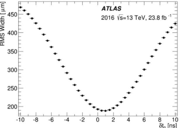
The procedure steps through δt

₀

over a range of ±10 ns in 0.5 ns steps. At each step, new drift times

and drift radii are computed and the segments are re-fit. Importantly, the residuals are evaluated

only for hits with drift radii r < 5 mm where the drift velocity is largest, about 50 µm/ns. By using

only these near-wire residuals the procedure is practically insensitive to the R(t) function and avoids

compensating for systematic uncertainties which come into play at larger drift radii (see figure

12

).

Figure 7. Hit residual distributions for a

repre-sentative chamber for t₀correction parameter set to −4 ns (left), +1 ns (center) and +6 ns (right) from the default value. Widths are 296, 188 and 303 µm, respectively.

Figure 8. Typical RMS widths of hit residual

distributions of hits less than 5 mm from the wire as a function of the t₀ correction, for the same chamber as in figure7.

Figure

7

shows segment hit residuals from the t

₀

correction procedure for a representative

chamber for δt

₀

values of −4, +1, and +6 ns. Figure

8

shows the incremental change with each

step of the residual RMS widths for the entire range of δt

₀

values relative to the initial t

₀

. The

optimal δt

₀

is the one yielding the minima of the RMS widths of the fit and hit residual distributions.

The value on the vertical axis corresponding to the minimum in figure

8

does not represent the

resolution, but only the RMS spread of the hit residuals near the wire.

2

The δt

₀

correction procedure is applied to 2015 data (the first year of Run 2 operation) using

initial t

₀

offsets generated by the MDT calibration centers. The δt

₀

corrections obtained in a much

higher peak-luminosity November 2015 run, 4.8 × 10

33

_cm

−2

_s

−1

_{, are shown in figure}

₉

_{, which}

reveals an average t

₀

global correction of 1.3 ns with a RMS spread of 0.7 ns. The tails of the

distribution are populated by a few chambers that were measured to have been constructed with

structural non-conformities affecting the internal alignment of the tubes and therefore of the hit

positions. The δt

₀

correction tries to compensate for this misalignment.

2For over 95% of the MDT chambers the double-Gaussian fits yield the same t₀minima as obtained using the RMS of the residual distributions. In the remaining chambers the fit method can lead to anomalous minima, so for consistency and stability of the results, the RMS method to establish the minimum is adopted for all chambers.

2019 JINST 14 P09011

Figure 9. Distribution of δt₀ for one run in

November 2015 determined by the t₀ correction algorithm.

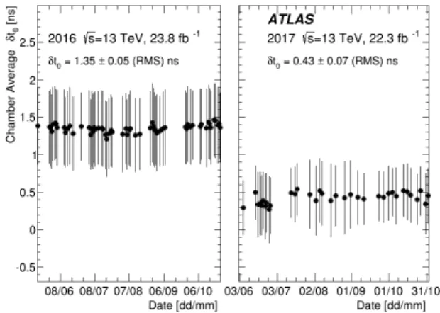
Figure 10. Chamber-averaged δt₀values for runs

in 2016 (left) and 2017 (right). Uncertainties are the RMS of the distributions.

The determination of the δt

₀

corrections for all MDT chambers was repeated for a selection of

data runs that span all data-taking periods in 2016 and 2017. The chamber-averaged δt

₀

corrections

for each run are shown in figure

10

. At least 1165 out of the total 1172 chambers are included in

each data point used for this average, depending on the integrated luminosity of the run. For the 65

runs analysed in 2016 the mean global δt

₀

offset is 1.35 ± 0.05 (RMS) ns, consistent with the result

determined from the 2015 data set. The δt

₀

corrections from 2016 are then added to the calibration

constants for 2017, so that the algorithm, when applied to the 2017 data set, produces a smaller

global shift with a mean of 0.43 ± 0.07 (RMS) ns.

Figure

11

shows the chamber-by-chamber δt

₀

difference between the first and last runs of the

2017 data set. In the first run, the toroid magnetic field was off and in the last run the field was at

full strength and the instantaneous luminosity was higher by one order of magnitude. The mean

difference is consistent with zero. This result demonstrates that the δt

₀

parameter, once established,

remains stable for all chambers over a large range of instantaneous luminosity and is insensitive to

the magnetic field.

5.2

δP correction

Optimization of the R(t) functions is done with an effective pressure parameter, δP, that corrects

for the (small) inaccuracies in gas pressure sensors, temperature measurement, and high voltage.

In all three cases, minor variations from nominal values produce radially dependent changes in the

R(t)

function, such that a single, scalable correction function can be used. The calculation of this

function is done using the Garfield program [

17

] configured to model the drift electron transport

in MDT tubes with standard operating parameters as in section

2

. Specifically, a pure Ar-CO

2

gas

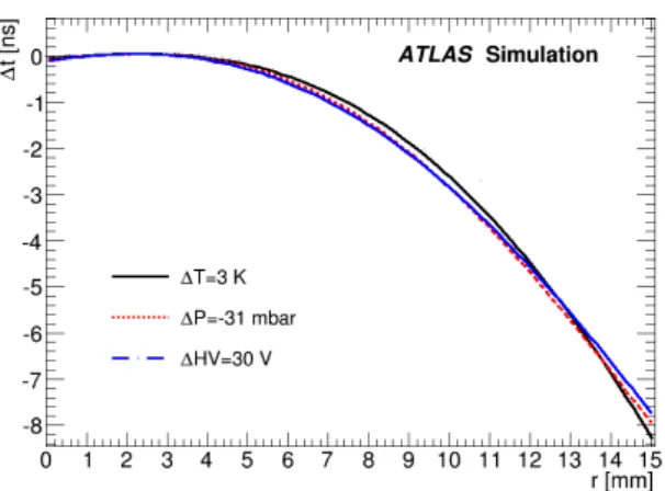
mixture without water vapour and zero magnetic field is used. Figure

12

shows the predicted change

in the drift time as a function of drift radius for variations of temperature, pressure and high voltage

from their reference values. This drift time response was previously validated with temperature

data [

12

]. The maximum effect on the drift time is at the tube wall as expressed in equation (

5.1

),

where the temperature correction is −2.6 ns/K, while the pressure correction function scales as

−

0.1 K/mbar relative to the temperature correction. The negative sign means that an increase in gas

2019 JINST 14 P09011

Figure 11. Chamber-by-chamber difference in

the δt₀ parameter obtained from the June (toroid magnetic field off) and November (toroid mag-netic field on) 2017 data.

Figure 12. Garfield simulation of drift time

vari-ation as a function of drift radius for: +3 K, −31 mbar, and +30 V change relative to 293 K, 3 bar and 3080 V, respectively.

pressure at fixed temperature corresponds to an increase in gas density, a decreased drift electron

mean free path, and thus longer drift times. Similarly, a higher voltage at fixed pressure leads to

an increased electric field and higher drift velocity. Importantly, for any of these parameters, the

curves in figure

12

indicate a negligible effect on drift times for radii smaller than 5 mm. For

small deviations of the high voltage from the nominal setting, the drift time changes by only about

0.26 ns/V at the tube wall, thus typical systematic offsets of 1 V have a negligible effect:

∆t(

wall) [ns] = −2.6

ns

K

× ∆T [

K] = +0.26

ns

mbar

× ∆P [

mbar] = −0.26

ns

V

× ∆V [

V].

(5.1)

The effective pressure correction algorithm is similar to the δt

₀

method and uses the same

track-segment hit selection. For a collection of track-track-segment hits, δP is incremented in 5 mbar steps

through a ±100 mbar range of test pressures centered around the nominal 3 bar. The R(t) function is

recalculated using the correction function shown in figure

12

rescaled by the P+δP effective pressure

value assumed in the scan, new drift radii are obtained from the newly corrected R(t) function, and

track segments are re-fit and residuals evaluated. The procedure is initiated with the set of

chamber-specific R(t) functions of the day of the run. The δt

₀

corrections found previously are applied to

the hit drift times. For δP determination, the residuals are calculated for all drift radii.

Similar to the δt

₀

procedure, the optimal δP is the one yielding the minimum of the RMS width

of the fit and hit residual distributions. The hit residuals for three δP values, of −40 mbar, 10 mbar

and 60 mbar, are shown for a representative chamber in figure

13

. Figure

14

shows the RMS width

of the hit residual distribution as a function of δP for the full scan range. The minimum at 10 mbar

represents the best value of this parameter.

The minima of curves similar to figure

14

, taken as the δP step corresponding to the lowest

residual, were initially determined for all MDT chambers using data from August 2015 with the

toroid magnet turned off. The algorithm was applied to a set of collision runs acquired 2.5 months

later with the magnetic field turned on, and with 25 times higher instantaneous luminosity (from

0.17 × 10

33

_cm

−2

_s

−1

_{in mid August to 4.8 × 10}

33

_cm

−2

_s

−1

_{at beginning of November), yielding in}

both cases an average correction δP of 30.0 ± 0.3 mbar with an 11 mbar RMS spread. Distributions

2019 JINST 14 P09011

Figure 13. Fit residual distributions for a

repre-sentative MDT chamber for δP = −40 mbar (left), +10 mbar (middle, optimal setting) and +60 mbar (right). RMS widths are 141, 131 and 144 µm, respectively.

Figure 14. Fit residual RMS as a function of

δP for the same chamber as in figure13.

of the latter δP results are shown in figure

15

, and the chamber-by-chamber differences in the

δP correction for the two data sets are shown in figure

16

. The measured change is within the

δP step size. The corrections are stable in time and insensitive to both the magnetic field and the

increased hit rates that result from higher instantaneous luminosity.

Figure 15. Distribution of δP for a

high-luminosity run in November 2015.

Figure 16. Chamber-by-chamber difference of

δP for a run with the toroidal magnetic field off and a run 2.5 months later with 25 times higher luminosity and the toroid on.

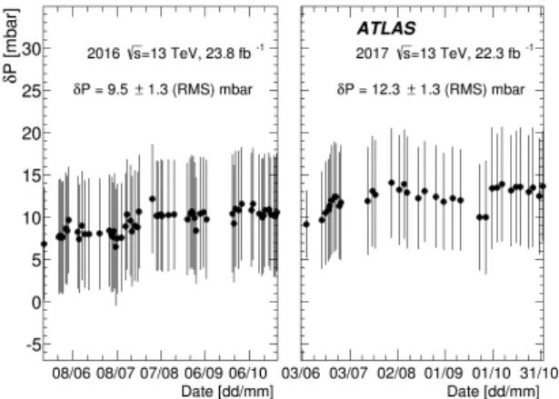
The δP algorithm was further applied to 65 collision runs acquired from May to October

2016, where the peak luminosity exceeded 10

34

_cm

−2

_s

−1

_{, more than twice that of November 2015.}

These runs used R(t) functions which included the δP corrections determined in the 2015 data.

The chamber-averaged δP value for each of the runs in 2016 and 2017 is shown in figure

17

as a

function of run date. The average of δP over all of 2016 data is 9.5 ± 0.8 mbar (RMS = 1.3 mbar)

and for 2017 is 12.3 ± 1.0 mbar (RMS = 1.3 mbar). The δP correction is stable over each year

to better than 3 mbar. Figure

18

shows the distribution of the chamber-by-chamber δP difference

2019 JINST 14 P09011

between the first and last runs in the 2016 data set. The mean difference is 2.3 ± 4.5 (RMS) mbar,

within the systematic uncertainty of the algorithm (section

7

). This overall result supports the initial

hypothesis that δP represents primarily systematic offsets of pressure gauges and other sensors and,

once determined, would remain stable throughout a year of running.

Figure 17. Chamber-averaged δP for each

anal-ysed run in 2016 (left) and 2017 (right). The un-certainties are the RMS spread of the chamber’s δP distribution.

Figure 18. Chamber-by-chamber differences in

δP between the first and last 2016 analysed run.

6

Resolution results

The single-hit MDT tube spatial resolution, as defined in equation (

4.3

), is measured in runs with

the toroidal magnetic field on. A requirement of p

_T

> 20 GeV for the muon transverse momentum

measured with the ID is applied to reduce the track curvature such that track segments could be

reliably fit with a linear function, even in the chambers in a high magnetic field. For these tracks the

negligible effects of the curvature due to magnetic field are folded into the systematic uncertainty.

The resolution obtained for a series of runs in each year of Run 2 is reported in figure

19

. The

full circles are calculated directly from fits to the default reconstructed track segments using the

standard t

₀

and R(t) calibration constants. The triangles include the δt

₀

corrections, and the blue

inverted triangles also include δP corrections. Significant improvements to the resolution in 2015

are the result of a first implementation of the corrections, dominated by δP. These δP corrections

were subsequently included in the standard production of R(t) function calibration constants. The

application of the procedure in each year yields 1–2 µm better resolution. The δt

₀

corrections in 2015

and 2016 each lead to a 3–4 µm improvement in resolution. From the beginning of 2017 the previous

year’s δt

₀

corrections are also applied, but only the δP corrections from 2016 (not those from 2015).

However, they yield an improvement of only 1.2 µm as shown in the right panel of figure

19

.

Both the best δt

₀

and δP values are incorporated in the end-of-year data reprocessing in order

to provide the best calibrated data for subsequent physics analyses.

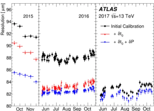
Figure

20

summarizes the resolution averaged over all runs in 2015, 2016, and 2017, for each

MDT chamber. The left panels show the initial resolutions obtained with the standard calibrations.

The right panels show the resolutions after all δt

₀

and δP corrections are implemented and using

2019 JINST 14 P09011

Figure 19. Resolution averaged over chambers

for runs in 2015 (left), 2016 (center) and 2017 (right) using default calibrations, with δt₀ and δP corrections. The initial calibration data in the right panel already include the δt₀corrections from 2016; additional δt₀correction is not needed.

Figure 20. Single-hit resolutions for each

cham-ber. Left: with default calibrations (different con-ditions every year). Right: with all corrections and most up-to-date R(t) functions.

daily updated R(t) functions: 84.9 ± 0.2 µm for 2015, 82.3 ± 0.2 µm for 2016, and 81.7 ± 0.2 µm

for 2017. Notably the improvements are measured both by the decrease of the mean value of the

distribution and by the decrease of the RMS width, indicating greater uniformity of the resolutions

of the whole ensemble of MDT chambers. In 2015, the δP corrections were applied for the first

time in Run 2, and then incorporated into the default calibrations for 2016. In 2016, the larger data

set allowed a much higher fraction of the initial t

₀

offsets to be determined for single tubes by the

calibration centers, resulting in a better overall initial resolution. The δt

₀

corrections from 2016 were

propagated into the default calibrations for 2017. For this reason, the incremental improvement in

both the mean and the RMS spread decreases with each year and the standard offline tube resolution

approaches the fully corrected result.

The final MDT drift tube spatial resolution, with all corrections described in previous sections

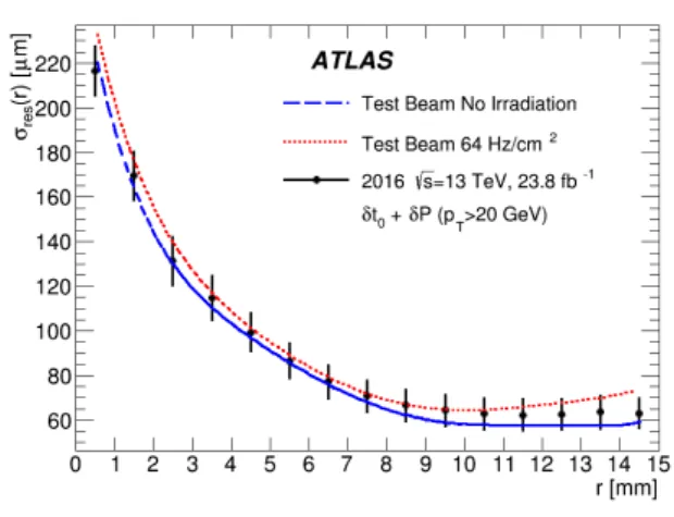
included, is shown as a function of drift radius in figure

21

and in figure

22

. In particular, figure

21

shows for 2016 the run-averaged resolution distributions σres

(r)

in 1 mm radial bins, where each

histogram bin entry represents a single chamber. This set of histograms therefore represents the full

range of resolution functions obtained for the entire ensemble of MDT chambers. The mean values

of these distributions are plotted as a single resolution function in figure

22

, where the uncertainties

are the RMS widths of the distributions for all chambers. For comparison, the resolution curves of a

single MDT chamber deployed in a test beam [

15

], with and without background irradiation, are also

displayed. The 2016 chamber-weighted resolution averaged over all radial bins is 86.4 ± 0.2 µm and

the average excluding the radial bin closest to the wire is 79.7 ± 0.2 µm. These two values bracket

the final 2016 resolution averaged over all chambers, presented in figure

20

, of 82.3 ± 0.2 µm.

Specific high instantaneous luminosity collision runs are analysed in order to measure the drift

tube rates by counting all chamber hits occurring within the MDT read-out time window of 1.2 µs

initiated by any muon trigger. This total number of hits per time window is normalized to the

total tube area to obtain a rate per unit area. These rates are consistently less than 10 Hz/cm

2

_,

2019 JINST 14 P09011

except for one set of 16 endcap inner chambers at high pseudorapidity whose rates range from

20 to 50 Hz/cm

2

_{, and another set of 16 chambers nearest the beam-line where rates range from}

60 to 140 Hz/cm

2

_{. At background rates above 100 Hz/cm}

2

_{, some loss in tracking efficiency and}

resolution is expected due to increased read-out electronics dead time and space charge in the gas,

respectively. Furthermore, an increase of the read-out electronics dead time was observed in special

high instantaneous luminosity runs at the end of Run 1, and addressed in Run 2 by optimizing the

data acquisition parameters. The resolutions from the analysed runs recorded in 2017 are entirely

consistent with the results from 2016 shown here.

Figure 21. Distribution of resolutions in 1 mm

radial bins of drift radius for all MDT chambers, averaged over all analysed runs from 2016.

Figure 22.Resolution as a function of drift radius

averaged over all MDT chambers and all analysed runs from 2016. Muon test-beam resolutions of an MDT chamber with background radiation from 0 to 64 Hz/cm2_{are also shown for comparison [15].} Uncertainties are RMS widths of the resolution distribution for all chambers.

7

Systematic uncertainties

The main sources of systematic uncertainty affecting the determination of the MDT resolution are:

(1) the fit uncertainty associated with the range of the double-Gaussian fit; (2) the use of linear fits

for curved track segments; (3) the precision of the δt

₀

and δP determinations; and (4) the accuracy

of equation (

4.3

) to describe the resolution. They are described in this section.

A double-Gaussian function is fit in a range of ±500 µm for both the fit and hit residual

distributions. This fit function matches well the central region with a narrow component and the

tails with the wider component. The fraction of hits included in the residual distributions exceeds

99% for most drift radii, and (95–97)% for the first millimeter nearest the wire. The reason for this

additional loss is attributed to the minimum 1 mm path length corresponding to the MDT front-end

electronics threshold of 23 primary ionization electrons [

9

]. For radial distances below 1 mm,

2019 JINST 14 P09011

the precision of the drift radius determination deteriorates due to the small number of ion pairs,

increasing the fraction of large residuals. A modification of the fit range down to ±400 µm and up

to ±1 mm produces an overall systematic variation in the resolution of 1 µm.

The path of a low-p

_T

muon track is slightly deflected by the magnetic field as it passes through

a chamber. For this reason, the tracks used in the analysis have a minimum transverse momentum

of 20 GeV, yielding an average p

_T

of 40 GeV. The systematic resolution broadening from using a

linear fit is determined from a Monte Carlo calculation using a worst-case 0.6 T magnetic field and

for the most prevalent MDT geometry: a six-layer chamber with a 17 cm spacer frame separating

the two multilayers. The hits are smeared with the nominal 80 µm resolution, linearly fit to generate

residuals, and the resolution computed from equation (

4.3

). The average resolution for p

_T

= 40 GeV

muons is broadened by about 2 µm relative to the nominal value. In addition, this uncertainty

from track curvature in the magnetic field is also directly investigated by comparing the resolutions

obtained with and without the toroidal magnetic field. The average resolution of all chambers with

the toroid field off is σ

off

= 80.1 ± 0.2 µm. The average broadening of the measured resolution due

to the toroidal field is 1.6 ± 0.3 µm, consistent with the result from Monte Carlo calculation.

The step of the correction algorithm is 0.5 ns for δt

₀

and 5 mbar for δP. The minima are found

separately for the hit and fit residual distributions, and agree to within one step for more than 90% of

the chambers. Therefore, the precision with which the parameters can be reliably established is

esti-mated to be half of the step size. The uncertainty for each parameter is determined by altering the

op-timal δt

₀

and δP values within ±0.25 ns for δt

₀

and ±2.5 mbar for δP and recalculating the resolution

functions. The average systematic uncertainty in the correction parameter determination is 1 µm.

A final, small systematic uncertainty derives from the accuracy to which the resolution function

of equation (

4.2

) reproduces the true resolution. This uncertainty, described in section

4.5

, is 0.3 µm.

The total systematic error of the single-hit spatial resolution measurement, taken as the sum in

quadrature of all contributions, is 2.2 µm, as summarized in table

1

, and about 2.6% of the overall

average resolution.

Table 1.Main resolution systematic uncertainties averaged over all chambers.

Systematic uncertainty

Size [µm]

Double-Gaussian fit range

1.0

Straight-line track fit

1.6

Optimal δP and δt

₀

values

1.0

Resolution function accuracy

0.3

Total

2.2

8

Conclusion

This document describes a novel method to optimize the single-hit spatial resolution of the muon

MDT chambers of the ATLAS experiment during Run 2 of the LHC. This method tunes the initial

t

₀

derived from drift time spectra and provides a correction parameter for R(t) functions produced

2019 JINST 14 P09011

by a gas monitor MDT chamber. The extracted corrections were used in the 2015 and 2016

end-of-year data reprocessing, and became fully integrated in the online calibrations from 2017

onward, yielding results consistent with those presented here. These two combined correction

parameters are shown to be very stable over a year, insensitive to increasing luminosity, variations

in environmental conditions, or the magnetic field. The method applied to the 2017 data achieves

a mean single-hit spatial resolution of 81.7 ± 0.2 ± 2.2 (sys) µm with an RMS spread of 7 µm over

all 1172 MDT chambers in the spectrometer. The resolution approaches the design value of 80 µm,

consistent over all MDT chambers, and stable across all run periods.

Acknowledgments

We thank CERN for the very successful operation of the LHC, as well as the support staff from our

institutions without whom ATLAS could not be operated efficiently.

We acknowledge the support of ANPCyT, Argentina; YerPhI, Armenia; ARC, Australia;

BMWFW and FWF, Austria; ANAS, Azerbaijan; SSTC, Belarus; CNPq and FAPESP, Brazil;

NSERC, NRC and CFI, Canada; CERN; CONICYT, Chile; CAS, MOST and NSFC, China;

COL-CIENCIAS, Colombia; MSMT CR, MPO CR and VSC CR, Czech Republic; DNRF and DNSRC,

Denmark; IN2P3-CNRS, CEA-DRF/IRFU, France; SRNSFG, Georgia; BMBF, HGF, and MPG,

Germany; GSRT, Greece; RGC, Hong Kong SAR, China; ISF and Benoziyo Center, Israel; INFN,

Italy; MEXT and JSPS, Japan; CNRST, Morocco; NWO, Netherlands; RCN, Norway; MNiSW

and NCN, Poland; FCT, Portugal; MNE/IFA, Romania; MES of Russia and NRC KI, Russian

Fed-eration; JINR; MESTD, Serbia; MSSR, Slovakia; ARRS and MIZŠ, Slovenia; DST/NRF, South

Africa; MINECO, Spain; SRC and Wallenberg Foundation, Sweden; SERI, SNSF and Cantons of

Bern and Geneva, Switzerland; MOST, Taiwan; TAEK, Turkey; STFC, United Kingdom; DOE and

NSF, United States of America. In addition, individual groups and members have received

sup-port from BCKDF, CANARIE, CRC and Compute Canada, Canada; COST, ERC, ERDF, Horizon

2020, and Marie Skłodowska-Curie Actions, European Union; Investissements d’ Avenir Labex

and Idex, ANR, France; DFG and AvH Foundation, Germany; Herakleitos, Thales and Aristeia

programmes co-financed by EU-ESF and the Greek NSRF, Greece; BSF-NSF and GIF, Israel;

CERCA Programme Generalitat de Catalunya, Spain; The Royal Society and Leverhulme Trust,

United Kingdom.

The crucial computing support from all WLCG partners is acknowledged gratefully, in

particu-lar from CERN, the ATLAS Tier-1 facilities at TRIUMF (Canada), NDGF (Denmark, Norway,

Swe-den), CC-IN2P3 (France), KIT/GridKA (Germany), INFN-CNAF (Italy), NL-T1 (Netherlands), PIC

(Spain), ASGC (Taiwan), RAL (U.K.) and BNL (U.S.A.), the Tier-2 facilities worldwide and large

non-WLCG resource providers. Major contributors of computing resources are listed in ref. [

18

].

References

[1] T. Dai et al., The ATLAS MDT remote calibration centers,J. Phys. Conf. Ser. 219(2010) 022028. [2] ATLAS collaboration, ATLAS muon spectrometer: technical design report,CERN-LHCC-97-022,

2019 JINST 14 P09011

[3] ATLAS collaboration, Search for new high-mass phenomena in the dilepton final state using 36 fb−1 of proton-proton collision data at√s= 13 TeV with the ATLAS detector,JHEP 10(2017) 182 [arXiv:1707.02424].

[4] ATLAS collaboration, Muon reconstruction efficiency and momentum resolution of the ATLAS experiment in proton-proton collisions at√s= 7 TeV in 2010,Eur. Phys. J. C 74(2014) 3034 [arXiv:1404.4562].

[5] ATLAS collaboration, The ATLAS experiment at the CERN Large Hadron Collider,2008 JINST 3 S08003.

[6] ATLAS collaboration, Commissioning of the ATLAS muon spectrometer with cosmic rays,Eur. Phys. J. C 70(2010) 875[arXiv:1006.4384].

[7] ATLAS collaboration, Performance of the ATLAS trigger system in 2015,Eur. Phys. J. C 77(2017) 317[arXiv:1611.09661].

[8] S. Horvat et al., Operation of the ATLAS muon drift-tube chambers at high background rates and in magnetic fields,IEEE Trans. Nucl. Sci. 53(2006) 562.

[9] Y. Arai et al., ATLAS muon drift tube electronics,2008 JINST 3 P09001.

[10] D.S. Levin et al., Drift time spectrum and gas monitoring in the ATLAS muon spectrometer precision chambers,Nucl. Instrum. Meth. A 588(2008) 347.

[11] C. Bacci et al., Autocalibration of high precision drift tubes,Nucl. Phys. Proc. Suppl. B 54(1997) 311. [12] N. Amram et al., Streamlined calibrations of the ATLAS precision muon chambers for initial LHC

running,Nucl. Instrum. Meth. A 671(2012) 40[arXiv:1103.0797].

[13] N. Amram et al., Gas performance of the ATLAS MDT precision chambers,IEEE Nucl. Sci. Symp. Conf. Rec.(2008) 3213.

[14] R.K. Carnegie et al., Resolution studies of cosmic ray tracks in a TPC with GEM readout,Nucl. Instrum. Meth. A 538(2005) 372[physics/0402054].

[15] M. Deile et al., Performance of the ATLAS precision muon chambers under LHC operating conditions,Nucl. Instrum. Meth. A 518(2004) 65[arXiv:1604.00236].

[16] P. Branchini, F. Ceradini, S.D. Luise, M. Iodice and F. Petrucci, Global time fit for tracking in an array of drift cells: the drift tubes of the ATLAS experiment,IEEE Trans. Nucl. Sci. 55(2008) 620. [17] R. Veenhof, Garfield, a drift-chamber simulation program, CERN program library entry W5050,

CERN, Geneva, Switzerland (1993).

[18] ATLAS collaboration, ATLAS computing acknowledgements,ATL-GEN-PUB-2016-002, CERN, Geneva, Switzerland (2016).

2019 JINST 14 P09011

The ATLAS collaboration

G. Aad101_{, B. Abbott}128_{, D.C. Abbott}102_{, O. Abdinov}13,∗_{, A. Abed Abud}70a,70b_{, K. Abeling}53_,

D.K. Abhayasinghe93_{, S.H. Abidi}167_{, O.S. AbouZeid}40_{, N.L. Abraham}156_{, H. Abramowicz}161_{, H. Abreu}160_, Y. Abulaiti6_{, B.S. Acharya}66a,66b,n_{, B. Achkar}53_{, S. Adachi}163_{, L. Adam}99_{, C. Adam Bourdarios}132_,

L. Adamczyk83a_{, L. Adamek}167_{, J. Adelman}121_{, M. Adersberger}114_{, A. Adiguzel}12c,ai_{, S. Adorni}54_, T. Adye144_{, A.A. Affolder}146_{, Y. Afik}160_{, C. Agapopoulou}132_{, M.N. Agaras}38_{, A. Aggarwal}119_, C. Agheorghiesei27c_{, J.A. Aguilar-Saavedra}140f,140a,ah_{, F. Ahmadov}79_{, W.S. Ahmed}103_{, X. Ai}18_, G. Aielli73a,73b_{, S. Akatsuka}85_{, T.P.A. Åkesson}96_{, E. Akilli}54_{, A.V. Akimov}110_{, K. Al Khoury}132_, G.L. Alberghi23b,23a_{, J. Albert}176_{, M.J. Alconada Verzini}88_{, S. Alderweireldt}36_{, M. Aleksa}36_, I.N. Aleksandrov79_{, C. Alexa}27b_{, D. Alexandre}19_{, T. Alexopoulos}10_{, A. Alfonsi}120_{, M. Alhroob}128_, B. Ali142_{, G. Alimonti}68a_{, J. Alison}37_{, S.P. Alkire}148_{, C. Allaire}132_{, B.M.M. Allbrooke}156_{, B.W. Allen}131_, P.P. Allport21_{, A. Aloisio}69a,69b_{, A. Alonso}40_{, F. Alonso}88_{, C. Alpigiani}148_{, A.A. Alshehri}57_,

M. Alvarez Estevez98_{, D. Álvarez Piqueras}174_{, M.G. Alviggi}69a,69b_{, Y. Amaral Coutinho}80b_{, A. Ambler}103_, L. Ambroz135_{, C. Amelung}26_{, D. Amidei}105_{, S.P. Amor Dos Santos}140a_{, S. Amoroso}46_{, C.S. Amrouche}54_, F. An78_{, C. Anastopoulos}149_{, N. Andari}145_{, T. Andeen}11_{, C.F. Anders}61b_{, J.K. Anders}20_,

A. Andreazza68a,68b_{, V. Andrei}61a_{, C.R. Anelli}176_{, S. Angelidakis}38_{, A. Angerami}39_,

A.V. Anisenkov122b,122a_{, A. Annovi}71a_{, C. Antel}61a_{, M.T. Anthony}149_{, M. Antonelli}51_{, D.J.A. Antrim}171_, F. Anulli72a_{, M. Aoki}81_{, J.A. Aparisi Pozo}174_{, L. Aperio Bella}36_{, G. Arabidze}106_{, J.P. Araque}140a_,

V. Araujo Ferraz80b_{, R. Araujo Pereira}80b_{, C. Arcangeletti}51_{, A.T.H. Arce}49_{, F.A. Arduh}88_{, J-F. Arguin}109_, S. Argyropoulos77_{, J.-H. Arling}46_{, A.J. Armbruster}36_{, A. Armstrong}171_{, O. Arnaez}167_{, H. Arnold}120_, A. Artamonov111,∗_{, G. Artoni}135_{, S. Artz}99_{, S. Asai}163_{, N. Asbah}59_{, E.M. Asimakopoulou}172_{, L. Asquith}156_, K. Assamagan29_{, R. Astalos}28a_{, R.J. Atkin}33a_{, M. Atkinson}173_{, N.B. Atlay}151_{, H. Atmani}132_{, K. Augsten}142_, G. Avolio36_{, R. Avramidou}60a_{, M.K. Ayoub}15a_{, A.M. Azoulay}168b_{, G. Azuelos}109,ax_{, M.J. Baca}21_,

H. Bachacou145_{, K. Bachas}67a,67b_{, M. Backes}135_{, F. Backman}45a,45b_{, P. Bagnaia}72a,72b_{, M. Bahmani}84_, H. Bahrasemani152_{, A.J. Bailey}174_{, V.R. Bailey}173_{, J.T. Baines}144_{, M. Bajic}40_{, C. Bakalis}10_{, O.K. Baker}183_, P.J. Bakker120_{, D. Bakshi Gupta}8_{, S. Balaji}157_{, E.M. Baldin}122b,122a_{, P. Balek}180_{, F. Balli}145_,

W.K. Balunas135_{, J. Balz}99_{, E. Banas}84_{, A. Bandyopadhyay}24_{, Sw. Banerjee}181,i_{, A.A.E. Bannoura}182_, L. Barak161_{, W.M. Barbe}38_{, E.L. Barberio}104_{, D. Barberis}55b,55a_{, M. Barbero}101_{, T. Barillari}115_, M-S. Barisits36_{, J. Barkeloo}131_{, T. Barklow}153_{, R. Barnea}160_{, S.L. Barnes}60c_{, B.M. Barnett}144_, R.M. Barnett18_{, Z. Barnovska-Blenessy}60a_{, A. Baroncelli}60a_{, G. Barone}29_{, A.J. Barr}135_,

L. Barranco Navarro45a,45b_{, F. Barreiro}98_{, J. Barreiro Guimarães da Costa}15a_{, S. Barsov}138_{, R. Bartoldus}153_, G. Bartolini101_{, A.E. Barton}89_{, P. Bartos}28a_{, A. Basalaev}46_{, A. Bassalat}132,aq_{, R.L. Bates}57_{, S.J. Batista}167_, S. Batlamous35e_{, J.R. Batley}32_{, B. Batool}151_{, M. Battaglia}146_{, M. Bauce}72a,72b_{, F. Bauer}145_{, K.T. Bauer}171_, H.S. Bawa31,l_{, J.B. Beacham}49_{, T. Beau}136_{, P.H. Beauchemin}170_{, F. Becherer}52_{, P. Bechtle}24_{, H.C. Beck}53_, H.P. Beck20,r_{, K. Becker}52_{, M. Becker}99_{, C. Becot}46_{, A. Beddall}12d_{, A.J. Beddall}12a_{, V.A. Bednyakov}79_, M. Bedognetti120_{, C.P. Bee}155_{, T.A. Beermann}76_{, M. Begalli}80b_{, M. Begel}29_{, A. Behera}155_{, J.K. Behr}46_, F. Beisiegel24_{, A.S. Bell}94_{, G. Bella}161_{, L. Bellagamba}23b_{, A. Bellerive}34_{, P. Bellos}9_,

K. Beloborodov122b,122a_{, K. Belotskiy}112_{, N.L. Belyaev}112_{, D. Benchekroun}35a_{, N. Benekos}10_, Y. Benhammou161_{, D.P. Benjamin}6_{, M. Benoit}54_{, J.R. Bensinger}26_{, S. Bentvelsen}120_{, L. Beresford}135_, M. Beretta51_{, D. Berge}46_{, E. Bergeaas Kuutmann}172_{, N. Berger}5_{, B. Bergmann}142_{, L.J. Bergsten}26_, J. Beringer18_{, S. Berlendis}7_{, N.R. Bernard}102_{, G. Bernardi}136_{, C. Bernius}153_{, T. Berry}93_{, P. Berta}99_, C. Bertella15a_{, I.A. Bertram}89_{, G.J. Besjes}40_{, O. Bessidskaia Bylund}182_{, N. Besson}145_{, A. Bethani}100_, S. Bethke115_{, A. Betti}24_{, A.J. Bevan}92_{, J. Beyer}115_{, R. Bi}139_{, R.M. Bianchi}139_{, O. Biebel}114_,

D. Biedermann19_{, R. Bielski}36_{, K. Bierwagen}99_{, N.V. Biesuz}71a,71b_{, M. Biglietti}74a_{, T.R.V. Billoud}109_, M. Bindi53_{, A. Bingul}12d_{, C. Bini}72a,72b_{, S. Biondi}23b,23a_{, M. Birman}180_{, T. Bisanz}53_{, J.P. Biswal}161_, A. Bitadze100_{, C. Bittrich}48_{, K. Bjørke}134_{, K.M. Black}25_{, T. Blazek}28a_{, I. Bloch}46_{, C. Blocker}26_{, A. Blue}57_, U. Blumenschein92_{, G.J. Bobbink}120_{, V.S. Bobrovnikov}122b,122a_{, S.S. Bocchetta}96_{, A. Bocci}49_,