Volume 66, Number 2, Pages 14–36 (2017) DOI: 10.1501/Commua1 0000000797 ISSN 1303–5991
PREDICTIVE PERFORMANCES OF
IMPLICITLY AND EXPLICITLY ROBUST CLASSIFIERS ON HIGH DIMENSIONAL DATA
NECLA G ¨UND ¨UZ AND ERNEST FOKOU ´E
Abstract. The goal of this paper is to demonstrate via extensive simula-tion that implicit robustness can substantially outperform explicit robust in the pattern recognition of contaminated high dimension low sample size data. Our work specifically demonstrates via extensive computational simulations and applications to real life data, that random subspace ensemble learning ma-chines, although not explicitly structurally designed as a robustness-inducing supervised learning paradigms, outperforms the structurally robustness-seeking classifiers on high dimension low sample size datasets. Random forest (RF), which is arguably the most commonly used random subspace ensemble learning method, is compared to various robust extensions/adaptations of the discrimi-nant analysis classifier, and our work reveals that RF, although not inherently designed to be robust to outliers, substantially outperforms the existing tech-niques specifically designed to achieve robustness. Specifically, by exploring different scenarios of the sample size n and the input space dimensionality p along with the corresponding capacity κ = n/p with κ < 1, we demonstrate through extensive simulations that regardless of the contamination rate ϵ, RF predictively outperforms the explicitly robustness-inducing classification tech-niques when the intrinsic dimensionality of the data is large.
1. Introduction
We are given a data setD = {(x1, y1),· · · , (xn, yn)} where xi ∈ X ⊂ Rp×1 and
yi ∈ Y, and we focus on the challenging multicategorical classification scenario
involving the so-called high dimensional low sample size (HDLSS) datasets, that is, n ≪ p or more precisely p much larger than n, and yi ∈ Y = {1, 2, · · · , G},
where G represents the number of groups/classes to which a p-tuple x from the input spaceX may belong. We specifically concentrate on data with observations that are contaminated, namely where it is assumed that a rate ϵ ∈ (0, τ) of the observations are outliers. We consider the task of building the best predictively optimal estimator bf (·) of the underlying true classifier f(·) of the data. Throughout
this paper, we shall use the average test error AVTE(·), as our measure of predictive performance, namely AVTE( bf ) = 1 R R ∑ r=1 { 1 m m ∑ i=1 ℓ(y(r)i , bfr(x (r) i )) } , (1.1)
2010 Mathematics Subject Classification. Primary 60K35; Secondary 60K35.
Key words and phrases. High Dimensional, Classification, Prediction Error, Discriminant
Analysis, Robust, Contamination, Minimum Covariance Determinant, Random Subspace Learn-ing, Ensemble LearnLearn-ing, Random Forest, Projection Pursuit, Large p small n.
This paper is in final form and no version of it will be submitted for publication elsewhere. c
⃝2017 Ankara University Communications de la Facult´e des Sciences de l’Universit´e d’Ankara. S´eries A1. Mathematics and Statistics.
14
where bfr(·) is the r-th realization of the estimator bf (·) built using the training
portion of the split ofD into training set and test set, and (
x(r)i , y(r)i
)
is the i-th observation from the test set at the r-th random replication of the split ofD. Here, we use the ubiquitous zero-one loss function defined by
ℓ(yi(r), bfr(x (r) i )) = 1{y(r) i ̸= bfr(x(r)i )} = { 1 if y(r)i ̸= bfr(x (r) i ) 0 otherwise. (1.2)
The pattern recognition literature is filled with techniques created and developed to solve precisely this problem. Amongst others, logistic regression, discriminant analysis, k−nearest neighbors, classification trees, support vector machine, random forests, boosted trees, relevance vector classifiers and gaussian process classifiers, just to name a few. Most of the literature in classification deals with data scenarios where the number n of observations/instances is much larger than the dimension-ality p of the input spaceX . As stated earlier, this paper considers data sets of a very special kind, namely the so-called High Dimension Low Sample Size (HDLSS) datasets, also known as large p small n data, since for this type of data, n≪ p, i.e., n is much less than p. Data sets of this type are very common these days especially from the fields of study involving microarray gene expression used in di-agnosing and helping cure diseases such as cancer. As a matter fact, we consider six such data sets in this paper containing information about various forms of cancer, namely prostate, lymphoma, lung, colon, leukemia, brain. Traditional classification techniques like logistic regression, discriminant analysis and k−nearest neighbors fail miserably on this kind of data, mainly due to the fact that the condition n≪ p leads to illposedness, and thereby the inability of those methods to even have a so-lution. In the case of k−nearest neighbors for instance, the n ≪ p condition leads to a severe case of the curse of dimensionality, since the concept of neighbor then becomes loose and ill-defined when the dimension of the input spaceX is far larger than the number of observations available [22]. Several approaches have been pro-posed to achieve optimal classification in this HDLSS context. One of the earliest is regularized discriminant analysis (RDA) proposed and extensively developed by [12], recently used by authors like [14] in for the classification of microarray gene expression data. There is a vast literature on regularized discriminant analysis and regularized logistic regression, with a good number of the contributions dedicated to handling classification problems when n≪ p. It is important to note that it is quite typical to have contamination in the data whenever the dimensionality of the input space gets ever larger. Where there is a proportion ϵ∈ (0, 1) of outlying ob-servations in the data, then under the ϵ-contamination regime, the class conditional density of X can be expressed in the form of a mixture of densities as
p(x|ϵ) = (1 − ϵ)pin(x) + ϵpout(x). (1.3)
Under the assumption of multivariate Gaussian distribution for each of the class conditional densities, the mixture density of Equation (1.3) can be expressed as Equation (1.4) given by
p(x|µ, Σ, k, ϵ, η, γ) = (1 − ϵ)ϕp(x; µk, Σ) + ϵϕp(x; µk+ η, γΣ), (1.4)
where η represents the contamination of the location, while γ captures the level of contamination of the scatter matrix, and ϕp(x; µ, Σ) denotes the multivariate
Gaussian density defined by ϕp(x; µ, Σ) = 1 √ (2π)p|Σ|exp { −1 2(x− µ) ⊤Σ−1(x− µ)}. (1.5)
Strictly speaking, the outlying observations do not have to originate from the same distribution as the above Equation (1.4) clearly suggests/implies, but this outliers homogeneity simplification is enough for us to explore various facets of outliers influence on predictive performance of classifiers dealing with high dimension low sample size datasets. In fact, for the sake of our computational demonstrations, we use yet another simplification, this time on the covariance matrix of the multivariate Gaussian distributions explored. Specifically, in order to study the effect of the correlation pattern, we simulate the data using a covariance matrix Σ parameterized by ρ, where Σ = (σij), with σij = ρ|i−j|, that is,
Σ = Σ(ρ) = 1 ρ · · · ρp−2 ρp−1 ρ 1 ρ · · · ρp−2 .. . . .. . .. . .. ... ρp−2 . .. ρ 1 ρ ρp−1 ρp−2 · · · ρ 1 .
With this patterned covariance matrix, we can assess the effect of the intrinsic dimensionality of the data by simply varying ρ from 0 to some large value. Again, it is clear that this covariance matrix, despite being a special case, suffices for the purposes of our simulations and demonstrations as we set out to compare the predictive performance of classifiers on contaminated high dimension low sample size data.
The presence of outliers in the data is hard enough in low dimensional spaces (n ≫ p with p relatively small), let alone in extremely high dimensional spaces where one now has to contend with both ill-posedness and outliers. Indeed, these situations trigger the need for both regularization (to deal with high dimensional ill posedness) and robustification to circumvent the ill-effect of outliers [38]. In the context of n < p, there is a relatively large literature on robust discriminant analysis with many of the contributions based on various approaches to robust estimation of both location and scatter [6], [7], [8], [25], [24], [37], [36]. Unfortunately, apart from [38], [24], there has not been much work on robust discrimination when n is much less than p. In fact, we will reveal in our computational section that the traditional robust approach based on Minimum Covariance Determinant (MCD) estimation of the covariance structure fails miserably in the HDLSS context. The two approaches presented and explored by [38] and [24] appear to still be in the very early stages of development. In our experimentations, we noticed that those techniques tend to work when n/p is close to 10−2, but they all fail or struggle if the ratio n/p gets smaller. In this paper, we explore both real life data - mainly microarray gene expression cancer data - and simulated data, and we reveal patterns exhibited by the average test error as a function n, p and G.
In the context of simulated data, we also consider the impact of the contamination rate ϵ, the magnitude γ of contamination of the scatter matrix, and the level ρ of correlation among the predictor variables. Throughout our simulations, we use the same value for the contamination of the location. The remainder of this paper
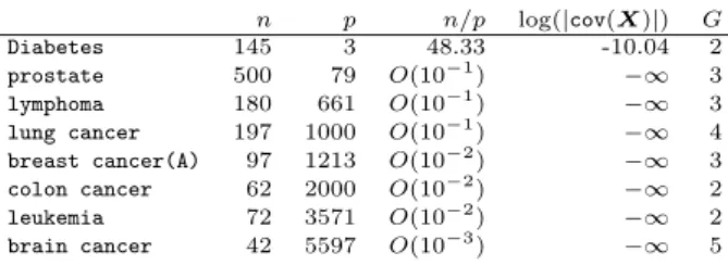
n p n/p log(|cov(X)|) G
Diabetes 145 3 48.33 -10.04 2
prostate 500 79 O(10−1) −∞ 3
lymphoma 180 661 O(10−1) −∞ 3
lung cancer 197 1000 O(10−1) −∞ 4
breast cancer(A) 97 1213 O(10−2) −∞ 3
colon cancer 62 2000 O(10−2) −∞ 2
leukemia 72 3571 O(10−2) −∞ 2
brain cancer 42 5597 O(10−3) −∞ 5
Table 1. The last column is the number of classes in the pattern
recognition task. The logarithm of the determinant of the covari-ance matrix is also provided to highlight just how ill conditioned the matrix is.
is organized as follows. In section two, we present ensemble learning for classifi-cation on contaminated high dimension low sample siz datasets with a special on random subspace learning via random forest, we provide a conceptual justification of the aspects responsible for the good predictive performance. In section three, we present a brief summary of discriminant analysis with an emphasis on where the need for robustification and regularization arises. We then discuss some of the most commonly used techniques of robustification, highlighting some of the limi-tations and merits of each method. In section four, we present the computational comparison of the techniques on real life data. In section five, we present a large simulation study, featuring various choices of the sample size n, dimensionality p, number of classes G, contamination rate ϵ and contamination size γ and correlation among the predictive variables ρ. We also highlight how various scenarios of these choices impact the average prediction error over R replications. In the section six, we present our conclusion and discussion along with a brief introduction to our future work dedicated to the regularized version of robust discriminant analysis in the HDLSS context.
2. Ensemble Learning Approach to Robust Classification It is often common in massive data that selecting a single model does not lead the optimal prediction. For instance, in the presence of multicollinearity which is almost inevitable when p is very large, function estimators are typically unstable, as they tend to exhibit rather large estimation variances. This issue of inflated variances gets even more amplified in the presence of data contamination. It makes sense that when data contains outliers, they will cause the variance of estimators to increase even more. Fortunately, ensemble learning can be used to create aggregate learning machines that substantially improve predictive performances. Recall that we have class labels y coming fromY = {1, 2, · · · , G} and predictor variables x =
(x1, x2,· · · , xp)⊤coming from a p-dimensional spaceX . Let bg(b)(·) be the bth
boot-strap replication of the estimated base classifierbg(·), such that (by)(b)=bg(b)(x) is the
bth bootstrap estimated class of x. The estimated response by bagging is obtained
using the majority vote rule, which means the most frequent label throughout the B bootstrap replications. Namely, bf(bagged)(x) = Most frequent label in bC(B)(x), where bC(B)(x) =
{
bg(1)(x),bg(2)(x),· · · , bg(B)(x) }
estimated label of x as b
f(bagged)(x) = arg max y∈Y { freqbC(B)(x)(y) } = arg max y∈Y { B ∑ b=1 ( 1{y=bg(b)(x)} )} .
In fact, when observation bagging (bootstrapping) is combined with attribute-bagging, we get the so-called random subspace learning of which random forest is a special case when base learners are trees. If T denotes the tree represented by the partitioning ofX into q regions R1, R2,· · · , Rq such thatX = ∪qℓ=1Rℓ, then,
all the observations in a given terminal node (region) will be assigned the same label, namely cℓ= argmax j∈{1,··· ,G} { 1 |Rℓ| ∑ xi∈Rℓ I(Yi= j) }
As a result, for a new point x, its predicted class is given by ˆ YTree=bgTree(x) = q ∑ ℓ=1 cℓIℓ(x),
where Iℓ(·) is the indicator function of Rℓ, i.e. Iℓ(x) = 1 if x∈ Rℓ andIℓ(x) = 0
if x /∈ Rℓ. While trees are known to be notoriously unstable because of their large
estimation variance, the random subspace learning approach via random forest does produce substantial predictive improvements, and we conjecture that the predictive improvements are due to the fact that by combining both bootstrapping on the observations with the selection of only a few dimensions out of the large number of dimensions, the influence of outliers is substantially reduced. In a sense, random subspace learning does induce robustness even if only implicitly.
Conjecture 1. LetD be the dataset under consideration. Assume that a proportion
ε of the observations inD are outliers. If ε < e−1, then the majority of the base
learning trees contributing to the random forest ensemble classifier will have a high probability of being robust in the sense that they will be constructed with a very low proportion of outliers.
Proof. The key idea of our conjecture rests on the fact that the combination of
bootstrapping and subspace selection leads to isolation of outliers, and thereby the robustness of most of the base learners used in the ensemble, and crucially, the use of voting further gives greater weight to that majority of outlier-free base learners, leading to the observed improvement in predictive performance. The following helps gain deeper insights in the outlier isolation capability of random subspace learning. Let xi ∈ D be a random observation in the original dataset D. Let D(b)denote the bth bootstrapped sample from D. Let Pr[x
i ∈ D(b)] represent the
proportion of observations that are in D but also present in D(b). It is easy to prove Pr[xi ∈ D(b)] = 1−
(
1−n1)n. In other words, if Pr[xi ∈ D/ (b)] = Pr[On]
denotes the observations fromD not present in D(b), we must have Pr[x
i∈ D/ (b)] =
(
1−n1)n = Pr[On]. Since Pr[On] is known to converge to e−1as n goes to infinity.
Therefore for each given bootstrapped sampleD(b), there is a probability close to
e−1 that any given outlier will not corrupt the estimation of location vector and scatter matrix parameters. Since the outliers as well as all other observations have an asymptotic probability of e−1 of not affecting the bootstrapped estimator that we build. Therefore over a large enough re-sampling process (large B), there will
be many bootstrapped samplesD(b)with very few outliers leading to a sequence of small covariance determinants as desired, if ε < e−1. It is therefore reasonable to deduce that by averaging this exclusion of outliers over many replications, robust estimators will naturally be generated by the RSSL algorithm
3. Covariance-based Classification Techniques
As emphasized from the beginning of this paper, we seek to demonstrate via compu-tational simulations and applications to real life data, that random forest, although not explicitly designed with robustness as its goal, proves to predictively outperform robustness-seeking algorithms. In this paper, all the alternatives to random forest are covariance-based methods, and in this section we present the most commonly used ones. Discriminant analysis is arguably one of the oldest and most commonly used approaches to pattern recognition. Under the assumption of an underlying Gaussian distribution for the class conditional densities, the main ingredient in linear discriminant analysis is the estimator [δk(x) given by
[ δk(x) =− 1 2(x− bµk) ⊤bΣ−1(x− bµ k) + logbπk, (3.1)
where bπk is the estimator of the prior class membership probability and bµ is the
empirical (sample) mean in class k, while bΣ is the estimator of the covariance matrix common to all the classes. It turns out that both the estimated locationbµk and the estimated scatter matrix bΣ are sensitive to outliers, making the estimated discriminant function non robust under contamination. In the context of prediction, non-robustness leads to poor predictive performances due the fact the presence of outliers in the explanatory variables causes the vital components of the discriminant function to be biased. We therefore need robust methods to estimate both location and scatter parameters in order to decrease the prediction error. When in addition we have p much larger than n, we encounter the extra problem of non-invertibility of bΣ. Typically, one can solve this problem by selecting few subset of variables. However, a more general approach deals with the problem by regularizing bΣ using eΣ = bΣ + λIp with λ∈ (0, ∞), or a convex and more general version of it where
eΣ = (1 − α)bΣ +α
ptrace( bΣ)Ip (3.2)
with α ∈ (0, 1). Some of the earliest work on regularized discriminant analysis include the seminar paper by [12], and later applications by [14], just to name a few. Many authors have contributed extensively in the area of regularized discriminant analysis. Clearly, in the presence of both outliers and high dimensionality, one needs to both robustify and then regularize. In the subsequent section, we mainly focus on the kind of robustification that deals with contaminated high dimensionality through a suitable combination robust PCA and projection pursuit [24], [38]. 3.1. Robust Estimation Methods for Linear Discriminant Analysis. In section two, one the challenges of discriminant analysis came from the fact that in the presence of outliers, the location and scatter estimates are not reliable because they are not robust. Many authors have contributed a wide variety of approaches all aimed at at robustifying LDA. One of the earliest approaches used to address this problem is a technique known as Minimum Covariance Determinant (MCD) introduced and de-veloped by [30], [32]. The literature on robust discriminant analysis has blossomed
recently, with many papers studying and exploring various extensions of MCD. In this paper, we will be comparing the predictive performances of extensions devel-oped by ([5]), then the one explored by [17] and [21]. We will also look into the predictive performances of MCD extensions proposed by ([21]), and the ones de-veloped by [37], [16]. Another paper extending the work on MCD is contributed by [19]. It is important to note that all the above mentioned variations on the MCD theme have been implemented in R with packages like rrcov and rrcovHD readily available for immediate installation and use. Our goal in this paper is to consider different scenarios of contamination in high dimensional spaces, and then compare the performances of existing techniques, with the finality of establishing the conditions under which each one of the techniques performs best. [30]’s original MCD estimator is quite intuitive and can be briefly described as follows: given n observations x1, x2,· · · , xn taken from a p-dimensional spaceX ⊂ Rp, with true
location vector µ and true scatter matrix Σ, find the subset of h observations out of n such that the corresponding sample (estimated) covariance matrix yields the smallest determinant. In other words, we must have
det( bΣ(γ(MCD))) = min
γ∈{0,1}n
{
det( bΣ(γ)) } where γ∈ {0, 1}n simply represents the indicator vector such that γ
i = 1 if
obser-vation i is among the h chosen, and γi= 0 if it is not. Obviously, the final indicator
vector γ(MCD)chosen by the MCD method is such that length(γ(MCD)) =|γ(MCD)| = h. Also, we use the notation bθ(γ) to denote the estimator of θ based on only the
ob-servations selected by the indicator vector γ. Essentially, the MCD estimator of the location parameter µ is defined by the mean of that subset γ(MCD)and the MCD estimator of the scatter matrix parameter Σ is defined by the covariance of that subset γ(MCD). More specifically,
bµMCD=bµ(γ
(MCD)) and Σb
MCD= bΣ(γ(MCD)).
In practice, bΣMCD is chosen in such a way that it is a multiple of its covariance matrix. The multiplicative factor is chosen in such a way that bΣMCD is consistent at the multivariate normal model and unbiased for small samples ([26]). The MCD algorithm can be formulated as an optimization problem
( bH,bµH, bΣH) = argmin µ,Σ,H {E(µ, Σ, H)} where E(µ, Σ, H) = log{det(Σ)} + 1 h ∑ i∈H (xi− µ)⊤Σ−1(xi− µ).
The MCD approach can be summarized in pseudo-code format as follows: Algorithm 1 Minimum Covariance Determinant (MCD)
1: Select h observations, and form the datasetDH. H ⊂ {1, · · · , n}.
2: Compute the empirical covariance bΣH and mean bµH.
3: Compute the Mahalanobis distances d2 b
µH, bΣH
(xi), i = 1,· · · , n
4: Select the h observations having the smallest Mahalanobis distance.
The seminal MCD algorithm proposed by [30] turned out to be rather slow and did not scale well as a function of the sample size n. That limitation of MCD led its author to creation of the so-called FAST-MCD [33]. Now, the MCD approach requires that n
2 ≤ h < n, with h = [(n + p + 1)/2] yielding the maximal breakdown
point. Central to MCD is the fact that h must be determined or set. In fact, it should be noted that the MCD estimator cannot be computed when p > h, since
such a scenario would mean having a singular covariance matrix for any h−subset.
It turns out that the whole MCD machinery needs n≥ 2p in order to function at
all. For our high dimension low sample size problems for which p≫ n, it is
obvi-ous that the basic formulation of MCD does not work. We discuss a little later the
extension of MCD known as regularized MCD whereby the estimates of interest are obtained in their regularized version. Even within the satisfaction of the n > 2p requirement, MCD is essentially very computationally intensive for the simple rea-son that the need to select a subset combinatorially to optimize a criterion requires a number of computing operations that can explode for even small sample sizes. Many faster versions of the basic MCD algorithm have been suggested, led by [31]. As we shall see later in our computations, different variants of MCD lead to some-times drastically different predictive performances. In the context of discriminant analysis, one of the obvious limitations of MCD lies in the fact that it trims all the classes/groups equally. Such an equal treatment of all the groups is potentially inefficient in the presence of uncontaminated groups. Many other drawbacks of the basic MCD approach to discriminant analysis have been scrutinized and addressed by authors such as [17], [21], [3], [5]. Each of these variants was proposed in order to address/solve a perceived limitation/drawback of the basic MCD approach. Un-fortunately, in turns out all these variants of MCD only work when p is less than n. In fact most of them require n to be at least greater than 2p. In order to deal with n less than p situations one had to abandon MCD in its present form. As a matter of fact, we are currently working on an extension of the MCD approach that combines robustification and regularization to address HDLSS situation with n/p arbitrarily very small. In this paper however, we explore two non-MCD based techniques, namely robust SIMCA (described later) and projection pursuit (PP) discriminant analysis. As we will see in the computational section, PP will proved to be quite flexible but unfortunately fail when n/p gets to small (less than to 10−2). We will see later that PP yields relatively poor predictive performances when the number of classes is greater than 2 and/or the intrinsic dimensionality of the input space is inherently high.
3.2. SIMCA approach to High Dimensional Robust Classification. Soft Independent Modelling of Class Analogies (SIMCA) was introduced by [39]. [2] ex-plain that SIMCA ability to classify high dimensional data comes from the fact that it is based on a clever adaptation of principal component analysis (PCA). Thanks to the supervised nature of discriminant analysis (class membership known), SIMCA proceeds by performing principal component analysis in each of the G classes sep-arately. Essentially, SIMCA can be summarized as an approach that combines robust PCA within each group based on robust covariance estimation to achieve good predictive performances in classification. More details on SIMCA can be found in [21], [20] [2] and [38]. SIMCA has been widely applied to areas as diverse as image analysis, microarray gene expression classification, and many other fields
where data exists with n much less than p. An implementation of Robust SIMCA is provided through the R package rrcovHD, and will be used in our comparison of predictive performances of high dimensional robust classifiers.
3.3. Projection Pursuit Approach for Robust Linear Discriminant Anal-ysis. From the seminal article [11], many authors like [10], [9] have developed applications and extensions of PP to wide variety of statistical problems. There have also been many theoretical justifications and discussions of the strengths and appeal of PP [18], [15]. PP has also been used in discriminant analysis and outlier detection[23] and [27]. [24] presents one of the most recent developments on PP for robust discriminant analysis in high dimensional spaces. Her work builds first on the original PP idea as presented and developed by [11] and [18], and combines robustness strategies and the foundational idea of PP presented in the above defini-tion, to achieve robust linear discriminant analysis in high dimensional spaces. Four of the seven techniques compared in this paper are based on the PP approach to robustness linear discriminant analysis in high dimension spaces. As we’ll see later though, it will turn out that PP techniques will fail - somewhat catastrophically at times - when the intrinsic dimensionality of the data is high. This is unsurprising, since the very idea of PP presupposes the existence of a lower dimensional space as the true/intrinsic basis of the data.
4. Computational Comparison of Predictive Performances We now consider comparing the predictive performances of the techniques described earlier on real life data. Among other things, we present the apparent (training) error and the true (test) error which in this case is more precisely average test error over R replications as defined in (1.1).
AVTE( bf ) = 1 R R ∑ r=1 { 1 m m ∑ i=1 ℓ(y(r)i , bfr(x (r) i )) } .
Throughout this paper, each replication randomly assigns 2/3 of the data to the training set and 1/3 to the test set. We do not consider a validation set because none of the techniques is based on a tuning parameter. We use R = 200 replications. We analyze 7 different datasets, six of which are high dimension low sample size (HDLSS) microarray gene expression datasets. For clarity and completeness, we present both the tables and the plots depicting the predictive performances of the methods explored and analyzed.
4.1. Description of the datasets. (i) Diabetes data: Our first data set deals with diabetes. It contains 145 observations, 3 variables and three classes. This is obviously not a high dimensional dataset, but we use it here to reveal the stark differences in performance between methods when one switches from large n small
p to large p small n. This dataset is available in the R package called mclust
contributed by [29]. (ii) Ceramic pottery data: This pottery data set was analysed by [35]. Other authors have used it to test the robustness of their methods, namely [4] and later [24]. Please note that these first two datasets are qualitatively different from all the other datasets explored in this paper. Indeed, all the other 5 remaining datasets we explore here have in common the fact that they are all microarray gene expression data sets. (iii) Prostate cancer data: This data
set comes from microarray gene expression profiles/levels on prostate cancer, and is a subset of a much larger data set from a study by [34]. This dataset has 37 samples classified as recurrent and 42 as non-recurrent primary prostate tumor.
(iv) Lymphoma data: The following data set deals with Lymphoma and contains
180 observations and 661 variables. (v) Lung cancer data: This dataset on lung cancer s just one of many existing lung cancer datasets. The version we explore in this paper contains 197 observations and 1000 variables. (vi) Colon cancer data: From [1], it contains 62 observations on subjects classified into two groups (G1: subjects with colon cancer, with 40 observations; G2: healthy subjects, with 22 observations) and measured on 2000 variables (gene expression levels). The aim is to predict, as accurately as possible, the disease status from the gene expression levels. This is a well known data set in the modern classification literature (e.g., References from the paper) and the original version is available in the colonCA R package from Bioconductor. The raw data is not normalized/preprocessed, which may lead to very bad classification results. Therefore a simple normalization procedure was applied: the data were log-transformed and after that each row was individually centered using its median. (vii) Leukemia data: In this Leukemia data set, there are 3571 variables(features), 72 samples ([13]). (viii) Brain cancer data: The last data set considered in this paper is a brain cancer dataset ([28]). The total number of patients in this case is n = 42, each represented by p = 5597 microarray gene expression features, covering 5 different types of brain cancer. Using the packages R packages rrcov and rrcovHD, we first computed the apparent error for each of the methods on all the datasets mentioned above.
4.2. Comparisons of Methods on Real Data Using the Apparent Error. Although the core of our work in this paper is focused on predictive performance as stated right from our introduction, we devote this subsection to comparisons based on the apparent (training) error, following from [37] and [24] who performed similar comparisons. At the very least, the computation (or attempt thereof) of the apparent misclassification rates gives a rough idea of how well the method might perform predictively, when they can be applied at all.
n
p 1453 = 48.33 50079 = 0.158 180661 = 0.272 1000197 = 0.197 200062 = 0.031 357172 = 0.020 559742 = 0.0075 Diabetes Prostate Lymphoma Lung Colon Leukemia Brain
Classic 13.10 NA NA NA NA NA NA
Linda 10.35 NA NA NA NA NA NA
PP 27.58 29.11 55.00 21.83 11.29 5.55 52.38
SIMCA 11.72 35.44 9.44 5.58 9.68 12.50 NA
Table 2. Apparent misclassification rates for the classical and robust estimators under different scenarios
As can be seen on Table (2), Linda (which is an R implementation of the MCD approach) and classic LDA only work when n/p is greater than 1, in this case on the diabetes data. PP and SIMCA do handle HDLSS (n/p < 1), with the exception
that SIMCA fails when n/p < 10−2. When they can both be applied, there is no
clear winner between PP and SIMCA: on some datasets, PP outperforms SIMCA, but on other datasets, it is the other way round. This seems to indicate that besides the impact of n/p, there is also the effect of the internal geometry of the data.
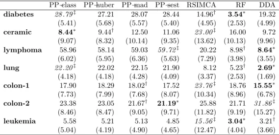
4.3. Comparisons of Methods on Real Data Using the Average Test Er-ror. In the interest of comparing the predictive optimality of the techniques ex-plored, we now present the performances of 4 different variants of PP discrimi-nation, against robust SIMCA, RF and Diagonal Discrimination Analysis (DDA). Here, we use R = 200 replications, and some of the results are summarized in Table (3) and Figure (1). As revealed in Table (3), one of the most immediate remark that emerges from our computations is the fact that SIMCA comes out as the worst in predictive performance 3 times, which is far more than any other method. SIMCA also never comes out as best. We actually provide greater details about this mediocre aspect of SIMCA in the simulated data section later. Another note-worthy aspect of these computations is the fact that DDA appears to perform very well, specifically emerging as the best 3 times (which is more times than any other technique). Given the fact DDA operates under the strong assumptions of uncor-relatedness of the predictor variables, we are let to infer that most of the datasets, especially those on which DDA has the best predictive performances, are inherently very high dimensional. In fact, this line of thought is somewhat supported by the fact overall, PP, which relies on the existence of a lower dimensional projection of the data, is the most unstable of the all the methods involved as shown clearly by Figure (1) where PP depicts huge spikes corresponding to large prediction errors. As depicted on the right panel of Figure (1), the lymphona data causes PP to fail miserably, probably because the intrinsic dimensionality of this data is so high that the projections fail to find lower dimensional representations. RF on the other hand provides what we perceive as the most stable of all the performances: it can be seen in Table (3) and Figure (1) that RF never comes last, and is usually best or second best, with no instability spikes. As a matter of fact, the right panel of Figure (1) shows the superior performance of RF and DDA, and relatively good performance of SIMCA on the lymphoma data, whereas all the PP variants fail catastrophically.
4.4. Comparison of Predictive Performances on Simulated Data. Based on the computations performed earlier on real life HDLSS microarray gene expression datasets, some patterns began to emerge, among which the overall stability and relatively strong predictive performance of RF, a method not structurally aimed at robustness. We also noticed that PP is a very unstable method, typically producing the worst performances on most data sets. Despite all these initial findings, we still do not have a general characterization of which aspects of the data drive the performances of each method. In this section, we use a thorough simulation study with various aspects of data characteristics, with the finality of determination what makes methods work well. For simplicity however, we use the first Σ with τ = 1 throughout this paper. For the remaining parameters, we use ϵ∈ {0, 0.05, 0.15},
κ∈ {9, 25, 100}, G ∈ {2, 3} and ρ ∈ {0, 0.25, 0.75} and p ∈ {10, 100, 1000}. As the
vector of ϵ values shows, we consider 3 different levels of contamination, namely no contamination, mild contamination and strong contamination.
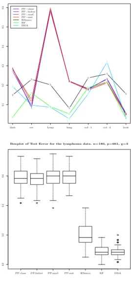
4.4.1. Uncontaminated Data. We first consider the performances of the techniques under an uncontaminated regime, i.e. ϵ = 0. Our first simulation on under this regime looks at combination where the number of classes is G = 2 and than in-vestigate the effect of ρ and p (input space dimension). As the plots all reveal, PP appears to perform very well (usually outperforming all the other methods)
PP-class PP-huber PP-mad PP-sest RSIMCA RF DDA diabetes 28 .79‡ 27.21 28.07 28.44 14.96† 3.54∗ 19.32 (5.41) (5.68) (5.57) (5.40) (4.95) (2.53) (4.99) ceramic 8.44∗ 9.44† 12.50 11.06 23 .00‡ 16.00 9.72 (9.07) (8.32) (10.14) (9.35) (13.62) (10.13) (9.96) lymphoma 58.96 58.14 59.03 59 .72‡ 20.22 8.98† 8.64∗ (6.02) (5.95) (6.36) (5.63) (7.29) (3.98) (3.55) lung 22 .20‡ 22.02 22.15 21.90 8.12 5.23† 2.69∗ (4.18) (4.18) (4.28) (4.09) (3.37) (2.53) (1.69) colon-1 17.90 18.29 18.02† 17.52 23 .76‡ 18.76 15.55∗ (7.73) (7.99) (7.68) (8.07) (10.34) (8.96) (6.78) colon-2 23.38 23.05 21.67† 21.19∗ 25.88 21.71 31 .86‡ (8.46) (8.47) (9.05) (9.71) (11.82) (9.19) (15.27) leukemia 5.58 5.21 5.13 4.85 15 .56‡ 3.04∗ 3.21† (5.04) (4.19) (4.90) (4.65) (12.47) (4.04) (3.66) Table 3. Average test error along with the corresponding
stan-dard deviation in parentheses. The star (*) is used to indicate the method with the best predictive performance, while the double dagger (‡) indicates the worst predictive performance. The dagger
(†) identifies the second best. The absence of prostate and brain is
due to the fact that many methods explored could not even handle them. SIMCA for instance could not handle the brain cancer data set.
whenever intrinsic dimensionality of the data is low (captured by ρ very high) and the number of classes is 2 (Binary classification task).
PP-class PP-huber PP-mad PP-sest RSimca RF DDA
10 58.26 59.22 61.19 61.26 41.11 45.11 43.26
100 54.11 50.89 53.33 55.63 40.44 42.00 43.44 1000 44.44 35.26 35.74 35.96 30.81 28.70 35.89 2000 44.17 34.00 34.28 34.67 30.89 32.44 38.50
Table 4. Average test error on the uncontaminated simulated data with g = 3 and ρ = 0.75. We herein reveal for each of the 7 methods, the effect of the input space dimension p on the average test error.
Table (4) clearly reveals that PP does not work well n multi-categorical classifica-tion. With the number of classes just equal to 3, PP yields the worst predictive performance, regardless of the value of the overall correlation among the variables. As we discuss much later, PP typically performs well in binary classification when
ρ is relatively large. But clearly, as depicted in Table (4), PP, at least in the
imple-mentation used here does NOT handle multiclass tasks well, even when the data is potentially representable in a lower dimensional space (large ρ). It is important to emphasize that this behavior of PP noticed here on uncontaminated data carries over to contaminated at various rates of contamination. Figure (2) clearly shows different scenarios of predictive performances under different data characteristics
1 1 1 1 1 1 1 2 2 2 2 2 2 2 3 3 3 3 3 3 3 4 4 4 4 4 4 4 5 5 5 5 5 5 5 6 6 6 6 6 6 6 7 7 7 7 7 7 7
diab cer lymp lung col−1 col−2 leuk
PP−class PP−huber PP−mad PP−sest RSimca RF DDA 0.1 0.2 0.3 0.4 0.5 0.6
PP.class PP.huber PP.mad PP.sest RSimca RF DDA
0.0
0.2
0.4
0.6
Boxplot of Test Error for the lymphoma data. n=180, p=661, g=3
Figure 1. (left) Average test error as a function of n/p. The data sets appear on the x axis in decreasing order of n/p. The first one(diabetes) has n/p = 145/3 and the last one (leukemia) has
n/p = 72/3571; (right) Average test error on the lymphoma data
set for which n/p = 180/661, and the number of classes is g = 3. These box plots compare the predictive performances of all the 7 methods considered.
when the data has no contamination. The left panel corresponds to the case when the number of classes is 3 and the correlation among variables is very high. In this case, RF and SIMCA emerge as the best whereas PP fails. In the center, we see another excellent performance of RF. wth DDA emerging as the best while PP fails, this time due to the fact that ρ = 0. The right panel highlight the ideal conditions for PP, namely binary classification along with large correlation.
1
1
1 1
Test Error(p) for uncontaminated n=54, rho=0.75, g=3
2 2 2 2 3 3 3 3 4 4 4 4 5 5 5 5 6 6 6 6 7 7 7 7 10 100 1000 2000 PP−class PP−huber PP−mad PP−sest RSimca RF DDA 0.30 0.35 0.40 0.45 0.50 0.55 0.60 1 1 1 1
Test Error(p) for uncontaminated n=54, rho=0, g=2
2 2 2 2 3 3 3 3 4 4 4 4 5 5 5 5 6 6 6 6 7 7 7 7 10 100 1000 2000 PP−class PP−huber PP−mad PP−sest RSimca RF DDA 0.0 0.1 0.2 0.3 0.4 1 1 1 1 Test Error(p) for uncontaminated n=54, rho=0.75, g=2
2 2 2 2 3 3 3 3 4 4 4 4 5 5 5 5 6 6 6 6 7 7 7 7 10 100 1000 2000 PP−class PP−huber PP−mad PP−sest RSimca RF DDA 0.0 0.1 0.2 0.3 0.4
Figure 2. (left) Average test error on the uncontaminated sim-ulated data with g = 3 and ρ = 0.75. We herein reveal for each of the 7 methods, the effect of the input space dimension p on the average test error. (center) Average test error on the uncontami-nated simulated data with g = 2 and ρ = 0. We herein reveal for each of the 7 methods, the effect of the input space dimension p on the average test error. (right) Average test error on the uncontam-inated simulated data with g = 2 and ρ = 0.75. We herein reveal for each of the 7 methods, the effect of the input space dimension
p on the average test error.
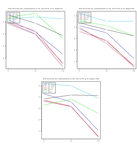
4.4.2. Effect of Mild Contamination. We now consider the performances of the techniques under a mildly contaminated regime, i.e. ϵ = 0.05. Our first simulation on under this regime looks at combination where the number of classes is g = 2 and than investigate the effect of ρ and p (input space dimension) and κ. Figure (3) reveals what we anticipated earlier, namely that PP performs well, typically emerging as the best predictive technique, when g=2 (binary classification) and ρ is large (intrinsically lower dimensionality of the data). In fact, under these two PP-favorable conditions, PP yields the best performance regardless of the size κ of contamination.
1 1
1 Test Error(p) for contaminated n=54, rho=0.75, g=2, kappa=9
2 2 2 3 3 3 4 4 4 5 5 5 6 6 6 7 7 7 10 100 1000 PP−class PP−huber PP−mad PP−sest RSimca RF DDA 0.1 0.2 0.3 0.4 1 1 1 Test Error(p) for contaminated n=54, rho=0.75, g=2, kappa=25
2 2 2 3 3 3 4 4 4 5 5 5 6 6 6 7 7 7 10 100 1000 PP−class PP−huber PP−mad PP−sest RSimca RF DDA 0.0 0.1 0.2 0.3 0.4 1 1 1 Test Error(p) for contaminated n=54, rho=0.75, g=2, kappa=100
2 2 2 3 3 3 4 4 4 5 5 5 6 6 6 7 7 7 10 100 1000 PP−class PP−huber PP−mad PP−sest RSimca RF DDA 0.1 0.2 0.3 0.4
Figure 3. Average test error on the mild contaminated simulated data with g = 2 and ρ = 0.75. We herein reveal for each of the 7 methods, the effect of the input space dimension p on the average test error.
Also noteworthy here is the fact that DDA fails for all the values of κ when ρ is large. Finally, we also notice that RF does reasonably well, while SIMCA gets progressively worse as κ increases.
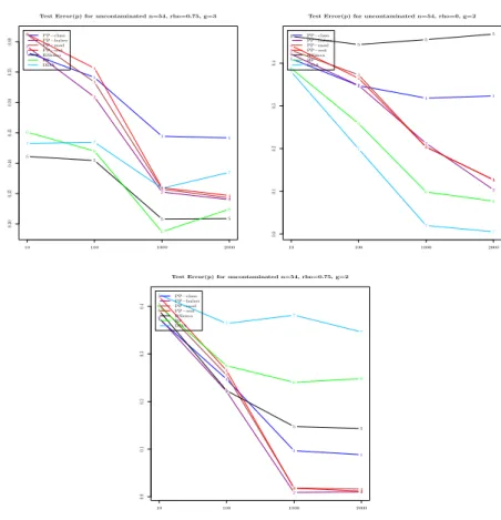
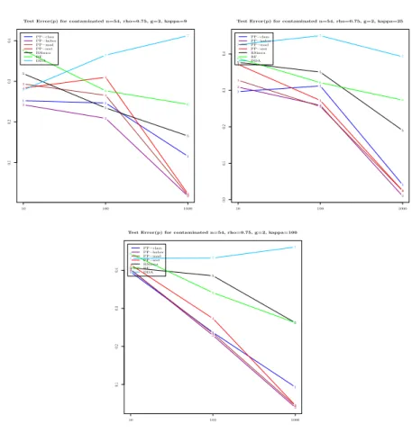
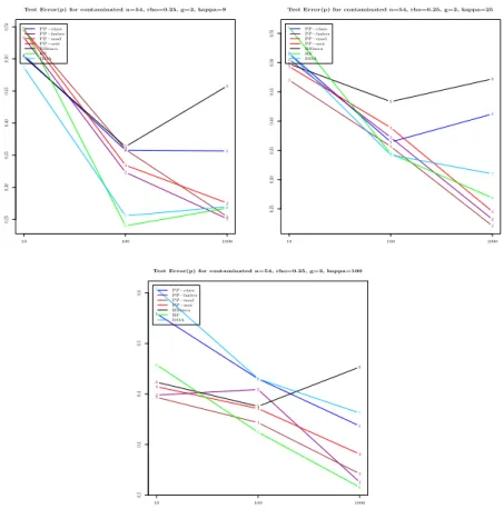
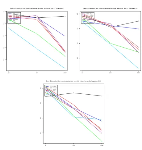
4.4.3. Effect of Strong Contamination. We now consider the performances of the techniques under a strongly contaminated regime, i.e. ϵ = 0.15. Our first simulation under this regime looks at combination where the number of classes is g = 2 and then investigates the effect of ρ and p (input space dimension) and κ.
We see in Figure (10) that under the strong contamination regime, RF emerges as the best in multi-categorical classification tasks, regardless of the correlation level and the size κ of contamination. SIMCA also performs very well under these conditions, typically taking the second place to RF in predictive performance. It can said that overall, RF and SIMCA are the most practical and applicable of all the techniques explored here, since they both do well for the realistic scenario of multicategorical classification with some rate of contamination.
1
1 1
Test Error(p) for contaminated n=54, rho=0.25, g=2, kappa=9
2 2 2 3 3 3 4 4 4 5 5 5 6 6 6 7 7 7 10 100 1000 PP−class PP−huber PP−mad PP−sest RSimca RF DDA 0.25 0.30 0.35 0.40 0.45 0.50 0.55 1 1 1 Test Error(p) for contaminated n=54, rho=0.25, g=2, kappa=25
2 2 2 3 3 3 4 4 4 5 5 5 6 6 6 7 7 7 10 100 1000 PP−class PP−huber PP−mad PP−sest RSimca RF DDA 0.25 0.30 0.35 0.40 0.45 0.50 0.55 1 1 1 Test Error(p) for contaminated n=54, rho=0.25, g=2, kappa=100
2 2 2 3 3 3 4 4 4 5 5 5 6 6 6 7 7 7 10 100 1000 PP−class PP−huber PP−mad PP−sest RSimca RF DDA 0.2 0.3 0.4 0.5 0.6
Figure 4. Average test error on the mild contaminated simulated data with g = 2 and ρ = 0.25. We herein reveal for each of the 7 methods, the effect of the input space dimension p on the average test error.
5. Conclusion and Discussion
We have presented a thorough comparison of the predictive performances of several robust classification methods on high dimension low sample size data. On both real life and simulated data, interesting patterns emerged. We noted for instance that the SIMCA method, by being somewhat very general tends to yield mediocre predictive performances when p is much larger than n, even though it rarely yield the worst among compared classification techniques. One of the most striking re-marks in our study has to do with projection pursuit, the clearest being the fact that projection pursuit seems to do well only in binary classification. As a matter of fact, for all the scenarios involving more than two classes, projection pursuit seems to fail miserably regardless of all the other aspects of the data. Strikingly also, when there are only two classes, projection pursuit yields the best predictive performance if the correlation among the input space variables is large. This leads us to conclude that projection pursuit as a method for robust discriminant analysis is - at least in its present form - only best suited to binary classification for data whose intrinsic dimensionality is very low. For us, the most striking observation
1
1
1 Test Error(p) for contaminated n=54, rho=0, g=2, kappa=9
2 2 2 3 3 3 4 4 4 5 5 5 6 6 6 7 7 7 10 100 1000 PP−class PP−huber PP−mad PP−sest RSimca RF DDA 0.1 0.2 0.3 0.4 0.5 1 1 1 Test Error(p) for contaminated n=54, rho=0, g=2, kappa=25
2 2 2 3 3 3 4 4 4 5 5 5 6 6 6 7 7 7 10 100 1000 PP−class PP−huber PP−mad PP−sest RSimca RF DDA 0.2 0.3 0.4 0.5 1 1 1 Test Error(p) for contaminated n=54, rho=0, g=2, kappa=100
2 2 2 3 3 3 4 4 4 5 5 5 6 6 6 7 7 7 10 100 1000 PP−class PP−huber PP−mad PP−sest RSimca RF DDA 0.2 0.3 0.4 0.5
Figure 5. Average test error on the mild contaminated simulated data with g = 2 and ρ = 0.0. We herein reveal for each of the 7 methods, the effect of the input space dimension p on the average test error.
lies with the performance of random forest. Indeed, as can be noted in all the computational results presented earlier, random forest tended to be the best over-all. More precisely, there was no instance where random forest yielded the worst performance, and in most cases, it was either the very best or the second best. As we explained earlier, this can be explained by the very mechanism of random forest in the sense that at every iteration of the construction of a random forest, not only is the estimator based on a subset of input variables, but also crucially the bootstrap mechanism leaves out a proportion e−1 of the sample. This left out fraction certainly contains some of the outliers. It is our conjecture as indicated earlier, that the fact of leaving out a fraction of the data allows random forest to weed out outliers or at least average out their effect. Hence the inherent ability of random forest to achieve robustness by random subsampling. One could conjecture that the overall superior performance of random forest can be attributed to the fact it does both variable selection (by random subspace learning) thereby inherently addressing the extremely high dimensionality of the data, and also reduction (or even elimination) of the effect of outliers by subsampling. There is a sense here of
1
1
1 Test Error(p) for contaminated n=54, rho=0, g=3, kappa=9
2 2 2 3 3 3 4 4 4 5 5 5 6 6 6 7 7 7 10 100 1000 PP−class PP−huber PP−mad PP−sest RSimca RF DDA 0.2 0.3 0.4 0.5 0.6 0.7 1 1 1
Test Error(p) for contaminated n=54, rho=0.25, g=3, kappa=25
2 2 2 3 3 3 4 4 4 5 5 5 6 6 6 7 7 7 10 100 1000 PP−class PP−huber PP−mad PP−sest RSimca RF DDA 0.3 0.4 0.5 0.6 1 1 1 Test Error(p) for contaminated n=54, rho=0.75, g=3, kappa=100
2 2 2 3 3 3 4 4 4 5 5 5 6 6 6 7 7 7 10 100 1000 PP−class PP−huber PP−mad PP−sest RSimca RF DDA 0.3 0.4 0.5 0.6
Figure 6. Average test error on the mild contaminated simulated data with g = 3. We herein reveal for each of the 7 methods, the effect of the input space dimension p on the average test error.
a connection - however loose - between the subset selection of minimum covariance determinant (MCD) - recall that MCD select h < n observations that yield the minimum covariance determinant - and the out-of-bag observations derived from the bootstrap in random forest. Therefore, we intend to investigate further the re-lationship between the fraction/proportion e−1of random forest and the number h of observations used the MCD. We are also currently exploration various strategies of regularized MCD as a way to achieve robust classification in settings where n is much less than p.
Acknowledgements
Ernest Fokou´e wishes to express his heartfelt gratitude and infinite thanks to Our Lady of Perpetual Help for Her ever-present support and guidance, especially for the uninterrupted flow of inspiration received through Her most powerful intercession.
References
[1] U. Alon, N. Barkai, D.A. Notterman, K. Gish, S. Ybarra, D. Mack, and A.J. Levine. Broad patterns of gene expression revealed by clustering analysis of tumor and normal colon tissue
1
1
1 Test Error(p) for contaminated n=54, rho=0.75, g=2, kappa=9
2 2 2 3 3 3 4 4 4 5 5 5 6 6 6 7 7 7 10 100 1000 PP−class PP−huber PP−mad PP−sest RSimca RF DDA 0.1 0.2 0.3 0.4 1 1 1 Test Error(p) for contaminated n=54, rho=0.75, g=2, kappa=25
2 2 2 3 3 3 4 4 4 5 5 5 6 6 6 7 7 7 10 100 1000 PP−class PP−huber PP−mad PP−sest RSimca RF DDA 0.1 0.2 0.3 0.4 0.5 1 1 1 Test Error(p) for contaminated n=54, rho=0.75, g=2, kappa=100
2 2 2 3 3 3 4 4 4 5 5 5 6 6 6 7 7 7 10 100 1000 PP−class PP−huber PP−mad PP−sest RSimca RF DDA 0.1 0.2 0.3 0.4 0.5
Figure 7. Average test error on the strongly contaminated sim-ulated data with g = 2 and ρ = 0.75. We herein reveal for each of the 7 methods, the effect of the input space dimension p on the average test error.
probed by oligonucleotide arrays. Proceedings of the National Academy of Sciences of the
United States of America,, 96(12):6745–6750, 1999.
[2] S. Bicciato, A. Luchini, and C. Di Bello. Pca disjoint models for multiclass cancer analysis using gene expression data. Bioinformatics,, 19(5):571–578, 2003.
[3] A. Christmann and R. Hable. On the bootstrap approach for support vector machines and related kernel based methods. In Proceedings 59th ISI World Statistics Congress,, Hong Kong, 25-30 August 2013. Session CPS018.
[4] R.A. Cooper and T.J. Weekes. Data, Models, and Statistical Analysis. Barnes and Noble,, New York, 1983.
[5] C. Croux and C. Dehon. Robust linear discriminant analysis using s-estimators. The Canadian
Journal of Statistics,, 29(2):473–493, 2001.
[6] P. Filzmoser, S. Serneels, R. Maronna, and P.J. Van Espen. Robust multivariate methods in chemometrics. In B. Walczak, R.T. Ferre, and S. Brown, editors, Comprehensive
Chemomet-rics,, pages 681–722. 2009.
[7] P. Filzmoser and V. Todorov. Review of robust multivariate statistical methods in high dimension. Analytica Chimica Acta,, 705(1-2):2–14, 2011.
[8] P. Filzmoser and V. Todorov. Robust tools for the imperfect world. Information Sciences,, 245:4–20, 2013.
1
1
1 Test Error(p) for contaminated n=54, rho=0.25, g=2, kappa=9
2 2 2 3 3 3 4 4 4 5 5 5 6 6 6 7 7 7 10 100 1000 PP−class PP−huber PP−mad PP−sest RSimca RF DDA 0.30 0.35 0.40 0.45 0.50 1 1 1 Test Error(p) for contaminated n=54, rho=0.25, g=2, kappa=25
2 2 2 3 3 3 4 4 4 5 5 5 6 6 6 7 7 7 10 100 1000 PP−class PP−huber PP−mad PP−sest RSimca RF DDA 0.20 0.25 0.30 0.35 0.40 0.45 1 1 1 Test Error(p) for contaminated n=54, rho=0.25, g=2, kappa=100
2 2 2 3 3 3 4 4 4 5 5 5 6 6 6 7 7 7 10 100 1000 PP−class PP−huber PP−mad PP−sest RSimca RF DDA 0.25 0.30 0.35 0.40 0.45 0.50 0.55
Figure 8. Average test error on the strongly contaminated sim-ulated data with g = 2 and ρ = 0.25. We herein reveal for each of the 7 methods, the effect of the input space dimension p on the average test error.
[9] J. H. Friedman. Exploratory Projection Pursuit. Journal of the American Statistical
Associ-ation, 82(397):249–266, 1987.
[10] J. H. Friedman and W. Stuetzle. Projection Pursuit Regression. Journal of the American
Statistical Association, 76(376):817–823, 1981.
[11] J. H. Friedman and J. W. Tukey. A Projection Pursuit algorithm for exploratory data analysis.
IEEE Trans. on computers, 23(9):881–890, 1974.
[12] J. H. Friedman and J.W. Tukey. A projection pursuit algorithm ror exploratory data analysis. In IEEE TRANSACTIONS ON COMPUTERS,. 1974.
[13] T.R. et. al. Golub. Molecular classification of cancer:discovery and class prediction by gene expression monitoring. Science,, 286:531537, 1999. doi: 10.1126/science.286.5439.531. [14] Y. Guo, T. Hastie, and R. Tibshirani. Regularized linear discriminant analysis and its
appli-cation in microarrays. Biostatistics, 8(1):86–100, 2006.
[15] P. Hall. On polynomial-based projection indices for exploratory projection pursuit. The
An-nals of Statistics, 17(2):589–605, 1990.
[16] D. M. Hawkins and G. J. McLachlan. High-breakdown linear discriminant analysis. Journal
of the American Statistical Association,, 92(437):136–143, 1997.
[17] X He and W.K. Fung. High breakdown estimation for multiple populations with applications to discriminant analysis. Journal of Multivariate Analysis,, 72(2):151–162, 2000.
1
1
1 Test Error(p) for contaminated n=54, rho=0, g=2, kappa=9
2 2 2 3 3 3 4 4 4 5 5 5 6 6 6 7 7 7 10 100 1000 PP−class PP−huber PP−mad PP−sest RSimca RF DDA 0.20 0.25 0.30 0.35 0.40 0.45 1 1 1 Test Error(p) for contaminated n=54, rho=0, g=2, kappa=25
2 2 2 3 3 3 4 4 4 5 5 5 6 6 6 7 7 7 10 100 1000 PP−class PP−huber PP−mad PP−sest RSimca RF DDA 0.2 0.3 0.4 0.5 1 1 1 Test Error(p) for contaminated n=54, rho=0, g=2, kappa=100
2 2 2 3 3 3 4 4 4 5 5 5 6 6 6 7 7 7 10 100 1000 PP−class PP−huber PP−mad PP−sest RSimca RF DDA 0.25 0.30 0.35 0.40 0.45 0.50
Figure 9. Average test error on the strongly contaminated sim-ulated data with g = 2 and ρ = 0.00. We herein reveal for each of the 7 methods, the effect of the input space dimension p on the average test error.
[19] M. Hubert and M. Debruyne. Minimum covariance determinant. WIREs Comp Stat, 2: 3643.
doi: 10.1002/wics.61, 2:3643, 2010.
[20] M. Hubert and S. Engelen. Robust pca and classification in biosciences. Bioinformatics,, 20(11):1728–1736, 2004.
[21] M. Hubert and K. Van Driessen. Fast and robust discriminant analysis. Computational
Sta-tistics and Data Analysis,, 45(2):301–320, 2004.
[22] Y. Kondo, M. Salibian-Barrera, and R. Zamar. A robust and sparse k-means clustering algo-rithm. arXiv preprint arXiv, (1201.6082), 2012.
[23] J-X. Pan, W-K. Fung, and K-T. Fang. Multiple outlier detection in multivariate data using projection pursuit techniques. Journal of Statistical Planning and Inference, 83(1):153–167, 2000.
[24] A. M. Pires. Projection-pursuit approach to robust linear discriminant analysis. Journal
Mul-tivariate Analysis,, (101):2464–2485, 2010.
[25] A.M. Pires. Robust linear discriminant analysis and the projection pursuit approach. In R. Dutter, P. Filzmoser, U. Gather, and P. J. Rousseeuw, editors, Developments in Robust
Statistics,, pages 317–329. Physica-Verlag HD, 2003. ISNB: 978-3-642-63241-9.
[26] G. Pison, S. Van Aelst, and G. Willems. Small sample corrections for lts and mcd. Metrika,, 55(1-2):111–123, 2002.
1
1
1 Test Error(p) for contaminated n=54, rho=0, g=3, kappa=9
2 2 2 3 3 3 4 4 4 5 5 5 6 6 6 7 7 7 10 100 1000 PP−class PP−huber PP−mad PP−sest RSimca RF DDA 0.3 0.4 0.5 0.6 1 1 1 Test Error(p) for contaminated n=54, rho=0.25, g=3, kappa=25
2 2 2 3 3 3 4 4 4 5 5 5 6 6 6 7 7 7 10 100 1000 PP−class PP−huber PP−mad PP−sest RSimca RF DDA 0.35 0.40 0.45 0.50 0.55 0.60 0.65 0.70 1 1 1 Test Error(p) for contaminated n=54, rho=0.75, g=3, kappa=100
2 2 2 3 3 3 4 4 4 5 5 5 6 6 6 7 7 7 10 100 1000 PP−class PP−huber PP−mad PP−sest RSimca RF DDA 0.4 0.5 0.6 0.7
Figure 10. Average test error on the strong contaminated simu-lated data with g = 3. We herein reveal for each of the 7 methods, the effect of the input space dimension p on the average test error.
[27] Jrg Polzehl and Deutsche Forschungsgemeinschaft. Projection pursuit discriminant analysis.
Computational Statistics and Data Analysis, 20:141–157, 1993.
[28] S. et al. Pomeroy. Prediction of central nervous system embryonal tumor outcome based on gene expression. Nature,, 415:436–442, 2002.
[29] G.M. Reaven and R.G. Miller. An attemp to define nature of chemical diabest using a mul-tidimensional analysis. Diabetologica,, 16:17–24, 1979.
[30] P. J. Rousseeuw. Least median of squares regression. Journal of the American Statistical
Association,, 79(388):871–880, 1984.
[31] Peter J. Rousseeuw and Katrien Van Driessen. A fast algorithm for the minimum covariance determinant estimator. Technometrics, 41:212–223, 1998.
[32] P.J. Rousseeuw. Multivariate estimation with high breakdown point. In W. Grossmann, G. Pflug, I. Vincze, and W. Wertz, editors, In Mathematical Statistics and Applications,, Dordrecht, 1985. Reidel Publishing Company.
[33] P.J. Rousseeuw and K. Van Driessen. A fast algorithm for the minimum covariance determi-nant estimator. Technometrics,, 41(3):212–223, 1999.
[34] A. Stephenson, A.J.and Smith, M.W. Kattan, J. Satagopan, V.E. Reuter, P.T. Scardino, and W.L. Gerald. Integration of gene expression profiling and clinical variables to predict prostate carcinoma recurrence after radical prostatectomy. Cancer,, 104(2):290–298, 2005.
[35] W.B. Stern and J.-P. Descoeudres. X-ray fluorescence analysis of archaic greek pottery.
[36] V. Todorov and P. Filzmoser. An object-oriented framework for robust multivariate analysis.
Journal of Statistical Software,, 32(3):1–47, 2009.
[37] V. Todorov and A. M. Pires. Comparative performance of several robust linear discriminant analysis methods. REVSTAT - Statistical Journal,, 5(1):63–83, 2007.
[38] K. Vanden Branden and M. Hubert. Robust classification in high dimensions based on the simca method. Chemometrics and Intelligent Laboratory Systems,, 79:10–21, 2005.
[39] S. Wold. Pattern recognition by means of disjoint principal components models. Pattern
Recognition,, 8(3):127–139, 1976.
Necla G¨und¨uz: Fen Fak¨ultesi, Istatistik B¨ol¨um¨u,Gazi ¨Universitesi, Ankara, Turkey
E-mail address: [email protected]
Ernest Fokou´e: School of Mathematical Sciences, Rochester Institute of Technology, Rochester, New York 14623, USA