IS S N 1 3 0 3 –5 9 9 1
NON-PROPORTIONAL HAZARDS WITH APPLICATION TO KIDNEY TRANSPLANT DATA
EMEL BA¸SAR
Abstract. The Cox proportional hazards (PH) model is the popular method for modelling censored survival data. The fundamental assumption of the Cox PH model is the proportionality of hazards in which the hazard ratio is linear in the covariates. However this assumption may not hold in some survival studies. Therefore, di¤erent non-parametric regression methods have been proposed to estimate the hazard ratio as a function of time when the proportionality of hazards can not be assumed. In this study a piecewise model and a non-parametric regression spline model have been considered for the non-proportional hazards. The models have been illustrated with kidney transplant data..
1. introduction
The Cox proportional hazards (PH) model introduced by Cox [4] has been widely used in analysis of survival data. The term proportional hazards refer to the fact that covariates have a multiplicative e¤ect on the hazards and the ratio of the haz-ards for di¤erent individuals is constant over the time. This assumption may not be met in all censored survival data set. The impact of a covariate on hazards may change during the follow-up. Several tests have been proposed to check the propor-tional hazards hypothesis [14]. However, after having rejected the PH hypothesis, it is not obvious how to summarize the e¤ect of a covariate [1].
The standard method for modelling the e¤ect of a predictor that violates the PH assumption is to include a time dependent covariate, representing an inter-action between the covariate and a parametric function of follow-up time and its shape represents the changes in hazard ratio during follow-up. Another method was proposed by Moreau et. al. [15]. They …tted a piecewise PH model. In that model, hazard ratio becomes a step function that is constant within each a priori deter-mined time interval but varies between intervals. However, the resulting estimates
Received by the editors March 12, 2007; Rev. June 1, 2007; Accepted: June 17, 2007. 2000 Mathematics Subject Classi…cation. Primary 62N01, 62G08; Secondary 62N02.
Key words and phrases. Cox regression, Proportional hazards, Regression splines, Survival analysis.
c 2 0 0 6 A n ka ra U n ive rsity
are unsmooth and impact of the number of intervals is not obvious. In the 1990’s several authors developed non-parametric methods for modeling time-dependent hazard ratio as a smooth ‡exible function of time [16].
Splines are a better tool for exploring nonlinear relationships and ‡exible statis-tical techniques. There are two classes of splines: regression splines and smoothing splines. Regression splines are piecewise polynomials joined at control points that are called knots. Linear splines constitute a set of connected line segments, which are continuous functions with discontinuous …rst derivative at the knots. Quadratic splines have continuous …rst derivatives, cubic splines continuous …rst and second derivatives. They are very attractive for non-parametric modeling; but, choosing the number of knots or the location of knots is arbitrary [19]. An alternative to the regression spline is the smoothing spline. The smoothing splines have knots located at every unique value of the continuous predictor variable, and include a penalty for over…tting. The smoothing splines have been used in generalized additive models [7].
A large number of works have been done on the regression spline methods and varying-coe¢ cient models. Some of these studies among the others are: Sleeper and Harrington [18], Gray [9], Hastie and Tibshirani [11], Gray [10], Hess [12], Kooperberg et al. [13], Rosenberg [17], Abrahamowicz et al. [1], Cai and Sun [3].
In this study, testing of PH hypothesis based on the Grambsch-Therneau test [8] has been considered. Time-dependent model, piecewise PH model with two and three intervals, and regression splines model with four degrees of freedom have been considered for modelling non-proportionality. These models are illustrated with the kidney transplantation data.
2. proportional hazards model
In the Cox PH model, introduced by Cox [4], the hazard at time t is de…ne as: (t; x) = 0(t) exp p X i=1 ixi ! (1) where, (t; x) is the hazard rate at time t for individual with covariate vector x. 1; 2; :::; p are the unknown regression parameters called log hazard ratios and represent the e¤ect of each covariate on the logarithm of the hazard. 0 is an unspeci…ed non-negative function of time called baseline hazard. The model assumes that the hazard ratio between two subjects with …xed covariates is constant. When the assumption of proportionality does not hold, the Cox PH model may produce biased results and the alternative models have to be considered.
3. piecewise proportional hazards model
The piecewise PH model incorporates non-proportional hazards in the Cox model by representing hazard ratio as a step function of time [15]. Hazard ratio is constant
within each of r pre-speci…ed time intervals but varies between the intervals. Within the i-th interval (j = 1; :::; r), the hazard is expressed by:
(t; x) = 0(t) exp p X i=1 ( i+ ji)xi ! (2) where 1i = 0. The log hazard ratio equals to i in the …rst interval and ( i+ ji) in the subsequent intervals for j = 2; :::; r. The PH model becomes a special case of the piecewise model [16]. In this study the piecewise analysis is limited with two and three intervals, because there are many failures on the beginning of the follow-up period.
4. regression splines model
A spline is a piecewise polynomial that has continuous derivatives at the points where pieces join. When a continuous covariate a¤ects the log hazard in a smooth fashion, a spline function is natural choice for approximating the covariate trans-formation [18].
The non-parametric spline model is de…ned as: (t; x) = 0(t) exp p X i=1 i(t)xi ! (3) where x = (x1; :::; xp) is a vector of p covariates, 0(t) is an unspeci…ed baseline hazard function corresponding to x = 0, and i(t) is the logarithm of the hazard ratio at time t corresponding to a unit increase in covariate xi. This model is gen-eralized PH model with the constant log hazard ratios i are replaced by estimable functions of time i(t). The e¤ects of some covariates may still be constant. It is assumed that non-constant functions i(t) lie in a pre-chosen polynomial regression spline space. Regression splines are smooth piecewise polynomials with pieces that join at knots. The degrees of polynomial pieces and the number and location of knots may vary. k is the spline order (or polynomial degree k 1) and m is the number of knots. A space of regression splines is linear, and its dimension is m + k. For each i the following expression can be written:
i(t) = ri
X j=1
ijgij(t) (4)
where ri is the dimension of regression spline space for i-th covariate and ij is the regression parameter and gij(t) are basis function for this space. A useful basis for this linear space is given by de Boor [5] and called B-splines. B-spline base functions are numerically well-conditioned. Model (3) can be rewritten as:
(t; x) = 0(t) exp 0 @ p X i=1 ri X j=1 ijyij(t) 1 A (5)
where yij(t) = gij(t)xi [1].
De Boor [5] gave an algorithm to compute B-splines of any degree from B-splines of lower degree. Because a zero-degree B-spline is a constant on one interval between two knots, it is simple to compute B-splines of any degree. The choice of knots has been a subject much research, too many knots lead to over…tting of the data, too few knots lead to under…tting [6].
The degree of freedom for the …t is given by the number of basis functions, equal to the number of …tted regression coe¢ cients. For regression splines, the degree of freedom equals the number of knots plus 1. One degree of freedom corresponds a straight line. Increasing the degrees of freedom corresponds to more complicated curves [19].
5. application to kidney transplant patients
The data has been collected from register of patients at Ba¸skent University Hospital and it consists of survival data of 93 patients who were operated kidney transplantation [2]. The beginning of the lifetimes is de…ned as the operation time and the end point of the lifetimes are the rejection of kidney or the death of the patients. The follow-up time is 35 months and the eighteen failures have been observed during the study period. Various covariates have been collected and only four of them included in this study. These covariates are patient age, donor age, disease duration and sex.
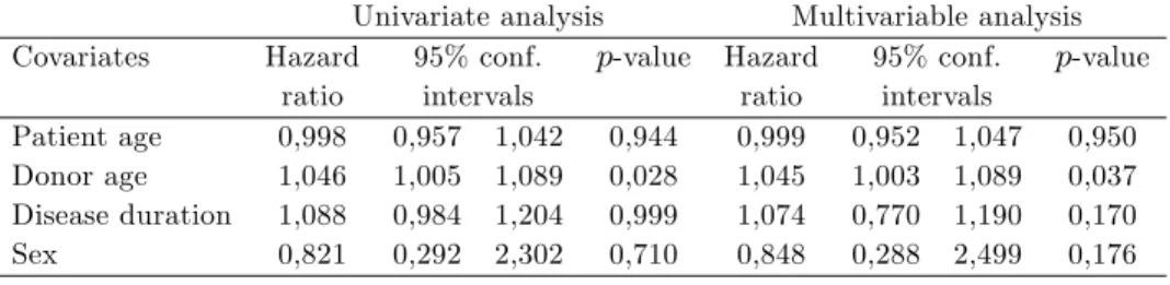
First, the Cox PH model is …tted to the data. The results of the univariate and multivariable Cox PH models are summarized in Table 1, giving the estimators of hazard ratios for each covariate and their con…dence intervals and its p-value from the likelihood ratio test. Donor age is the only covariate that shows a statistically signi…cant impact on the survival at the level of = 0:05 in the context of both the univariate and multivariable Cox PH models.
Table 1-Univariate and multivariable Cox proportional hazards analysis
Univariate analysis Multivariable analysis
Covariates Hazard 95% conf. p-value Hazard 95% conf. p-value
ratio intervals ratio intervals
Patient age 0,998 0,957 1,042 0,944 0,999 0,952 1,047 0,950
Donor age 1,046 1,005 1,089 0,028 1,045 1,003 1,089 0,037
Disease duration 1,088 0,984 1,204 0,999 1,074 0,770 1,190 0,170
Sex 0,821 0,292 2,302 0,710 0,848 0,288 2,499 0,176
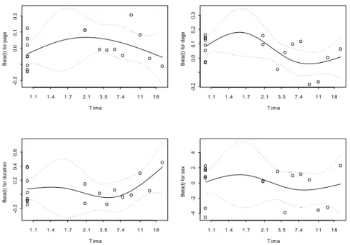
The proportional hazards model hypotheses are tested for each covariate based on scaled Schonfeld residuals [19]. In Figure 1 the plot of scale residuals are given against ordered time along with spline smooth together 90% con…dence intervals. The Grambsch-Therneau test has p-value= 0:041 for donor age and this provides the evidence that the covariate donor age violates the PH assumption at the level
of = 0:05. The impact of the donor age score clearly changes with time and this varying e¤ect can be seen in Figure 1. The other covariates do not show a time-varying pattern. The p-values for covariates patient age, disease duration, and sex are respectively 0:478, 0:584, and 0:567. When the assumption of proportionality does not hold, alternative models have to be considered.
For categorical covariates apparent non-proportionality can be handled by strati-…cation, but this is impossible for continuous covariates. To model non-proportional hazards, an interaction term between the covariates and a pre-speci…ed parametric function is included in the Cox PH model [4]. Several functions are considered in this study. These are f (t) = t, f (t) = ln t and f (t) =pt.
Table 2 demonstrates that some conclusions depend on the number of inter-vals, considered function and regression splines model. For patient age and disease duration, non-proportionality of hazards is signi…cant with two and three inter-vals. First two time-dependent models suggested that PH hypothesis is rejected for patient age, donor age and disease duration. For splines model, PH assumption is statistically signi…cant for all the covariates. In the piecewise model with two intervals and splines model p-value could not compute for sex.
T im e B et a( t) f or p age 1.1 1.4 1.7 2.1 3.5 7.4 11 18 -0 .2 0.0 0.1 0.2 T im e B et a( t) f or d age 1.1 1.4 1.7 2.1 3.5 7.4 11 18 -0 .2 0.0 0.1 0.2 0.3 T im e Beta(t) f or duration 1.1 1.4 1.7 2.1 3.5 7.4 11 18 -0 .2 0.2 0.4 0.6 T im e Be ta(t) fo r sex 1.1 1.4 1.7 2.1 3.5 7.4 11 18 -4 -2 0 2 4
Table 2- Testing the proportional hazards hypothesis p-values based on multivariable model
Piecewise model Time-dependent model Splines
Covariate Two intervals Three intervals t ln t pt
Patient age 0,004 0,015 0,002 0,000 0,006 0,707
Donor age 0,194 0,226 0,036 0,001 0,020 0,297
Disease duration 0,002 0,001 0,022 0,033 0,167 0,624
Sex - 0,216 0,375 0,022 0,234
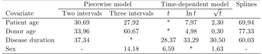
-Comparisons of goodness-of-…t of di¤erent univariate models by using the Akaike Information Criterion (AIC) are given in the Table 3. Lower AIC values indicate better …t. For each covariate, the best …tting model is identi…ed by ’ * ’. The numbers in the same row show the di¤erence in AIC values between respective models and the best model. AIC values in Table 3 show that time-dependent models …t much better than the other models.
Table 3- Goodness-of-…t of univariate models with di¤erences in AIC values
Piecewise model Time-dependent model Splines
Covariate Two intervals Three intervals t ln t pt
Patient age 30,69 27,92 * 7,97 2,30 69,94
Donor age 33,96 60,67 * 4,98 0,30 77,33
Disease duration 37,34 * 28,37 33,29 30,50 60,03
Sex - 14,18 6,59 * 1,63
-Table 4 shows the results of testing of the proportionality for multivariable mod-elling. In the multivariable analysis three homogeneous versions of time-dependent models were speci…ed as a priori. Each of these models represented time-dependent e¤ects of all covariates by one of the three functions that are f (t) = t, f (t) = ln t, f (t) = pt. The optimal model is de…ned as a posteriori and the e¤ect of each factor was represented by the function that …tted best in the univariate analysis. The …rst row of Table 4 shows AIC values, as expected, the optimal model …ts the data better than the three other time-dependent models. The spline model has the biggest AIC value.
Table 4- Testing the proportional hazards model hypothesis for multivariable models t ln t pt Optimal Splines AIC 78,1 86,9 80,3 77,8 164,7 Overall test of PH 86,0 77,1 83,7 86,2 7,30 p-value <0,00 <0,00 <0,00 <0,00 0,504
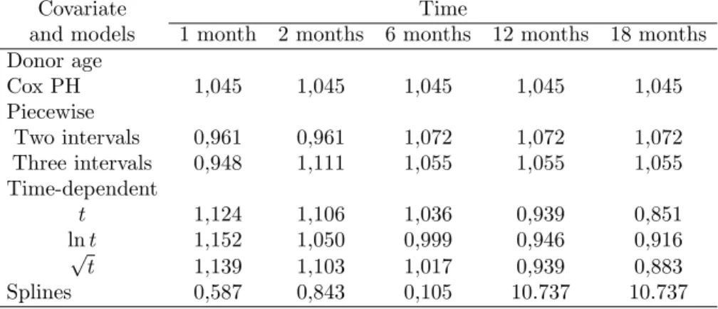
Table 5 represents the hazard ratio estimates for donor age with di¤erent models. The proportional hazards assumption fails to hold only the donor age. Because of this reason, in these models four covariates are included and only the hazard ratio of donor age has time-dependent e¤ect. All models are statistically signi…cant and the hazard ratios are decreased over time except the splines model.
Table 5- Hazard ratio estimates for donor age
Covariate Time
and models 1 month 2 months 6 months 12 months 18 months Donor age Cox PH 1,045 1,045 1,045 1,045 1,045 Piecewise Two intervals 0,961 0,961 1,072 1,072 1,072 Three intervals 0,948 1,111 1,055 1,055 1,055 Time-dependent t 1,124 1,106 1,036 0,939 0,851 ln t 1,152 1,050 0,999 0,946 0,916 p t 1,139 1,103 1,017 0,939 0,883 Splines 0,587 0,843 0,105 10.737 10.737 6. discussions
In this study a kidney transplantation data is used to assess the performance of di¤erent models in univariate and multivariable analysis. The piecewise PH models, Cox PH model with time-dependent covariates and splines model are con-sidered for this purpose. The results of piecewise models depend on the arbitrary number of time intervals and are di¢ cult to implement in multivariable modelling as mentioned in [16]. In the Cox model with time-dependent covariates the selec-tion of parametric funcselec-tion is very important. Restricting the analysis to a single a priori selected parametric function may result biased estimates. The optimal model is de…ned by estimating di¤erent parametric function and selecting the best …tting model. The di¤erent parametric estimates …t data equally well and also induces overestimation bias. The regression spline model is ‡exible modelling for non-proportionality of the hazard ratio. But surprisingly, spline model did not …t the data well. Probably that is because the data is collected in relatively short-term study and most of the failures are observed at the beginning of the study.
ÖZET
Cox orant¬l¬ hazard (OH) modeli durdurulmu¸s ya¸sam sürdürme verisini modellemek üzere en çok kullan¬lan yöntemdir. Cox OH modelinin temel varsay¬m¬ hazard¬n orant¬l¬ olmas¬d¬r. Hazard oran¬ise e¸sde¼gi¸skenler üzerinde do¼grusald¬r. Baz¬ya¸sam sürdürme çal¬¸smalar¬nda bu varsay¬m sa¼glanamayabilir. Hazard¬n orant¬l¬ olmas¬n¬n varsay¬lamad¬¼g¬ durumda, hazard oran¬n¬ zaman¬n bir fonksiyonu olarak tahmin etmek üzere farkl¬ parametrik olmayan regresyon yöntemleri önerilmi¸stir.
Bu çal¬¸smada orant¬l¬ olmayan hazard için, parçal¬ orant¬l¬ ha-zard modeli ve parametrik olmayan regresyon spline modeli dikkate al¬nm¬¸s ve modeller böbrek nakli verisine uygulanm¬¸st¬r.
References
[1] Abrahamowicz, M., MacKenzie, T., Esdaile, J. M., Time-dependent hazard ratio: modelling and hypothesis testing with application in lupus nephritis, Journal of the American Statistical Association, 91(1996), 1432-1439.
[2] Ba¸sar, E., Applications of some statistical technique used in life table analysis to the kidney transplantation data, Unpublished Ph. D., thesis, Science Institute of Hacettepe University. 1993.
[3] Cai, Z., Sun, Y., Local linear estimation for time-dependent coe¢ cients in Cox’s regression models, Scandinavian Journal of Statistics, 30(2003), 93-111.
[4] Cox, D. R. Regression models and life tables, Journal of the Royal Statistical Society, Ser. B, 34(1972), 187-220.
[5] De Boor, C., A Practical Guide to Splines, Springer, New York, 1978.
[6] Eilers, P. H. C., Marx, B. D., Flexible smoothing with B-splines and penalties, Statistical Science, 89(1996), 89-121.
[7] Eisen, A. E., Agalliu, I., Thurston, S. W., Coull, B. A., Checkoway, H., Smoothing in occu-pational cohort studies: an illustration based on penalised splines, Occuoccu-pational and Envi-ronmental Medicine, 61(2004), 854-860.
[8] Grambsch, P. M., Therneau T. M., Proportional hazards test and diagnostics based on weight residuals, Biometrika, 81(1994), 515-526.
[9] Gray, R. J., Flexible methods for analyzing survival data using splines, with applications to breast cancer prognosis, Journal of the American Statistical Association, 87(1992), 942-951. [10] Gray, R. J., Spline-based test in survival analysis, Biometrcs, 50(1994), 640-652.
[11] Hastie, T., Tibshirani, R., Varying-coe¢ cient models, Journal of the Royal Statistical Society, Ser. B, 55(1993), 757-796.
[12] Hess, K. R., Assessing time-by-covariate interactions in proportional hazards regression mod-els using cubic spline functions, Statistics in Medicine, 13(1994), 1045-1062.
[13] Kooperberg, C., Stone, C. J., Truong, Y. K., Hazards regression, Journal of the American Statistical Association, 90(1995), 78-94.
[14] Lin, D. Y., Wei, L. J., Goodness-of-…t test for the general Cox regression model, Statistica Sinica, 1(1991), 1-17.
[15] Moreau, T., O’Quigley, J., Mesbah, M. A., A global goodness-of-…t statistic for the propor-tional hazards model, Applied Statistics, 34(1985), 212-218.
[16] Quantin, C., Abrahamowicz, M., Moreau, T., Bartlett, G., MacKenzie, T., Tazi, M. A., Lalonde, L., Faivre, J., Variation over time of the e¤ects of prognostic factors in a population-based study of colon cancer: comparison of statistical models, American Journal of Epidemi-ology, 150(1999), 1188-1200.
[17] Rosenberg, P. S., Hazard function estimation using B-splines, Biometrics, 51(1995), 874-887. [18] Sleeper, A. L., Harrington, D. P., Regression splines in the Cox model with application to covariate e¤ects in liver disease, Journal of the American Statistical Association, 85(1990), 941-949.
[19] Therneau, T. M., Grambsch, P. M., Modelling Survival Data: Extending the Cox Model, Springer, New York, 2000.
Current address : Gazi Üni. Fen-Edebiyat Fak., ·Istatistik Bölümü, 06500, Teknikokullar, Ankara, Türkiye