D O I: 1 0 .1 5 0 1 / C o m m u a 1 _ 0 0 0 0 0 0 0 7 7 0 IS S N 1 3 0 3 –5 9 9 1
ON THE PREDICTIVE PROPERTIES OF BINARY LINK FUNCTIONS
NECLA GÜNDÜZ AND ERNEST FOKOUÉ
Abstract. This paper provides a theoretical and computational justi…cation of the long held claim of the similarity of the probit and logit link func-tions often used in binary classi…cation. Despite this widespread recognition of the strong similarities between these two link functions, very few (if any) researchers have dedicated time to carry out a formal study aimed at establish-ing and characterizestablish-ing …rmly all the aspects of the similarities and di¤erences. This paper proposes a de…nition of both structural and predictive equivalence of link functions-based binary regression models, and explores the various ways in which they are either similar or dissimilar. From a predictive analytics per-spective, it turns out that not only are probit and logit perfectly predictively concordant, but the other link functions like cauchit and complementary log log enjoy very high percentage of predictive equivalence. Throughout this pa-per, simulated and real life examples demonstrate all the equivalence results that we prove theoretically.
1. Introduction
Given (x1; y1); ; (xn; yn); where x>i (xi1; ; xip)denotes the p-dimensional vector of characteristics and yi 2 f0; 1g denotes the binary response variable, binary regression seeks to model the relationship betweenxandyusing
(xi) = Pr[Yi = 1jxi] = F ( (xi)); (1.1) where
(xi) = 0+ 1xi1+ + pxip= ~x>i ; i = 1; ; n; (1.2) for a(p+1)-dimensional vector = ( 0; 1; ; p)>of regression coe¢ cients andF ( ) is the cdf corresponding to the link functions under consideration. Speci…cally, the cdf
F ( )is the inverse of the link functiong( ), such that (xi) = F 1( (xi)) = g( (xi)) =
g(E(Yijxi)). Table (1) provides speci…c de…nitions of the link functions considered in this paper, along with their corresponding cdfs.
Received by the editors: May 04, 2016, Accepted: Aug. 15, 2016.
2010 Mathematics Subject Classi…cation. Primary 62H30; Secondary 62H25.
Key words and phrases. Link Functions, Classi…cation, Prediction, Logistic, Logit, Probit. c 2 0 1 7 A n ka ra U n ive rsity C o m m u n ic a tio n s d e la Fa c u lté d e s S c ie n c e s d e l’U n ive rs ité d ’A n ka ra . S é rie s A 1 . M a th e m a t ic s a n d S t a tis t ic s .
The above link functions have been used extensively in a wide variety of applications in …elds as diverse as medicine, engineering, economics, psychology, education just to name a few. The logit link function for which
(xi) = Pr[Yi= 1jxi] = ( (xi)) =
1
1 + e (xi) (1.3)
is the most commonly used of all of them, probably because it provides a nice interpretation of the regression coe¢ cients in terms of the ratio of the odds. The popularity of the logit link also comes from its computational convenience in the sense that its model formulation yields simpler maximum likelihood equations and faster convergence. In fact, the literature on both the theory and applications based on the logistic distribution is so vast it would be unthinkable to reference even a fraction of it. Some recent authors like [14], [11], [9], [8] and [10] provide extensive studies on the characteristics of generalized logistic distributions, somehow answering the ever increasing interest in the logistic family of distributions. Indeed, applications abound that make use of both the standard logistic regression model and the so-called generalized logistic regression model, as can be seen in [13] and [12]. The probit link, for which
(xi) = Pr[Yi= 1jxi] = F ( (xi)) = ( (xi)) = Z (xi) 1 1 p 2 e 1 2z 2 dz (1.4)
is the second most commonly used of all the link functions, with Bayesian researchers seemingly topping the charts in its use. See [2], [5], [3] for a few examples of probit use in binary classi…cation in the Bayesian setting.[1] is just another one of the references pointing to the use of the probit link function in the statistical data mining and machine learning communities.
In the presence of some many possible choices of link functions, the natural question to ask is: how does one go about choosing the right/suitable/appropriate link function for the problem at hand? Most experts and non-experts alike who deal with binary classi…cation tend to almost automatically choose the logit link, to the point that it the logit link -has almost been attributed a transcendental place. From experience, experimentation and mathematical proof, it is our view, a view shared by [7] and [6], that all these link function are equivalent, both structurally and predictively. Indeed, our conjectured equivalence of binary regression link functions is strongly supported by William Feller in his vehement
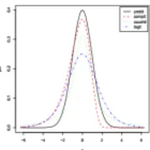
Figure 1. Densities corresponding to the link functions. The sim-ilarities are around the center of the distributions. Di¤erences can be seen at the tails
criticism of the overuse of the logit link function and a tendency to give it a place above the rest of existing link functions. In [7]’s own words: An unbelievably huge literature tried to establish a transcendental "law of logistic growth"; measured in appropriate units, practically all growth processes were supposed to be represented by a function of the form (1.3) with t representing time. Lengthy tables, complete with chi-square tests, supported this thesis for human populations, for bacterial colonies, development of railroads, etc. Both height and weight of plants and animals were found to follow the logistic law even though it is theoretically clear that these two variables cannot be subject to the same distribution. Laboratory experiments on bacteria showed that not even systematic disturbances can produce other results. Population theory relied on logistic extrapolations (even though they were demonstrably unreliable). The only trouble with the theory is that not only the logistic distribution but also the normal, the Cauchy, and other distributions can be …tted to the same material with the same or better goodness of …t. In this competition the logistic distribution plays no distinguished role whatever; most contradictory theoretical models can be supported by the same observational material.
As a matter of fact, it’s obvious from the plot of their densities for instance that the probit and logit are virtually identical, almost superposed one on top of the other. It is therefore not surprising that one would empirically notice virtually no di¤erence when the two are compared on the same binary regression task. Despite this apparent indistinguishability due to many of their similarities, it is fair to recognize that the two functions di¤erent, at least by de…nition and by their very algebra. [4] argue in their paper that probit and logit will yield di¤erent results in the multivariate context. Their work is a rarety in a context where most researchers seem to have settled comfortably with the acceptance of the fact that the two links are essentially the same from a utility perspective. For such researchers, using one over the other is determined solely by mathematical convenience and a matter of taste. We demonstrate both theoretically and computationally that they all predictively equivalent in the univariate case, but we also provide a characterization of the conditions under which they tend to di¤er in the multivariate context.
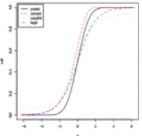
Figure 2. CDFs corresponding to the link functions. The simi-larities are around the center of the distributions. Di¤erences can be seen at the tails
Throughout this work, we perform model comparison and model selection using both Akaike Information Criterion (AIC) and Bayesian Information Criterion (BIC). Taking the view that the ability of an estimator to generalize well over the whole population, provides the best measure of it ultimate utility, we provide extensive comparisons of the performances of each link functions based on their corresponding test error. In the present work, we perform a large number of simulations in various dimensions using both arti…cial and real life data. Our results persistently reveal the performance indistinguishability of the links in univariate settings, but some sharp di¤erences begin to appear as the dimension of the input space (number of variables measured) increased.
The rest of this paper is organized as follows: section2presents some general de…nitions, namely our meaning of the terms predictive equivalence and structural equivalence, along with some computational demonstrations on simulated and real life data. This section also clearly describes our approach to demonstrating/verifying our claimed results. We show in this section, that for low to moderate dimensional spaces, goodness of …t and predictive performance measures reveal the equivalence between probit and logit. Section
3provides our formal proof of the equivalence of probit and logit. Section4reveals that there might be some di¤erences in performance when the input space becomes very large. Our demonstration in this section in based on the famous AT&T57-dimensional Email Spam Data set . Section5provides a conclusion and a discussion, along with insights into extensions of the present work.
2. Definitions, Methodology and Verification
Throughout this work, we consider comparing models both on the merits of goodness of …t, and predictive performance. With that in mind, we can then de…ne equivalence both from a goodness of …t perspective and also from a predictive optimality perspective.From a predictive analytics perspective for instance, an important question to ask is: given a randomly selected vectorx, what is the probability that the prediction made by probit will di¤er from the one made by logit? In other words, how often do the probit and logit link functions yield di¤erence predictions? This is particularly important in predictive analytics in the data mining and machine learning where the nonparametric nature of most models forces the experimenter to focus on the utility of the estimator rather than
its form. We respond to this need by de…ning what we call the100(1 )%predictive equivalence.
2.1. Basic de…nitions and results. Throughout this paper, X is used to denote the input space whileY = f0; 1gis used to denote the binary response (output) space. From the probabilistic/statistical perspective, X Y is the corresponding sample space from which the data setf(xi; yi); i = 1; ; ng is randomly collected for statistical learning purposes.
De…nition 1. (Binary classi…er) A (binary) classi…er h is de…ned as a function that maps elements of X to f0; 1g, or more speci…cally
h : X ! f0; 1g x7! h(x):
In the generalized linear model (GLM) framework, given a link function with corresponding cdf F ( ), a binary classi…er h under the majority rule takes the form
h(x) =1
2 1 + sign (x) 1
2 ;
where (x) = Pr[Y = 1jx] = F ( (x)), (x) is the linear component, and sign( ) is the signum function, namely 8w 2 IR,
sign(w) = 8 < : +1 w > 0; 0 w = 0; 1 w < 0: For instance, the logit binary classi…er is given by
hlogit(x) =
1
2 1 + sign ( (x)) 1
2 ;
and the the probit binary classi…er is given by hprobit(x) =
1
2 1 + sign ( (x)) 1
2 ;
where ( ) and ( ) are as de…ned in Table (1).
We shall measure the predictive performance of a classi…erhby choosing a loss function
`( ; ) and then computing the expected loss (also known as risk functional) R(h) as follows:
R(h) = E[`(Y; h(X))] = Z
X Y
`(y; h(x))p(x; y)dxdy:
Under the zero-one loss function `(Y; h(X)) = 1fY 6=h(X)g, the risk functional R(h) is the misclassi…cation rate, more speci…cally
R(h) = E[`(Y; h(X))] =
Z
In practice,R(h)cannot be computed in closed-form because the distribution of(X; Y )is unknown. We shall therefore use the so-called the average test error or average empirical prediction error as our predictive performance measure to compare classi…ers.
De…nition 2. (Average Test Error) Given a sample f(xi; yi); i = 1; ; ng, we
ran-domly form a training set f(x(tr)i ; y (tr)
i ); i = 1; ; ntrg and a test set f(x (te) i ; y
(te) i ); i =
1; ; nteg. We typically run R = 1000 replications of this split, with 2=3 of the data
al-located to the training set and 1=3 to the test set. The test error here under the symmetric zero-one loss is given by
^ Rtest(h) = TE(h) = 1 nte nte X i=1 1 fyi(te)6=h(x (te) i )g = #fy (te) i 6= h(x (te) i )g nte ;
from which the average test error of h over R random splits of the data is given by ATE(h) = 1 R R X r=1 TEr(h);
where TEr(h) is the test error yielded by h on the rth split of the data.
De…nition 3. (Predictively concordant classi…ers) Let h1and h2be two classi…ers de…ned
on the same p-dimensional input space X . We shall say that h1 and h2 are 100(1 )%
predictively concordant if 8X 2 X drawn according to the density pX(x),
Prhh1(X) 6= h2(X)
i
= :
In other words, h1 and h2 are 100(1 )% predictively concordant if the probability of
disagreement between the two classi…ers is . When = 0, we say that h1 and h2 are
perfectly predictively concordant.
De…nition 4. (Predictively equivalent classi…ers) Let h1 and h2 be two classi…ers de…ned
on the same p-dimensional input space X . We shall say that h1 and h2 are predictively
equivalent if the di¤ erence between their average test errors is negligible, i.e., ATE(h1)
ATE(h2).
Lemma 1. If X Logistic(0; 1), and Y =p8X, then Y approx
N (0; 1).
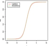
Proof. Graphical demonstration. Figure (3) below shows that the scaled version of the logistic cdf lines up almost perfectly with the standard normal.
Lemma 2. Let ( ) denote the standard normal cdf. Then
sign (z) 1 2 = sign r 8z 1 2 :
Proof. Straightforward from precious results.
Theorem 1. The probit and logit link functions are perfectly predictively concordant. Speci…cally, given an input space X and a density pX(x) on X ,
Prhhlogit(X) 6= hprobit(X)
i = 0;
Figure 3. Scaled version of the logistic CDF superposed on the standard normal CDF.
for all X 2 X drawn according to pX(x). Proof. For a givenX, LetEbe the event
E = sign ( (X)) 1
2 6= sign ( (X)) 1 2
we must show that = Pr[E] = 0. Based on Lemma (1), we can writeEas
E = sign r 8 (X) 1 2 6= sign ( (X)) 1 2 :
Then = Pr[E] = 0. Thanks to Lemma (2), it is straightforward to see that = 0. De…nition 5. Let M1 and M2 be two binary regression models based on two di¤ erent
link functions de…ned on the same p-dimensional input space. We shall say that M1 and
M2 are structurally equivalent if there exists a nonzero real constant 2 R such that (M1)
j
(M2)
j for all j = 1; ; p. In other words, the parameters of M1 are just a scaled
version of the parameters of M2, so that knowing the parameters of M1 is su¢ cient to
completely determine the parameters of M2, and vice-versa.
Theorem 2. The logit and probit models are structurally equivalent.
Proof. Thanks to Lemma (1), we can write
(x> (logit)) r 8x > (logit) = x> r 8 (logit) = (x> (probit)); where (probit) r 8 (logit) :
2.2. Computational Veri…cation via Simulation. To get deeper into how strongly related the probit and logit models are, we now seek to estimate via simulation, the constant coe¢ cient that relates their parameter estimates. Indeed, we conjecture that
^(logit) and ^(probit)are linearly related via the regression equation
^(probit)= + ^(logit)+ ;
where is the intercept and is the noise term. To estimate one instance of , we generate
M random replications of the dataset, and for each replication we estimate a copy of ^, and with it we also compute an estimate of = cor( ^(probit); ^(logit))the correlation coe¢ cient between ^(probit)and^(logit). By repeating the estimationRtimes, we gather data to determine the central tendency of and the corresponding correlation.
Algorithm 1.
For r = 1 to R
For s = 1 to S
– Generate a random replicate of f(xi; yi); i = 1; ; ng
– Estimate logit and probit coefficients ^(logit)s and ^ (probit) s
End
Store the simulated data D(r)= f(^(logit)s ; ^ (probit)
s ); s = 1; ; Sg
Fit M(r)
, the model ^(probit)s = + ^ (logit)
s + s using D(r)
Extract the coefficient ^(r) from M(r)
Compute ^(r) estimate of correlation between ^(probit) and ^(logit) End
Collect f^(r)and ^(r); r = 1; ; Rg, then compute relevant statistics.
Example 1: We consider a random sample of n = 199 observations f(xi; yi); i =
1; ; ng where the xi are equally spaced points in an interval [a; b], that is, xi =
a + b a
n 1 (i 1), and yi are drawn from one of the binary regression models. For instance, we set the domain ofxi to[a; b] = [0; 1]and generate theYi’s from a Cauchit model with slope1=2and intercept0, i.e.,Yi
iid Bernoulli( (xi)), with Pr[Yi= 1jxi] = (xi) = 1 tan 1 1 2xi + 2 ;
UsingR = 99replications each runningS = 199random samples, we obtain the following results, see Figure (4), (5), (6). The most striking …nding here is that the estimated coe¢ cient of determination is roughly equal to1, indicating that the knowledge of logit coe¢ cient almost entirely helps determine the value of the probit coe¢ cient. Hence our claim of structural equivalence between probit and logit. The value of the slope appears to be in the neighborhood of0:6.
Example 2: We now consider the famous Pima Indian Diabetes dataset, and obtain para-meter estimates under both the logit and the probit models. The dataset is7-dimensional, withx1= npreg,x2= glu,x3 = bp,x4 = skin,x5= bmi,x6= pedandx7= age.
Figure 4. Scatterplot of ^(probit) against ^(logit) based on the R replications generated
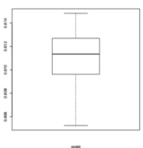
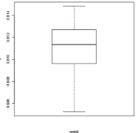
Figure 5. Boxplot of the R replications of the estimate of the coe¢ cient of determination between ^(probit) and ^(logit)
Figure 6. Boxplot of the R replications of the estimate of the coe¢ cient of determination between ^(probit) and ^(logit)
Under the logit model, the probability that patientihas diabetes given its characteristics
xi is given by
Pr[Diabetesi= 1jxi] = (xi) =
1 1 + e (xi);
where
(xi) = 0+ 1npreg + 2glu + 3bp + 4skin
Figure 7. Boxplot of the R replications of the estimate of the slope
We obtain the parameter estimates using R, and we display in the following table their values.
As can be seen in the Table (3), the ratio of the probit coe¢ cient over the logit coe¢ cient is still a number around0:6for almost all the parameter. Indeed, the relationship
^(probit)
j ' + 0:6^
(logit)
j +
appears to still hold true. The deviation from that pattern observed in variable skin is probably due to the extreme outlier in its distribution. It is important to note that although our theoretical justi…cation was built under the simpli…ed setting of a univari-ate model with no intercept, the relationship uncovered still holds true in a complete multivariate setting, with each predictor variable obeying the same relationship.
Example 3: We also consider the benchmark Crabs Leptograpsus dataset, and obtain para-meter estimates under both the logit and the probit models. The dataset is5-dimensional, withx1= F L,x2= RW,x3= CL,x4= CW andx5= BD. Under the logit model,
the probability that the sex of crabiis male given its characteristicsxiis given by Pr[sexi = 1jxi] = (xi) = 1 1 + e (xi); where (xi) = 0+ 1FL + 2RW + 3CL + 4CW + 5BD:
We obtain the parameter estimates using R, and we display in the following table their values.
As can be seen in the above Table (4), the estimate^of the ratio of the probit coe¢ cient over the logit coe¢ cient is still a number around0:6for almots all the parameter. Indeed, the relationship
^(probit)
j ' + 0:6^
(logit)
j +
appears to still hold true. It is important to note that although our theoretical justi-…cation was built under the simpli…ed setting of a univariate model with no intercept, the relationship uncovered still holds true in a complete multivariate setting, with each predictor variable obeying the same relationship.
Claim 1.
As can be seen from the examples above, the value of ^ lies in the neighborhood of 0:6, regardless of the task under consideration. This supports and con…rms our conjecture that there is a …xed linear relationship between probit coe¢ cients and logit coe¢ cients to the point that knowing one implies knowing the other. Hence, the two models are structurally equivalent. In a sense, wherever logistic regression has been used successfully, probit regression will do just as a job. This result con…rms what was already noticed and strongly expressed by [?] (pp 52-53).
2.3. Likelihood-based veri…cation of structural equivalence. In the proofs pre-sented earlier, we focused on the parameters and never mentioned their estimates. We now provide a likelihood based veri…cation of the structural equivalence of probit and logit. Without loss of generality, we shall focus on the univariate case where the un-derlying linear model does not have the intercept 0, so that (xi) = xi. With xi denoting the predictor variable for the ith observation, we have the probability model
Pr[Yi = 1jxi] = (xi) = F ( (xi)) = F ( xi). Let ^ (logit)
and ^(probit)denote the estimates of for the logit and the probit link functions respectively. Our …rst veri…-cation of the equivalence of the above link functions consists of showing that ^(logit)
and ^(probit) are linearly related through ^(probit) = + ^(logit)+ , with a coe¢ -cient of determination very close to 1and a slope that remains …xed regardless of the task at hand. We derive the approximate estimates of theoretically using Taylor series expansion, but we also con…rm their values computationally by simulation.
Theorem 3. Consider an i.i.d sample (x1; y1); (x2; y2); ; (xn; yn) where xi2 R is a
real-valued predictor variable, and yi2 f0; 1g is the corresponding binary response. First
consider …tting the probit model Pr[Yi = 1jxi] = (xi) = ( xi) to the data, and let
^(probit) denote the corresponding estimate of . Then consider …tting the logit model and Pr[Yi = 1jxi] = (xi) = 1=(1 + exp( xi)) to the data, and let ^
(logit)
denote the corresponding estimate of . Then,
^(probit)
' 0:625^(logit):
Proof. Given an i.i.d sample (x1; y1); (x2; y2); ; (xn; yn) and the model Pr[Yi =
1jxi] = (xi), the loglikelihood for is given by
`( ) = log L( ) = n X i=1 fyilog (xi) + (1 yi) log(1 (xi))g:
Under the logit link function, we have (xi) = 1=(1 + e xi). Now, using a Taylor series expansion around zero for the two most important parts of the loglikelihood function, we get @log( (xi)) @ = xi 2 x2i 4 + x4i 48 3 x6i 480 5 ; and @log(1 (xi)) @ = xi 2 x2i 4 + x4i 48 3 x6i 480 5 :
The derivative of the approximate log-likelihood function for the logit model is then given by `0( ) = n X i=1 yi xi 2 x2i 4 + x4i 48 3 x6i 480 5 + n X i=1 (1 yi) xi 2 x2i 4 + x4i 48 3 x6i 480 5 ;
which, upon ignoring the higher degree terms in the expansion becomes
`0( ) '
n
X
i=1
4yixi 2xi x2i : It is straightforward to see that solving`0( ) = 0for yields
^(logit)' 2 2 Pn i=1xiyi Pni=1xi Pn i=1x2i :
If we now consider the probit link function, we have (xi) = ( xi) = R xi 1 1 p 2 e 1 2z 2 . Using a derivation similar to the one performed earlier, and ignoring higher order terms, we get `0( ) = @`( ) @ ' n X i=1 yi c1xi 2c2 x2i + n X i=1 (1 yi) c1xi 2c2 x2i = n X i=1 2c1xiyi c1xi 2c2 x2i wherec1= 0:797885andc2= 0:31831. This leads to
^(probit)' c1 2c2 2Pni=1xiyi Pn i=1xi Pn i=1x2i :
It is then straightforward to see that
^(probit) ^(logit) ' c1 4c2 = 0:625; or equivalently ^(probit)' 0:625^(logit):
It must be emphasized that the above likelihood-based theoretical veri…cations are dependent on Taylor series approximations of the likelihood and therefore the factor of proportionality are bound to be inexact. It’s re-assuring however to see that our compu-tational veri…cation does con…rm the results found by theoretical derivation.
3. Similarities and Differences beyond Logit and Probit
Other aspects of our work reveal that the similarities proved and demonstrated above be-tween the probit and the logit link functions extend predictively to the other link functions mentioned above. As far as structural equivalence or the lack thereof is concerned, Ap-pendix A contains similar derivations for the relationship between cauchit and logit, and the relationship between compit and logit. As far as, predictive equivalence is concerned, we now present a veri…cation based on the computation of many replications of the test error.
3.1. Computational Veri…cation of Predictive Equivalence. We now computation-ally compare the predictive merits of each of the four link functions considered so far. To this end, we compare the estimated average test error yielded by the four link functions. We do so by running R = 10000 replications of the split of the data set into train-ing and test set, and at each iteration we compute the correspondtrain-ing test error for the
classi…er corresponding to each link functions. For one iteration/replication for instance,
^
Rtest( ^f(probit)), R^test( ^f(compit)), R^test( ^f(cauchit)) and R^test( ^f(logit))are the values of the test error generated by probit, compit, cauchit and logit respectively. After R
replications, we have R random realizations of each of those four test errors. We then perform various statistical calculations on theRreplications, namely median, mean, stan-dard deviation, kurtosis, skewness, IQR etc..., to assess the similarity and the di¤erences among the link functions. We perform the similarR replications for model comparison using both AIC and BIC.
Example 4: Veri…cation of Predictive Equivalence on Arti…cial Data: f(xi; yi); i =
1; ; ngwhere xi N ormal(0; 22)and yi 2 f0; 1g are drawn for a cauchy binary regression model with 0= 1and 1= 2, namelyYi Bernoulli( (xi))where
(xi) = Pr[Yi= 1jxi] = 1 h tan 1(1 + 2xi) + 2 i :
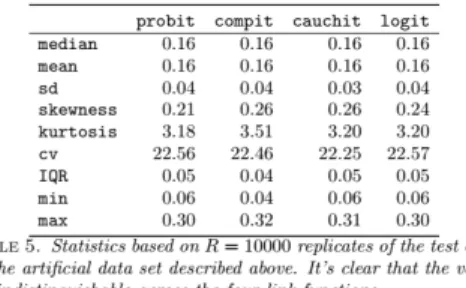
Table 5 shows some statistics on R = 10000replications of the test error. The above results suggest that the four link functions are almost indistinguishable as the estimated statistics are almost all equally across the examples.
Example 5: Veri…cation of Predictive Equivalence on the Pima Indian Diabetes Dataset: We once again consider the famous Pima Indian Diabetes dataset. The Pima Indian Diabetes Dataset is arguably one the most used benchmark data sets in the statistics and pattern recognition community. As can be see in Table 6, there is virtually no di¤erence between the models. In other words, on the Pima Indian Diabetes data set, the four link functions are predictive equivalent.
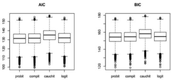
Figure 8. Comparative boxplots of both AIC and BIC across the four link functions based on R = 10000 replications of model …t-tings.
It’s also noteworthy to point out that all the four models also yield similar goodness of …t measures when scored using AIC and BIC. Indeed, Figure (7) reveals that over the
R = 10000replications of the split of the data into training and test set, both the AIC and BIC are distributionally similar across all the four link functions.
Despite the slight di¤erence shown by the Cauchit model, it is fair to say that all the link functions are equivalent in terms of goodness of …t. Once again, this is yet another evidence to support and somewhat reinforce/con…rm [7]’s claim that all these link functions are equivalent in terms of goodness of …t, and that the over-glori…cation of the logit model is at best misguided if not unfounded.
3.2. Evidence of Di¤erences in High Dimensional Spaces. Simulated evidence: We generates = 10000observations in the interval[ 15; 15]. For each link function, we compute the sign ofF (xi) 1=2for i = 1; ; s. We then generate a table containing the percentage of times the signs di¤er.
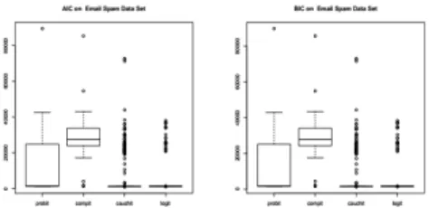
Computational Demonstrations on the Email Spam Data: Unlike all the other data sets encountered thus far, the email spam data set is a fairly high dimensional data set. It has a total ofp = 57variables andn = 4601observations.
Figure 9. Comparative Boxplots assessing the goodness of …t of the four link functions using AIC and BIC over R = 10000 repli-cations of model …tting under each of the link functions.
Clearly, the results depicted in Table 8 reveal some drastic di¤erences in performance among the four link functions on this rather high dimensional data. The boxplots below reinforce these …ndings as they show that in terms of goodness of …t measured through AIC and BIC, the compit model deviates substantially from the other models.
4. Conclusion and discussion
Throughout this paper, we have explored both conceptually/methodologically and com-putationally the similarities among four of the most commonly used link functions in bi-nary regression. We have theoretically shed some light on some of the structural reasons that explain the indistinguishability in performance in the univariate settings among the four link functions considered. Although section 2 concentrated mainly on the equivalence of the logit and probit, the Appendix provides a similar derivation for both the cauchit and the complementary log log link functions. We have also demonstrated by computa-tional simulations that the four link functions are essentially equivalent both structurally and predictively in the univariate setting and in low dimensional spaces. Our last example showed computationally that the four link functions might di¤er quite substantially when the dimensional of the input space becomes extremely large. We notice speci…cally that the performance in high dimensional spaces tends to defend on the internal structure of the input: completely orthogonal designs tending to bode well with all the perfectly sym-metric link functions while the non orthogonal designs deliver best performances under the complementary log log. Finally, the sparseness of the input space tends to dictate the choice of the most appropriate link function, Cauchit tending to be the model of choice
under high level of sparseness. In our future work, we intend to provide as complete a theoretical characterization as possible in extremely high dimensional spaces, namely pro-viding the conditions under which each of the link function will yield the best …t for the data.
5. Appendix A
Theorem 4. Consider an i.i.d sample (x1; y1); (x2; y2); ; (xn; yn) where xi2 R is a
real-valued predictor variable, and yi2 f0; 1g is the corresponding binary response. First
consider …tting the cauchit model Pr[Yi = 1jxi] = (xi) = 1 tan 1( xi) + 2 to the
data, and let ^(cauchit) denote the corresponding estimate of . Then consider …tting the logit model and Pr[Yi= 1jxi] = (xi) = 1=(1 + exp( xi)) to the data, and let ^
(logit)
denote the corresponding estimate of . Then, ^(cauchit)'
4^
(logit)
:
Proof. Given an i.i.d sample (x1; y1); (x2; y2); ; (xn; yn) and the model Pr[Yi =
1jxi] = (xi), the loglikelihood for is given by
`( ) = log L( ) = n X i=1 n yilog (xi) + (1 yi) log(1 (xi)) o :
For the Cauchit for instance, (xi) = 12 + 1tan 1( xi). We use the Taylor series expansion around zero for bothlog( (xi))andlog(1 (xi)).
log (xi) = log 2 + 2 xi 2 2x2i 2 2( 2 4) 3 x3i 3 3 + O(x 4 i) and log(1 (xi)) = log 2 2 xi 2 2x2 i 2 + 2( 2 4) 3x3 i 3 3 + O(x 4 i) A …rst order approximation of the derivative of the log-likelihood with respect to is
`0( ) = @`( ) @ = n X i=1 ( yi 2xi 4 x2i 2 + (1 yi) 2xi 4 x2i 2 ) = n X i=1 ( 4 xiyi 2 xi 4 2 x 2 i ) Solving`0( ) = 0yields ^ = 4 Pn i=1xiyi 2 Pn i=1xi 4 2 Pn i=1x2i which simpli…es to ^(cauchit)= 2 2Pni=1xiyi Pni=1xi Pn i=1x2i
References
[1] A. Armagan and R. Zaretzki. A note on mean-…eld variational approximations in bayesian probit models. Computational Statistics and Data Analysis, 55:641–643, 2011.
[2] S. Basu and S. Mukhopadhyay. Bayesian analysis of binary regression using symmetric and asymmetric links. Sankhya: The Indian Journal of Statistics, 62(3):372–387, 2000. [3] S. Chakraborty. Bayesian binary kernel probit model for microarray based cancer clas-si…cation and gene selection. Computational Statistics and Data Analysis, 53:4198– 4209, 2009.
[4] E.A. Chambers and D.R. Cox. Discrimination between alternative binary response models. Biometrika, 54(3/4):573–578, 1967.
[5] L. Csat´ o, E Fokou´ e, M Opper, B. Schottky, and O. Winther. E¢ cient approaches to gaussian process classi…cation. In S. A. Solla, T. K. Leen, and eds. K.-R. M¨ uller, editors, Advances in Neural Information Processing Systems, number 12. MIT Press, 2000.
[6] W. Feller. On the logistic law of growth and its empirical veri…cation in biology. Acta Biotheoretica, 5:51–66, 1940.
[7] W. Feller. An Introduction to Probability Theory and Its Applications, volume II. John Wiley and Sons, New York, second edition, 1971.
[8] G. D. Lin and C. Y. Hu. On characterizations of the logistic distribution. Journal of Statistical Planning and Inference, 138:1147–1156, 2008.
[9] S. Nadarajah. Information matrix for logistic distributions. Mathematical and Com-puter Modelling, 40:953–958, 2004.
[10] M. M. Nassar and A. Elmasry. A study of generalized logistic distributions. Journal of the Egyptian Mathematical Society, 20:126–133, 2012.
[11] M. Schumacher, R. Robner, and W. Vach. Neural networks and logistic regression: Part i. Computational Statistics and Data Analysis, 21:661–682, 1996.
[12] K. A. Tamura and V. Giampaoli. New prediction method for the mixed logistic model applied in a marketing problem. Computational Statistics and Data Analysis, 66:202– 216, 2013.
[13] A. van den Hout, P. van der Heijden, and R. Gilchrist. The Logistic Regression Model with Response Variables Subject to Randomized Response. Computational Statistics and Data Analysis, 51:6060–6069, 2007.
[14] D. Zelterman. Order statistics for the generalized logistic distribution. Computational Statistics and Data Analysis, 7:69–77, 1989.
Current address : Necla Gündüz: Fen Fakültesi, Istatistik Böl., Gazi Üniv., Ankara, Turkey E-mail address : [email protected]
Current address : Ernest Fokoué: School of Mathematical Sciences, Rochester Inst. of Tech., Rochester, New York 14623, USA