Indirect search for color octet muon at future muon colliders

(1)

MASTER OF SIENCE THESIS

SEPTEMBER 2020

INDIRECT SEARCH FOR COLOR OCTET MUON AT FUTURE MUON COLLIDERS

Thesis Supervisor: Dr. Ahmet Nuri AKAY Dariush MOHAMMADZADEH

(2)

(3)

iii

THESIS NOTIFICATION

I hereby declare that all the information in the thesis is obtained and presented within the framework of ethical behavior and academic rules. I also declare that the cited sources are fully cited, the references are fully stated, and that this thesis is also prepared in accordance with the TOBB ETU Institute of Natural and Applied Sciences writing rules.

(4)

(5)

v ÖZET Yüksek Lisans Tezi

RENK SEKİZLİSİ MUONUN GELECEKTEKİ MUON ÇARPIŞTIRICILARINDA DOLAYLI OLARAK ARANMASI

Dariush Mohammadzadeh

TOBB Ekonomi ve Teknoloji Üniveritesi Fen Bilimleri Enstitüsü

Mikro ve Nanoteknoloji Anabilim Dalı

Danışman: Dr. Ahmet Nuri Akay Tarih: Eylül 2020

SM fermiyon karışımları ve aile tekrarı, maddenin preonik bir yapıya sahip olması gerektiğini gösterir. ATLAS ve CMS deneylerinde, BSM parçacıkları geniş çapta incelenir. Bu parçacıkların tahmini, preonik modellerin önemli bir sonucu olarak düşünülebilir. Leptonların bileşik modellerde renk sekizlisi partnerlerine, l8, sahip olduğu tahmin edilmektedir. Bu parçacıklar, uyarılmış leptonlara ve leptoquarklara benzer. Öte yandan, muon çarpıştırıcıları, kurucu düzeyde bir çoklu-TeV ölçeğine ulaşmak için umut verici makineler olarak kabul edilir. Bu çalışmada, renk sekizlisi muonlar için gelecekteki muon çarpıştırıcılarının arama potansiyeli araştırılmıştır. Renk sekizlisi muonun, µ8, Lagranjiyen etkileşimi CalcHEP simülasyon programına eklenmiştir. Daha sonra, enine momentum ve pseudo-rapidity grafikleri üzerinde optimum kesmeleri (cuts) belirlemek için sinyal ve background işlemleri için farklı son durum dağılımları analiz edilmiştir. Son olarak, renk sekizlisi muon kütlesi üzerinde dışarlama (2σ), gözlem (3σ) ve keşif (5σ) limitleri elde etmek için istatistiksel anlamlılık analizi yapılmıştır. Analiz sonunda, 3.19 TeV, 6.65 TeV, 12.8 TeV, 25.9 TeV ve 135 TeV'ye kadar kütlelere sahip renk sekizlisi muonları, √s𝜇𝜇, sırasıyla, 1.5 TeV, 3 TeV, 6 TeV, 14 TeV ve 100 TeV olan muon çarpıştırıcılarında gözlemlenebilirliği gösterilmiştir. Sonuç olarak, gelecekteki muon çarpıştırıcılarının µ8 araştırması için büyük potansiyeli vardır.

(6)

(7)

vii ABSTRACT Master of Science Thesis

INDIRECT SEARCH FOR COLOR OCTET MUON AT FUTURE MUON COLLIDERS

Dariush Mohammadzadeh

TOBB University of Economics and Technology Institute of Natural and Applied Sciences Micro and Nanotechnology Science Programme

Supervisor: Dr. Ahmet Nuri Akay Date: September 2020

SM fermion mixings and family replication indicate that matter must have a preonic structure. In ATLAS and CMS experiments, BSM particles are widely studied. The prediction of these particles can be considered as a significant result of preonic models. Leptons are predicted to have color octet partners, l8, in composite models. These particles are similar to excited leptons and leptoquarks. On the other hand, muon colliders are considered as promising machines to achieve a multi-TeV scale at the constituent level. In this study, the search potential of future muon colliders for color octet muons was investigated.

The interaction Lagrangian of color octet muon, µ8, is implemented into the CalcHEP simulation program. Then different final state distributions for signal and background procedures have been analyzed to determine optimal cuts on transverse momentum and pseudo-rapidity. Finally, statistical significance analysis has been performed in order to obtain exclusion (2σ), observation (3σ), and discovery (5σ) limits on the mass of color octet muon.

It is shown that color octet muons with masses up to 3.19 TeV, 6.65 TeV, 12.8 TeV, 25.9 TeV, and 135 TeV can be observed at muon colliders with √s𝜇𝜇 equal to 1.5 TeV, 3 teV, 6 TeV, 14 teV and 100 TeV, respectively.

In conclusion, future muon colliders have huge potential for µ8 search. Keywords: Preonic models, Color octet muon, Muon colliders.

(8)

(9)

ix

ACKNOWLEDGEMENT

I would like to thank dear Prof. Dr. Ahmet Nuri Akay and Prof. Dr. Saleh Sultansoy who guided me with their valuable supports and scientific consultancy throughout my studies. Thanks to Dr. Mehmet Şahin from Uşak University for his wise experiences and scientific supports. I would like to thank my lovely wife and my parents for their help and supports for overcoming difficulties. And also thanks to TOBB University of Economics and Technology for M.Sc. scholarship and financial supports.

(10)

(11)

xi Page ÖZET ... vii ABSTRACT ... ix ACKNOWLEDGEMENT ... xi CONTENTS ... xiii

LIST OF FIGURES ... xvi

LIST OF TABLES ... xix

LIST OF ABBREVIATIONS ... xxi

LIST OF SYMBOLS ... xxiii

1. INTRODUCTION ... 1

2.THEORETICAL STUDIES ... 5

2.1 Systematics of Preon Models ... 5

2.1.1 Pati-Salam model ... 6

2.1.2 Fritzsch-Mandelbaum model (Haplon Model) ... 6

2.1.3 Matsushima model ... 7

2.1.4 Harari-Seiberg-Shube model (Rishon model) ... 7

2.1.5 Helon model ... 8

2.1.6 Preon Trinity model ... 9

2.1.7 Çelikel-Kantar-Sultansoy model ... 9

2.1.8 Fariborz-Jora-Nasri model ... 10

2.2 Minimal Fermion-Scalar Preon model ... 12

3. LHC AND FUTURE COLLIDER OPTIONS ... 15

3.1 Hadron Colliders ... 15 3.1.1 LHC ... 15 3.1.2 FCC ... 18 3.1.3 SppC ... 19 3.2 Electron-Positron Colliders ... 21 3.2.1 ILC ... 21 3.2.2 CLIC ... 22 3.2.3 PWFA-LC ... 24

(12)

xii

3.3 Muon Colliders ... 26

3.3.1 Advantages of muon colliders ... 26

3.3.2 Disadvantages of muon colliders ... 26

3.3.3 Different components of a muon collider ... 27

4. SEARCH FOR COLOR OCTET MUON AT FUTURE MUON COLLIDERS ... 31 4.1 Resonant Production ... 32 4.2 Pair Production ... 33 4.3 Indirect Production ... 34 5. CONCLUSION ... 47 REFERENCES ... 49 CURRICULUM VITAE ... 55

(13)

(14)

xiv

LIST OF FIGURES

Page

Figure 3.1 : Demonstration of the Large Hadron Collider ring [30] ... 16

Figure 3.2 : CERN’s accelerator complex [34] ... 17

Figure 3.3 : Location of FCC ring planned to be installed in the future [36] ... 19

Figure 3.4 : A hypothetical detector for the FCC-hh collider [37] ... 20

Figure 3.5 : A schematic view of SppC [38] ... 20

Figure 3.6 : Schematic layout of the ILC complex for 5 GeV center of mass energy (ILC TDR 2013) ... 21

Figure 3.7 : 3 TeV center of mass energy of CLIC layout [41] ... 23

Figure 3.8 : 8 Map showing the possible location for the CLIC accelerator [41] ... 23

Figure 3.9 : Arrangement of 10 TeV linear colliders based on PWFA ... 25

Figure 3.10 : Schematic layouts of Muon Collider complexes. ... 29

Figure 4.1 : Graph of decay width against the mass of 𝜇₈ at different compositeness scale ... 32

Figure 4.2 : Feynman diagram related to the resonant production of color octet muon ... 32

Figure 4.3 : Some Feynman diagrams related to the pair production of color octet muon ... 33

Figure 4.4 : Feynman diagram of indirect production of color octet muon at the muon colliders ... 34

Figure 4.5 : Distributions of indirect production cross sections according to mass of color octet muon at the three different muon colliders ... 34

Figure 4.6 : Distribution of indirect production cross sections according to mass of color octet muon at the muon colliders with √𝑠 = 100 TeV ... 35

Figure 4.7 : Dispersions of transverse momentum for final state jets at muon collider with √𝑠 = 1.5 TeV. ... 36

Figure 4.8 : Pseudo-rapidity dispersions of final state jets at muon collider with √𝑠 = 1.5 TeV... 36

(15)

xv

√𝑠 = 3 TeV. ... 37 Figure 4.11 : Dispersions of transverse momentum for final state jets at muon

collider with √𝑠 = 6 TeV. ... 38 Figure 4.12 : Pseudo-rapidity dispersions of final state jets at muon collider with

collider with √𝑠 = 14 TeV. ... 39 Figure 4.14 : Pseudo-rapidity dispersions of final state jets at muon collider with

collider with √𝑠 = 100 TeV. . ... 40 Figure 4.16 : Pseudo-rapidity dispersions of final state jets at muon collider with

√𝑠 = 100 TeV. ... 40 Figure 4.17 : The required integrated luminosity for the indirect exclusion,

observation, and discovery of 𝜇₈ for muon collider with √𝑠 = 1.5 TeV ... 42 Figure 4.18 : The required integrated luminosity for the indirect exclusion,

observation, and discovery of 𝜇₈ for muon collider with √𝑠 =3 TeV ... 42 Figure 4.19 : The required integrated luminosity for the indirect exclusion,

observation, and discovery of 𝜇8 for muon collider with √𝑠 = 6 TeV ... 43 Figure 4.20 : The required integrated luminosity for the indirect exclusion,

observation, and discovery of 𝜇₈ for muon collider with √𝑠 = 14 TeV ... 43 Figure 4.21 : The required integrated luminosity for the indirect exclusion,

(16)

(17)

xvii

LIST OF TABLES

Page

Table 1.1 : A summary history of searching for the basic structure of matter [1] ... 2

Table 2.1 : Quantum numbers of Fritzsch-Mandelbaum preons ... 7

Table 2.2 : Quantum numbers of preons in Rishon model ... 8

Table 2.3 : Standard Model Created With Helons ... 8

Table 2.4 : Possible electrical charges of preons for 𝑄_𝐹,𝑆 ≤ 1 status ... 10

Table 2.5 : Fariborz-Jora-Nasri Model preons and quantum numbers ... 11

Table 2.6 : Charges of other particles emerging from fermion-scalar models... 12

Table 2.7 : Two fermionic and one scalar preon state ... 13

Table 2.8 : Weak isotopic and hyper charges of preons belonging to minimal fermion-scalar model ... 14

Table 3.1 : Main parameters of LHC ... 18

Table 3.2 : Beam parameters of FCC proton-proton colliders ... 19

Table 3.3 : Main parameters of SppC ... 21

Table 3.4 : Main parameters of ILC ... 22

Table 3.5 : Main parameters of CLIC ... 24

Table 3.6 : Main parameters of PWFA-LC ... 25

Table 3.7 : Main parameters of muon colliders ... 29

Table 4.1 : The values of 1-year integrated luminosity for the muon colliders with different center-of-mass energies ... 35

Table 4.2 : Transverse momentum and Pseudo-rapidity cuts for muon colliders ... 41

Table 4.3 : Accessible mass values of color octet muon for indirect exclusion, observation, and discovery at different colliders. ... 44

(18)

(19)

xix

LIST OF ABBREVIATIONS

SM : Standart Model

DIS : Deep Inelastic Scattering BSM : Beyond the Standard Model ATLAS : A Toroidal LHC AparatuS CLIC : Compact LInear Collider CMS : Compact Muon Solenoid ERL : Energy Recovery Linac FCC : Future Circular Collider ILC : International Linear Collider LHC : Large Hadron Collider

LHeC : Large Hadron electron Collider

PWFA-LC : Plasma Wake Field Accelerator-Linear Collider SppC : Super proton-proton Collider

(20)

(21)

xxi

LIST OF SYMBOLS

The symbols used in this study are presented below with their descriptions.

Symbols Descriptions

𝜇8 Color Octet Muon

σ Beam Size

ε Constant Emittance

β D_e

Betatron Function

Electron Disruption Parameter

L Luminosity

PT Transverse Momentum

(22)

(23)

1 1. INTRODUCTION

What is the most basic thing in the universe? This is how people start to find the smallest building block of matter. The Sumerians, which existed about 6,000 years ago, believe that the universe is made up of two basic elements and that they are heaven and earth. When it comes to the ancient Greek ages, the universe is thought to consist of four basic structures. These are earth, fire, air, and water. In the middle ages, chemists found more substances, that is to say, elements and chemistry emerged. From the 19th century in the late 20th century, scientists conducted many experiments to question whether chemical elements have an internal structure. For the chemical properties of atoms, the concept of indivisible charge was put forward and this was called electron. 1897 J. J. Thomson after experiments on cathode rays, these rays were found to be composed of negatively charged electrons. The interpretation of Rutherford's alpha particles scattering back from a thin gold foil, the intense positive charge in the center of the atom, and it occupies an almost too small volume of the atom, was a turning point about the structure of the atom. Later, protons and neutrons that form the structure of the atom were found. With the development of particle accelerators in the 1950s, many different particles were found. These particles were called "particle zoo" particle garden. But in the 1960s, the famous scientist Murray Gell-Mann and George Zweig came up with a model that said the particles in this particle garden were made up of more basic particles. The particles predicted by this model are called quarks. Today there are many particles that we assume basically and understand Standard Model (SM) interactions: leptons, quarks, intermediate bosons, Higgs bosons. Therefore, the SM particles may consist of more basic elements. The subject of this thesis is to determine the potential of the colliders, which are intended to be established and which will be established in the future, to search for the color octet muon, which is one of the particles envisaged by the models for searching the most basic building block of matter.

Experimentally tested minimal SM contains 61 basic particles and 26 free parameters (Dirac neutrinos). With this multiplicity of particles, SM cannot end the story in

(24)

2

searching for the most basic particles or particles, and it is clear that we need a more fundamental theory. We have encountered this situation twice in the past. The last 150 years of searching for the basic building blocks of matter are summarized in Table 1.1. The first is the abundance of chemical elements, and the second is the hadron abundance that results in the quark model.

The first case is explained by the Rutherford experiment, while the second case is clarified by the Deep Inelastic Scattering (DIS) test in SLAC. At the point we have reached today, we are again faced with the excess of the number of elementary particles of the best model (SM) we have. This ongoing similarity indicates that SM fermions have a more basic structure or structures.

Table 1.1 A summary history of searching for the basic structure of matter [1]

Stages 1870-1930s 1950-1970s 1970-2020s

Fundamental

Constituent Inflation Chemical Elements Hadrons Quarks, Leptons

Systematics Periodic Table Eight-fold Way Family Replication

Confirmed Predictions New Elements New Hadrons New Particles?

Clarifying Experiments Rutherford SLAC, DIS LHC? FCC/SppC?

Building Blocks Proton, Neutron,

Electron Quarks Preons?

Energy Scale MeV GeV TeV?

Impact on Technology Exceptional Indirect Exceptional?

There are two main approaches to the existence of more basic structures: Super String and Composite Models. In terms of the simplification mentioned above, the composite models seem very interesting. These models try to explain nature with its most basic building blocks. Here, we are looking for composite, preon models, SM family replication, and fermion mixtures. These mixtures can be considered as a sign of the

(25)

3

(composite) are quite popular. For example, preon models predict particles such as excited leptons, excited quarks, diquarks, dileptons, leptoquarks, leptogluons, etc. Although leptogluones are in the same condition as excited leptons and leptoquarks, there is no direct research of them in ATLAS and CMS experiments on the Hadron Collider in CERN.

(26)

(27)

5 2.1. Systematics of Preon Models

Preons were first introduced by Jogesh Pati and Abdus Salam. In principle, composite models can be addressed in four stages (in general, each stage includes the previous one):

i) Composite Higgs bosons ii) Composite quarks and leptons iii) Composite W and Z bosons iv) Composite photon and gluons

The most common example of the first stage is Technicolor models. While this model naturally adds mass to W and Z bosons, it presents serious problems in massing quarks and leptons. Therefore expanded technicolor models were proposed. However, extended models disrupt the harmony of the main approach. Therefore, these models will not be dealt with within the thesis.

As for the second stage, the Preon models proposed to date can be divided into two main classes:

- Fermion-scalar models (FS) - 3-fermion models (FFF)

These models anticipate many new particles containing unusual quantum numbers. If the third stage occurs in nature, particles such as excited W and Z, color octets W and Z, scalar W, and Z are also envisioned.

The realization of the fourth stage does not seem natural with today's information because the photons and gluons are massless and correspond to intact adjustment symmetry.

(28)

6

Preon models have been developed since the 1970s [2-8]. Preon models proposed until the 1990s were collected in a book [9]. The perception of inter-family mixtures of quarks and leptons with the presence of at least three fermion families led to the idea that they may consist of more basic components. Particles that are more basic than quarks and leptons are called preons. The word Preon is used in particle physics for point particles, which are the subcomponents of quarks and leptons [2]. Since preons are more fundamental particles than quarks and leptons, their size should also be smaller than quarks and leptons. So their size should be less than 10−18_{cm. According} to some of the composite models, preons form leptons and quarks as connected states through a force similar to the Quantum Color Dynamics (QCD).

Some of the preonic models proposed to date are listed below. 2.1.1 Pati-Salam model:

It is an example of a fermion-scalar model. The color interactions in which SU(3)C and U(1)Y are subgroups based on the combination of quarks and leptons in the SU(4)C extended group (the number of leptons is considered the 4th color). The general setting group is SU(4)C×SU(4)L×SU(4)R. Three types of preon quads are used here: iL, R , and α. i = P, Π, λ, χ are right-handed and left-handed fermionic spin-1/2 quadruples, α = a, b, c, d are a bosonic spin-0 color quartet. a, b and c correspond to 3 main colors, as in the standard module, while d is associated with leptons. Quarks and leptons are connected states of fermions and scalar preons:

Ψ_𝐿,𝑅 = [ P Π λ χ ] L,R ⊗ (𝑎, 𝑏, 𝑐, 𝑑) = [ P𝑎,𝑏,𝑐 P𝑑 Π𝑎,𝑏,𝑐 Π𝑑 λ_{𝑎,𝑏,𝑐} λ_𝑑 χ𝑎,𝑏,𝑐 χ𝑑]_L,R = [ u𝑎,𝑏,𝑐 ν𝑒 d_{𝑎,𝑏,𝑐} 𝑒 𝑠𝑎,𝑏,𝑐 𝜇 c𝑎,𝑏,𝑐 𝜈𝑒 ] L,R

2.1.2 Fritzsch-Mandelbaum model: (Haplon model)

It is a fermion-scalar model prototype and has a hyper-color adjustment group [4]. This group is represented by SU(N). Table 2.1 shows the quantum numbers of the preons predicted by the model. Using these features, if we express the first family leptons and quarks through preons;

(29)

7

𝛽 −𝑒 2⁄ 𝑁 3 1/2

𝑥 𝑒 6⁄ 𝑁̅ 3 0

𝑦 −𝑒 2⁄ 𝑁̅ 3̅ 0

Similarly, adjustment bosons of weak interactions are expressed in terms of preons below:

𝑊+ = (𝛼𝛽̅) , 𝑊− = (𝛼̅𝛽) , 𝑍 = 1

√2(𝛼𝛼̅ + 𝛽𝛽̅)

In this model, gluons, photons, and hyper bosons are considered to be basic particles. 2.1.3 Matsushima model:

It is a fermion-scalar model. SU(3)_C× SU(2)_L× SU(2)_R is the basic representation of Matsushima and it uses the spin-0 preon and spin-1/2 preon supersymmetric pairs, each of which has a charge of e/6. Because the GL and GR bonding coefficients are independent of each other, the Λ_L compositeness scale is near the Fermi scale, and Λ_R is near the grand unified theory (GUT).

2.1.4 Harari-Seiberg-Shube model (Rishon model):

This model is a prototype model using only the fermionic preons (three fermion model) [3]. Two types of preons are used here: T with an electrical charge of e / 3 and V with an electrical charge of 0. The SU(3) color and SU(3) quantum numbers related to these preons are listed in Table 2.2. In the model, the representations that make up leptons and quarks can be separated as follows:

(30)

8

Table 2.2 Quantum numbers of preons in Rishon model

Preon Electrical charge

Hyper Color

Charge Color Charge Spin

T e/3 3 3 1/2

V 0 3 3̅ 1/2

The representation of the first family fermions in terms of preons according to this model is as follows [3, 10-12]:

𝑒+ = (𝑇𝑇𝑇), 𝜈 = (𝑉𝑉𝑉), 𝑢 = (𝑇𝑇𝑉), 𝑑̅ = (𝑇𝑉𝑉) 2.1.5 Helon model:

This model is based on Rishon model and it is three fermion model. The particle that is equivalent to the preon is called helon in this model. In the Helon model, 3 basic particles with +e/3, 0, and −e/3 are suggested, shown as H+_{, H}0_{, H}−_{respectively.} The helon infrastructure of the 1st family fermions of the Standard Model is given in Table 2.3.

Table 2.3 Standard Model Created With Helons

H₊ H₀ H₋ H₊H₊ e+ _u b - H+H0 ug d̅ r - H0H+ ur d̅̅̅ g - H0H0 d̅̅̅ b 𝑣𝑒 db H0H− - dg u̅ r H−H0 - u̅̅̅ g dr H−H− - u̅̅̅ b e−

(31)

9

named with 𝛼, 𝛽, and 𝛿, while bosonic ones are represented by the symbols 𝑥, 𝑦, and 𝑧. Spin-1/2 preons, 𝛼, 𝛽, and 𝛿 have a load of +1/3, -2/3, +1/3, respectively. Spin-1 anti-dipreons are in the form of:

𝑥 = (𝛽𝛿̅̅̅̅), 𝑦 = (𝛼𝛿̅̅̅̅), 𝑧 = (𝛼𝛽̅̅̅̅)

And their loads are given as +1/3, -2/3, +1/3 respectively. In this model; 𝑒− = (𝛽𝑥̅), 𝜈𝑒 = (𝛼𝑥̅), 𝑢 = (𝛼𝑥), 𝑑 = (𝛼𝑦), 𝑍 = (𝛼𝛼̅) and 𝑊− = (𝛽𝛼̅) Are as above.

2.1.7 Çelikel-Kantar-Sultansoy model:

While making this model, two assumptions were made: i) The statistics did not deteriorate, ii) The preons were colored. The first assumption is that the Standard Model fermions should include an odd number of fermionic preons. Therefore, either the fermion-scalar model or three fermion models are possible [8]. According to the second assumption, preons are considered to be particles of a color triad.

Leptons in the fermion-scalar model are composed of a fermionic preon and a scalar anti-preon,

𝑙 = (𝐹𝑆̅) = 1 ⊕ 8

Thus, each Standard Model lepton has one color octet pair. The color separation in three fermion models is as follows.

𝑙 = (𝐹𝐹𝐹) = 1 ⊕ 8 ⊕ 8 ⊕ 10

It is envisaged that two color octets and one color decouplet are the partners of each Standard Model lepton.

Within the framework of the fermion-scalar model, anti-quarks consist of a fermionic and a scalar type preon. Thus, one color sixtet is partner of each Standard Model:

(32)

10 Quarks in three fermion models:

𝑞 = (𝐹𝐹̅𝐹) = 3 ⊕ 3̅ ⊕ 6̅ ⊕ 15

have a composite structure. Thus, each Standard Model quark has one anti-triplet, one anti-sixtet, and one15-plet partner.

Different options for possible electric charges of color triple preons (𝑄𝐹,𝑆 ≤ 1) are given in Table 2.4. The fourth column corresponds to the Fritzsch-Mandelbaum model [4], there is a fermion-scalar symmetry in terms of electric charge in the fifth column, and this may be a sign of preonic supersymmetry.

Table 2.4 Possible electrical charges of preons for 𝑄𝐹,𝑆 ≤ 1 status [8]

Model 1 Model 2 Model 3 Model 4 Model 5

𝑆₁ 0 1/3 1/2 2/3 1

𝐹₁ 0 1/3 1/2 2/3 1

𝐹₂ -1 -2/3 -1/2 -1/3 0

𝑆₂ 1/3 0 -1/6 -1/3 -2/3

Within the framework of the fermion-scalar model, at least two fermions and two scalar type preons are needed to create the first family fermions of the Standard Model. Thus, the fermions of the first family

𝜈_𝑒 = (𝐹₁𝑆̅ ), 𝑒 = (𝐹₁ ₂𝑆̅ ); ₁ 𝑑̅ = (𝐹₁𝑆₂), 𝑢̅ = (𝐹₂𝑆₂) can be written as linked situations [8].

2.1.8 Fariborz-Jora-Nasri model:

This model envisions two fermionic preons, called psions ψ and chions χ [14]. This model has the global U(1)_V× U(1)_A× SU(2)_L× SU(2)_R symmetry. This symmetry is then reduced to SU(2)L× U(1)Y . Quantum numbers of the preons proposed in Table 2.5 are given.

(33)

11

ψR 2/3 0 1/2 3 + 6∗

χ_L -1/3 -1/2 0 3 + 6∗

χ_R -1/3 0 -1/2 3 + 6∗

After symmetry diffraction from the large group to the electro-weak group, the hypersomes of the preons; Y = 2 (Q − T3L), Y (ψL) = 1/3, Y (ψR) = 4/3, Y (χ_L) = − 1/3, Y (χ_R) = − 2/3. The actual value should be Y (χ_L) = 1/3. In the study, it is said that the scalar singles will be related to the symmetry diffraction of the electron weak group, and the scalar pairs are defined as follows.

(χR † _ψ L χ_R† ψ_L) Y = 1; ( ψ_R† ψ_L ψ_R† χ_L) Y = −1 In this model, leptons are made as follows.

eL = ψL † ψ_L†χ_L†, eR = ψR † ψ_R†χ_R†, υL= χL † χ_L†ψ_L†, υR = χR † χ_R†ψ_R†

First family leptons are given with 3 × 3 × 3, second family leptons with 6∗_{× 6}∗_× 6∗ and third family leptons with 3 × 3 × 6∗.

Quarks are constructed as follows. uL= χL † χLψL, uR= χR † χRψR, dL= ψL † χLψL, dR= ψR † χRψR

First family quarks are given with 3∗× 3 × 3, second family quarks with 6 × 6∗× 3 and third family quarks with 3∗× 3 × 6∗ or 6 × 3 × 3.

So far, some of the preonic models proposed in previous years have been summarized. Today, interest in preonic models is increasing. There are many studies on diquarks, excited fermions, leptoquarks, leptogluons envisaged in preonic models [15-24]. The above-mentioned models (and preon models in general) have two shortcomings in the basics: the preon level interaction dynamics are unknown and the number of preons is high given the SM families. The first of these shortcomings can be eliminated as a result of experimental observation of preons and their interactions. The second

(34)

12

shortcoming can be overcome thanks to the new level of prepreonic structure, which will allow reducing the number of key elements.

2.2. Minimal Fermion-Scalar Preon Model:

The common problems of the above-mentioned models are the emergence of other particles that have not yet been observed at the SM level. For example, in the fermion-scalar models of color triplet preons, the following particles appeared in addition to the first SM family fermions. These are as color singlets:

(𝐹₁𝑆̅ ) and (𝐹₂ ₂𝑆̅ ) ₂ And are as color triplets:

(𝐹₁𝑆̅ ) and (𝐹₁ ₂𝑆̅ ) ₁

The electrical charges of these particles are shown in Table 2.6.

Table 2.6 Charges of other particles emerging from fermion-scalar models additional

particles

Electrical Charges

Model 1 Model 2 Model 3 Model 4 Model 5

(𝐹1𝑆̅2) -1/3 1/3 2/3 1 5/3

(𝐹₂𝑆̅₂) -4/3 -2/3 -1/3 0 2/3

(𝐹̅1𝑆̅1) 0 -2/3 -1 -4/3 -2

(𝐹̅₂𝑆̅₁) 1 1/3 0 -1/3 -1

The problem arises that the particles in question have not yet been discovered or their masses are more than the SM mass scale. Fritzsch and Mandelbaum give a solution for above-mentioned problem [4] by proposing QED or QCD-like preon dynamics (hyper color). Impulsive interactions between the same hyper colored preons eliminate these undesirable connected states. But in these models, S₁ is a color anti-triplet; F₁, F₂ and S2 are randomly trio of colors. In addition, preon dynamics do not have to be QED or QCD like.

By considering the problem mentioned above, a minimal fermion scalar model is proposed that prevents the emergence of unwanted particles [1]. The colors, loads, and spins of the proposed preons are given in Table 2.7.

(35)

13

𝐹₁_𝐿,𝑅 3 1/6 1/2

𝐹₂_𝐿,𝑅 3 -5/6 1/2

𝑆 3 1/6 0

Thus, the bound states of F₁ and F₂ with S form only the SM fermions. For example: 𝑄_𝐹̅̅̅₂ + 𝑄𝑆̅ = + 2 3; 𝐶𝐹̅̅̅2⊗ 𝐶𝑠̅ = 3̅ ⊗ 3̅ = 3 ⊕ 6̅ → 𝑢 = (𝐹̅̅̅𝑆̅)2 3 𝑄𝐹̅̅̅1 + 𝑄𝑆̅ = − 1 3; 𝐶𝐹̅̅̅1⊗ 𝐶𝑠̅ = 3̅ ⊗ 3̅ = 3 ⊕ 6̅ → 𝑑 = (𝐹̅ 𝑆̅)1 3 𝑄_𝐹₁+ 𝑄_𝑆̅ = 0 ; 𝐶_𝐹₁ ⊗ 𝐶_𝑠̅ = 3 ⊗ 3̅ = 1 ⊕ 8 → 𝑣_𝑒 = (𝐹₁𝑆̅)₁ 𝑄_𝐹₂ + 𝑄_𝑆̅ = −1; 𝐶_𝐹₂ ⊗ 𝐶_𝑠̅ = 3 ⊗ 3̅ = 1 ⊕ 8 → 𝑒− _{= (𝐹} 2𝑆̅)1

It is clear from here that the proposed model predicts the presence of color octet leptons and color sixtet antiquarks.

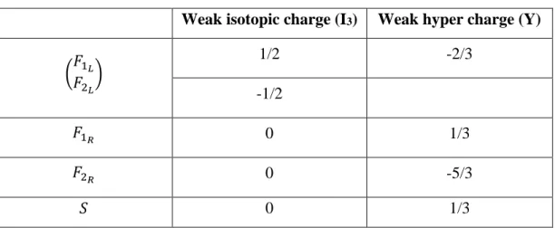
Color triplet preons within the framework of fermion-scalar model imply that the QCD will occur at the preonic level. Also, no change in space-time structure is a sign of the occurrence of the electro-weak tuning symmetry at the preonic level. The weak iso-spin and weak hyper charges of the preons of the model have been foreseen in Table 2.8 are shown.

Another important issue is family repetition. The second and third SM fermion families may occur by quantum double stimuli [25].

For instance, adding an (𝑆𝑆̅) to the first SM fermion family make the second and third family fermions, as shown below.

𝜈_𝜇 = (𝐹₁𝑆̅)(𝑆𝑆̅) 𝜇 = (𝐹₂𝑆̅)(𝑆𝑆̅) 𝑠 = (𝐹̅ 𝑆̅)(𝑆𝑆̅) 𝑐 = (𝐹₁ ̅̅̅𝑆̅)(𝑆𝑆̅) ₂ 𝜈𝜏 = (𝐹1𝑆̅)(𝑆𝑆̅)2 𝜏 = (𝐹2𝑆̅)(𝑆𝑆̅)2 𝑏 = (𝐹̅ 𝑆̅)(𝑆𝑆̅)1 2 𝑡 = (𝐹̅̅̅𝑆̅)(𝑆𝑆̅)2 2

(36)

14

Table 2.8 Weak isotopic and hyper charges of preons belonging to the minimal fermion-scalar model

Weak isotopic charge (I3) Weak hyper charge (Y)

(𝐹1𝐿 𝐹2𝐿 ) 1/2 -2/3 -1/2 𝐹1𝑅 0 1/3 𝐹2𝑅 0 -5/3 𝑆 0 1/3

In the above structure (𝑆𝑆̅) it is assumed that only the single component is involved in the formation of the 2nd and 3rd family SM fermions. On the other hand, it can be considered that the formation of upper families contains the color octet component of (𝑆𝑆̅). In this case, (𝐹𝑆̅) (𝑆𝑆̅) will have a color structure as follows:

(1 ⊕ 8) ⊗ (1 ⊕ 8) = 1 ⊕ 8 ⊕ 8 ⊕ 1 ⊕ 8 ⊕ 8 ⊕ 10 ⊕ 10̅̅̅̅ ⊕ 27

Thus, the first single muon can be thought of as the second single tau. In consequence, the muon has two color octets, while the tau has two color octets, a color decouplet, an anti-color decouplet, and a 27-plet pair. The same structure can be considered for muon and tau neutrino.

The considerable point is that the minimal fermion-scalar preon model contains, in principle, a triangular anomaly that can be eliminated by handling the same fermionic preons, as in other FS models.

(37)

15

3. LHC AND FUTURE COLLIDER OPTIONS

Current and future collider options, in which we will identify the research potential of the color octet muon, are discussed in this section.

3.1 Hadron Colliders 3.1.1 LHC

The Large Hadron Collider (LHC) is the largest and most powerful particle accelerator (LHC 2018) in the world currently in operation. It first started working on September 10, 2008. The LHC consists of a 27 kilometer long ring and a series of accelerators to increase the energy of the particles.

Before colliding, two beams of high energy particles are accelerated at a speed close to the speed of light. Bundles move in the opposite direction in separate bundle pipes and these bundle pipes are kept under a very high vacuum. Then superconducting electromagnets provide a strong electromagnetic field to guide these bundles around the accelerator ring. Electromagnets are made of special electrical cables with efficient electrical conductors, without resistance or energy loss, operating in a superconducting state. These magnets must be cooled to a temperature that is cooler than empty space, i.e. -271.3 ° C. The magnets and other systems of accelerator are cooled by a liquid helium distribution system.

Thousands of different kinds and sizes of magnets are used to guide the beam around the accelerator. These are 392 quadruple magnets that bend bundles and focus on 1232 bipolar magnets, each 15 m long, and 5-7 m long bundles each. Just before the collision, different types of magnets bring the particles closer together to increase the probability of collision.

The seven experiments in the LHC ring use individual detectors to analyze the countless particles produced by collisions. These experiments are conducted in collaboration with scientists from institutes all over the world. Each experiment pursues a different purpose and is characterized by its perceiver.

(38)

16

The largest of these detectors are ATLAS [26] and CMS [27] and they were set up for general particle physics research. These two independents, designed independently, are crucial for mutual approval of new discoveries. The heavy-ion detector ALICE [28], built for some more specific purposes, is designed to study the physics of the substance that interacts strongly with extreme energy densities where a phase of the substance is called quark-gluon plasma occurs. LHCb [29] investigates substance and antimatter asymmetry by examining b and c quarks. These four great subordinates are located in large caves on the LHC ring. The positions of the LHC 4 large detector are shown in Figure 3.1.

Figure 3.1 Demonstration of the Large Hadron Collider ring [30]

Smaller experiments in the LHC, TOTEM focusing on forwarding particles (collision at small angles) and cosmic in laboratory conditions LHCf [31], which uses collisions in the LHC to simulate rays. TOTEM uses the detectors on both sides of the CMS interaction point, while the LHCf consists of two detectors located 140 meters on either side of the ATLAS collision point along the LHC bundle line. MoEDAL [32] uses detectors located near the LHCb to search for the magnetic single pole (a hypothetical particle with a magnetic charge).

The LHC's proton source is hydrogen gas in an enclosed chamber [33]. An electric field is used to separate the hydrogen gas from its electrons, which will produce

(39)

17

GeV. Following this, protons enter Proton Synchrotron (PS), which will increase their energy to 25 GeV. From here, protons are sent to the Super Proton Synchrotron (SPS) and their energy is increased to 450 GeV.

Figure 3.2 CERN’s accelerator complex [34]

These protons with 450 GeV energy are transferred to two separate bundles of LHC. These two bundles rotate in opposite directions. Figure 3.2 shows the accelerator chain that delivers protons to the required energy. The time taken to fill each LHC ring is 4 minutes 20 seconds, and after 20 minutes both beams reach 6.5 TeV, their highest energy. The bundles circulate in LHC rings for hours under normal operating conditions. In cases where the total energy is equal to 13 TeV (LHC's planned bundle energy is 7 TeV.), ALICE, ATLAS, LHCb, and CMS are involved in a collision. The basic parameters of these colliding beams are shown in Table 3.1.

(40)

18 Table 3.1 Main parameters of LHC

Beam Energy (TeV) 6.5 (7)

Peak Luminosity (1034 cm-2 s-1) 10.0 Particles Per Bunch (1011₎ ₁ Norm. Transverse Emittance (μm) 3.75

Beta-value at I.P. 𝛽∗_(m) _0.50 Beam Size (μm) 15.9 Number of Bunches 2808 Bunch Spacing (ns) 25 Bunch Length (mm) 77 Beam-Beam Parameter 3.42 × 10−3 3.1.2 FCC

The future Circular Collider's hadron-hadron option (FCC-hh) aims to provide a proton-proton collision at almost a degree higher energy than LHC. The targeted mass center energy is 100 TeV. Nb3Sn-based advanced superconducting magnets are needed in accelerators to provide this level of the center of mass energy. Assuming that the nominal dipole magnetic field is 16 T, it is clear that such a machine will have a circumference of 100 km. The FCC is expected to provide 20 ab-1 total irradiation over a 25-year period in both main experiments.

The Future Circular Collider (FCC) is planned to be established in CERN as the forward link of LHC, as in Figure 3.3 [35, 36]. The FCC, which aims to accelerate the protons from LHC to 50 TeV, is expected to play a major role in the search for new physics.

The planned proton beam parameters of the FCC are given in Table 3.2. In Figure 3.4, it is planned to be established on the FCC ring and in search of new physics. A hypothetical design of the perceived great role plays a design. The diameter of the sensor in the design is 20 m and the length is 50 m.

(41)

19

Figure 3.3 Location of FCC ring planned to be installed in the future [36]

Table 3.2 Beam parameters of FCC proton-proton colliders

Baseline Nominal

Beam Energy (TeV) 50 50

Peak Luminosity (1034 cm-2 s-1) 5.0 < 30

Particles Per Bunch (1010) 10 10

Norm. Transverse Emittance (μm) 2.2 2.2

Beta-value at I.P. 𝛽∗ (m) 1.1 0.3 Beam Size (μm) 6.8 3.5 Number of Bunches 10400 10400 Bunch Spacing (ns) 25 25 Bunch Length (mm) 80 80 3.1.3 SppC

Super Proton-Proton Collider (SppC) is a proton-proton collider planned to be installed in China with 71.2 TeV and 136 TeV mass center energy options .

It is stated that in such a collider, electron-positron and proton-proton collisions can be done simultaneously and provide complementary information.

(42)

20

Figure 3.4 A hypothetical detector for the FCC-hh collider [37] Besides, electron-proton collisions can be made using both machines.

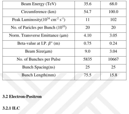
In early 2014, IHEP decided to prepare and publish a conceptual report within a year for CEPC-SppC to take part in the next 5-year plan of the Chinese Government. The report includes a 54 km ring design. This design was kept at this size due to cost anxiety. An alternative ring design of 100 km length is also included in the report. A schematic representation of SppC is given in Figure 3.5 [38] and the bundle parameters that it will have are given in Table 3.3.

(43)

21

Peak Luminosity(1034_cm-2_s-1₎ ₁₁ ₁₀₂ No. of Paricles per Bunch (1010₎ ₂₀ ₂₀ Norm. Transverse Emittance (μm) 4.10 3.05

Beta-value at I.P. 𝛽∗_(m) _0.75 _0.24

Beam Size(μm) 9.0 3.04

No. of Bunches per Pulse 5835 10667

Bunch Spacing(ns) 25 25

Bunch Length(mm) 75.5 15.8

3.2 Electron-Positron 3.2.1 ILC

The International Linear Collider (ILC) is a linear electron-positron collider based on 1.3 GHz superconducting radio frequency (SCRF) acceleration technology. It is designed to reach 200-500 GeV (which can be increased up to 1 TeV) mass center energy with high luminosity. A schematic representation of the ILC complex is given in Figure 3.6.

Figure 3.6 Schematic layout of the ILC complex for 5 GeV center of mass energy (ILC TDR 2013)

(44)

22

Top-level parameters for the baseline operational range of mass center energies from 200 to 500 GeV are optimized to provide maximum achievable physics performance with relatively low risk and minimal cost. The main parameters of the 200, 250, 350, and 500 GeV center of mass ILC are shown in Table 3.4.

Table 3.4 Main parameters of ILC

Beam Energy (GeV) 100 125 175 250

Luminosity (1034 cm-2 s-1) 0.56 0.75 1.0 1.8 Proposed site length (km) 30.5 30.5 30.5 30.5 Unloaded / loaded gradient (MV/m) 31.5 31.5 31.5 31.5

Beam power (MW) 2.1 2.6 3.7 5.3

No. of particles per bunch (109) 2.0 2.0 2.0 2.0 Input transverse horizontal emittance (norm.)

(nm) 10 10 10 10

Input transverse vertical emittance (norm.) (nm) 35 35 35 35 Nominal horizontal IP beta function (mm) 16 13 16 11 Nominal vertical IP beta function (mm) 0.34 0.41 0.34 0.48 Horizontal IP beam size before pinch (nm) 904 729 684 474 Vertical IP beam size before pinch (nm) 7.8 7.7 5.9 5.9 No. of bunches per pulse 1312 1312 1312 1312

Linac repetition rate (Hz) 5 5 5 5

Bunch train length (ns) 554 554 554 554

Bunch separation (ns) 8 8 8 8

Bunch length (mm) 0.3 0.3 0.3 0.3

There are two question marks ahead of the construction of the ILC: finding and financing a host country for the project. Japan is among the countries that are candidates to host the collider.

3.2.2 CLIC

After preliminary physics studies based on an electron-positron collider in several Multi-TeV energy ranges [39,40], CLIC studies focused on the design of a linear collision with 3 TeV mass collision energy [41]. The luminosity for this collider is planned as 5.9 × 1034 cm-2 s-1. The elements that make up the CLIC technology are

(45)

23

Figure 3.7 3 TeV center of mass energy of CLIC layout [41]

(46)

24 Table 3.5 Main parameters of CLIC

Beam Energy (GeV) 1500

Luminosity (1034 cm-2 s-1) 5.9

Proposed site length (km) 48.4

Unloaded / loaded gradient (MV/m) 100

Beam power (MW) 14

No. of particles per bunch (109) 3.72 Input transverse horizontal emittance (norm.) (nm) 660.0

Input transverse vertical emittance (norm.) (nm) 20.0 Nominal horizontal IP beta function (mm) 6.9

Nominal vertical IP beta function (mm) 0.068 Horizontal IP beam size before pinch (nm) 45.0

Vertical IP beam size before pinch (nm) 0.9

No. of bunches per pulse 312

Linac repetition rate (Hz) 50

Bunch train length (ns) 156

Bunch separation (ns) 0.5

Bunch length (mm) 0.044

3.2.3 PWFA-LC

The concept of linear e+ e- collider based on the beam-driver PWFA (Plasma Wake Field Accelerator) [42, 43] was developed as an Ar-Ge initiative to address the feasibility of PWFA technology, defining the critical parameters to be obtained and finding a reasonable design. A possible layout of PWFA-LC is shown in Figure 3.9. PWFA has greater advantages than standard technologies as it can reach higher energies than normal acceleration systems. For this reason, Linear accelerators (LC) working with PWFA are used today. The parameters of a possible PWFA-LC collider are predicted as in Table 3.6.

(47)

25

Figure 3.9 Arrangement of 10 TeV linear colliders based on PWFA

Table 3.6 Main parameters of PWFA-LC

Beam Energy (GeV) 5000

Peak Luminosity (1034 cm-2 s-1) 6.27 Particle per bunch (1010) 1.00 Norm. Horiz. Emittance (μm) 0.01 Norm. Vert. Emittance (nm) 0.35 Horiz. 𝛽∗ amplitude function at IP (mm) 11.0 Vert. 𝛽∗ amplitude function at IP (mm) 0.099

Horiz. IP beam size (nm) 106

Vert. IP beam size (nm) 59.8

Bunches per beam 1

Repetition rate (Hz) 5000

Beam power at IP (MW) 40.0

Bunch spacing (104 ns) 20.0

(48)

26 3.3 Muon Colliders

The feasibility of a muon collider was first introduced 50 years ago by Gersh Budker and then developed by Alexander Skrinsky [44] and David Neuffer [45]. In 2007, Brookhaven’s Bob Palmer proposed the outline of a “complete scheme” for a muon collider.

3.3.1 Advantages of muon colliders

Muon colliders have some main advantages in comparison with a linear electron collider. These are:

 Electron colliders are built linear and long to reach high energy to avoid excessive synchrotron radiation. While requiring high energy muon colliders can be circular and smaller due to the much-reduced synchrotron radiation. Therefore, it is anticipated that the cost of high energy muon colliders will be relatively less.

 Better energy definition of the initial state is a result of a lack of beamstrahlung and initial-state radiation.

 Because of the lack of synchrotron radiation (beamstrahlung), the collision energy spread of a µ+ µ- collider will be as little as 0.01 %. Thus, using µ+ µ- collider makes it possible to measure the masses and widths precisely, whereas it is impossible, with an electron collider.

 The cross-section for s-channel Higgs production from the muon collidersystem is improved by a factor of (mμ⁄me)2 ≈ 40,000.

3.3.2 Disadvantages of muon colliders

There are, however, multiple significant drawbacks with muon colliders:

 The lifetime of the muon is 2.2 × 10-6_{s. Thus, to extend this time, muons must be} accelerated very fast using their relativistic γ factor. For example, by increasing the energy of the muons to 2 TeV, their lifetime is raised to 0.044s which is enough for about 1000 storage-ring collisions.

(49)

27

 The initial muons, made through pion decay, have very large longitudinal and transverse emittances. Therefore, some method of cooling is needed to overcome this problem. The synchrotron cooling method cannot be effective because it is too slow. The only fast method that can be used is ionization cooling, however the final emittance of the beams will be larger when compared with electrons in an electron collider.

 High polarization and good luminosity cannot be obtained together in a muon collider. Polarization is relatively small, as opposed to electron colliders. Therefore, selecting polarized muons is not efficient. Whereas good polarization of one beam without any loss in luminosity can be obtained in a linear electron collider.

 Absorber cones are used to shield the detectors to reduce particle detection in the forward and backward directions. In spite of that, there will be a significant backgrounds due to the muon decay.

 Another considerable restriction at high energy muon colliders is neutrino radiation.

3.3.3 Different components of a muon collider

A representative schematic layout of a conceptual design of a proton-driven muon collider [46] is represented in Figure 3.10. The principal parameters of the possible muon colliders are listed in Table 3.7.

The main elements of the muon collider systems are:

1. High intense and short proton bunches are produced by a buncher. A buncher is constructed of an accumulator and a compressor.

2. A pion production target (liquid metal target) is inserted in a 20T solenoid. This target is used for capturing the generated pions, and send to a decay channel.

(50)

28

3. A system of RF cavities that captures the muons longitudinally into a bunch train [47] (approximately 21, 325MHz spaced bunches of each sign) and then by using a time-dependent acceleration the energy of the slower bunches are increased and the energy of the faster bunches are decreased.

4. Then muon bunches are separated by a bent solenoid according to their charge. 5. The muons of each sign are cooled by a series of ionization cooling stages to

reduce the emittance of each.

6. At the merging stage, multiple muon bunches of each sign merge into a single bunch.

7. 6D recooling, the stage is used for larger combined bunches, one for each sign. Each cooling stage consists of emittance loss. Six-dimensional cooling methods are used in this cooling stage.

8. The stage of transverse final cooling is needed for the high energy colliders and in high field (30–40T) solenoids. The longitudinal emittance increases sharply, at the low energies.

9. The muons with opposite charges are then, recombined after initial low-frequency acceleration.

10. In the acceleration stage, the muon beam is then accelerated using a series of linac accelerators followed by fast accelerators such as Recirculating Linear Accelerators (RLA), Fixed Field Alternatting Gradient (FFAG) machines, and Rapid Cycling Synchrotrons (RCS). The muon beams of both signs, after taken to the desired energy are injected into the muon collider in opposite directions. 11. The collider ring is made of ring magnets that must be shielded by thick tungsten beam pipe [48] to avoid the decay of electrons from heating the superconducting magnets. Two detectors are located on either side of the collider ring, which are required to shield from decay electrons.

(51)

29

Figure 3.10 Schematic layouts of Muon Collider complexes

Table 3.7 Main parameters of muon colliders

Parameter Units Higgs Multi-TeV

Center-of-mass energy TeV 0.126 1.5 3 6 14 100 Average luminosity 10

34

cm-2s-1 0.008 1.25 4.4 12 10 10 Beam energy spread % 0.004 0.1 0.1 0.1 0.1 0.1

Circumference km 0.3 2.5 4.5 6 27 100 No. of IPs 1 2 2 2 2 2 Repetition rate Hz 30 15 12 6 𝛽∗_{at IP} _cm _1.7 ₁ _0.5 _0.25 Bunch length (𝜎_𝑧) cm 6.3 1 0.5 0.2 No. of muons/bunch 1012 4 2 2 2 2 2 No.of bunches/beam 1 1 1 1 1 1

Norm. trans. emittance µm-rad 0.2 0.025 0.025 0.025 Norm. long. emittance µm-rad 1.5 70 70 70

Proton driver power MW 4 4 4 1.6

(52)

(53)

31 COLLIDERS

By including the terms permitted by the setting symmetry of the SM, a lagrangian for the color octet muon can be written follows;

ℒ = 𝜇₈−𝑎𝑖𝛾𝜇(𝜕_𝜇𝛿𝑎𝑐+ 𝑔_𝑠𝑓𝑎𝑏𝑐𝐺_𝜇𝑏)𝜇₈𝑐− 𝑀_𝜇₈𝜇₈−𝑎𝜇₈𝑎+ ℒ_𝑖𝑛𝑡

In terms of simplicity, if we neglect electro-weak coupling terms, the interaction lagrangian (ℒ_𝑖𝑛𝑡) includes all high-dimensional operators. In this thesis, only 5 terms, which include the interaction between the SM muon and the color octet muon, were taken into account. Accordingly, the interaction lagrangian is;

ℒ_𝑖𝑛𝑡 = 1 2Λ{𝜇̅8

𝑎_𝑔

𝑠𝐺𝜇𝜈𝑎 𝜎𝜇𝜈(𝜂𝐿𝜇𝐿+ 𝜂𝑅𝜇𝑅) + ℎ. 𝑐. }

Here, Λ is the compositeness scale (the scale that the effective theory applies). 𝜇𝐿 and 𝜇_𝑅 are the left and right spinor components of muons. G gluon field strength tensor, 𝜎 antisymmetric tensor, and 𝑔_𝑠 is QCD strong coupling constant. Where, 𝜂_𝐿 and 𝜂_𝑅 are chirality factors. Since muon chirality conservation means 𝜂𝐿𝜂𝑅 = 0, we have set 𝜂𝐿 = 1 and 𝜂_𝑅 = 0 in this thesis. As can be seen from the interaction lagrangian, the color octet muon decays into a gluon and a muon. The decay width of 𝜇₈ with the acceptance of 𝜂_𝐿 = 1 and 𝜂_𝑅 = 0 is;

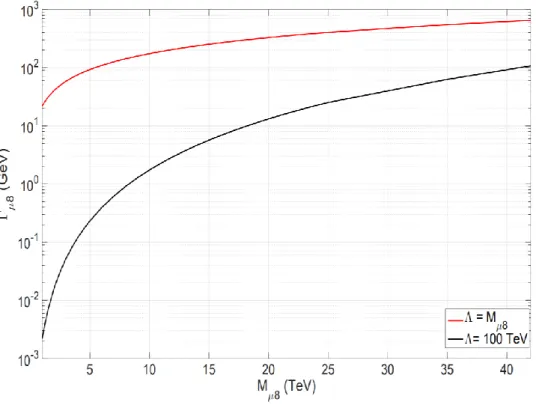
Γ_𝜇₈ = 𝛼𝑠𝑀𝜇8

3 4Λ2

As it can be understood from the expression, the decay width is directly proportional to the cube of the mass of 𝜇8, while it is inversely proportional to the square of the composite scale. Figure 4.1 shows the graph of the mass of 𝜇₈ against decay width. It should be stated here that when the color octet of the compositeness scale exceeds the mass of the muon, the decay width decreases approximately 10000 times. This value is approximately 10 times in 20 TeV 𝜇₈ mass.

(54)

32

Figure 4.1 Graph of decay width against the mass of 𝜇₈ at different compositeness scale

In this section, a comparative review of the color octet muon in various colliders will be made.

4.1 Resonant Production

The resonant production of color octet muons was investigated by the HEP group in TOBB ETU in order to determine the discovery potential of the FCC-based µp colliders [49]. In this study, the process was examined and the results of numerical calculations for this process are presented. Feynman diagram related to the resonant production of color octet muon is represented in Figure 4.2.

(55)

33

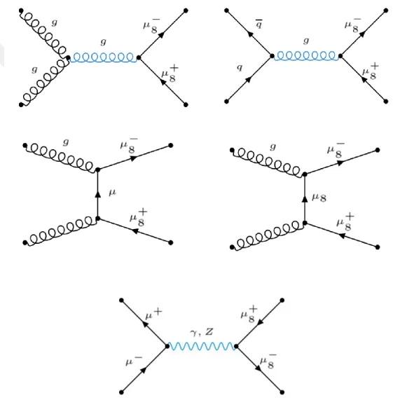
center-of-mass energy. Therefore, pair production of color octet muon has been investigated in hadron colliders [50]. From the results of the search of leptoquarks of the second family in ATLAS and CMS experiments, the mass of color octet muon should be more than 1.5 TeV. Figure 4.3 shows the Feynman diagrams of pair production in proton-proton colliders of 𝜇₈.

(56)

34 4.3 Indirect Production

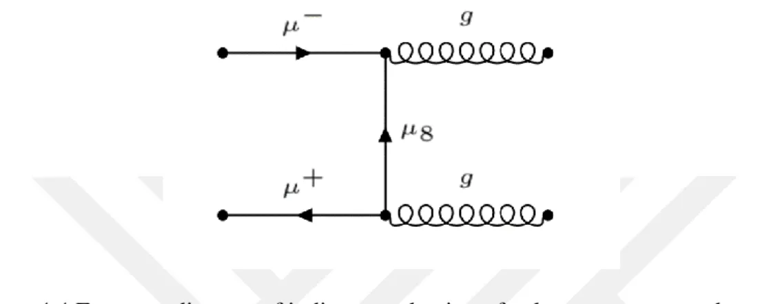
Only muon colliders have been studied in the indirect production of color octet muon. In this section, indirect production of the color octet muon in future muon colliders is examined and the potential of these colliders to investigate the color octet muon is determined. The signal process is 𝜇−_𝜇+ _{→ 𝑔𝑔 with 𝜇}

8 change in the t channel. The Feynman diagram of the procedure is shown in Figure 4.4.

Figure 4.4 Feynman diagram of indirect production of color octet muon at the muon colliders

The total cross sections for color octet muon at colliders with the center of mass energy is equal to 3 TeV, 6 TeV, 14 TeV is represented in Figure 4.5.

Figure 4.5 Distributions of indirect production cross sections according to mass of color octet muon at the three different muon colliders

(57)

35

Figure 4.6 Distribution of indirect production cross sections according to mass of color octet muon at the muon colliders with √𝑠 = 100 TeV

In Muon colliders, the background process of indirect production of 𝜇₈ is the photon and Z, two final states jets (𝜇−𝜇+ → 𝛾, 𝑍 → 𝑗 𝑗). Here 𝑗 = 𝑢, 𝑢̅, 𝑑, 𝑑̅, 𝑐, 𝑐̅, 𝑠, 𝑠̅, 𝑏, 𝑏̅. In Table 4.1, the center of mass energies and 1-year total luminosity values of the muon colliders we used in this study, are given. The distributions of transverse momentum (PT) and pseudo-rapidity (η) of the jets of the signal and background processes are given in Figures 4.6-4.15 to calculate the appropriate cuts in the muon colliders in this study.

Table 4.1 The values of 1-year integrated luminosity for the muon colliders with different center-of-mass energies

Colliders with √𝑠 Luminosity ( fb-1)

1.5 TeV 125 3 TeV 440 6 TeV 1200 14 TeV 1000 100 TeV 1000 1.00E-07 1.00E-06 1.00E-05 1.00E-04 1.00E-03 1.00E-02 1.00E-01 0 50000 100000 150000 200000 Cr o ss S e ction ( p b ) M_µ8(GeV)

(58)

36

Figure 4.7 Dispersions of transverse momentum for final state jets at muon collider with √𝑠 = 1.5 TeV.

Figure 4.8 Pseudo-rapidity dispersions of final state jets at muon collider with √𝑠 = 1.5 TeV.

(59)

37

Figure 4.9 Dispersions of transverse momentum for final state jets at muon collider with √𝑠 = 3 TeV.

Figure 4.10 Pseudo-rapidity dispersions of final state jets at muon collider with √𝑠 = 3 TeV.

(60)

38

(61)

39

(62)

40

(63)

41

Table 4.2 Transverse momentum and Pseudo-rapidity cuts for muon colliders

Colliders (TeV)

𝑷

_𝑻

(GeV)

𝜼

1.5

625 |𝜂| < 0.75

3 1250

|𝜂| < 0.75

6 2500

|𝜂| < 0.75

14 5800

|𝜂| < 0.75

100 41500

|𝜂| < 0.75

The following formula is used to calculate statistical significance. 𝑆 = 𝜎𝑠

√𝜎𝑠+ 𝜎𝑏 √𝐿𝑖𝑛𝑡

Here, 𝜎𝑠 and 𝜎𝑏 denote the cross-section values of signal and background, respectively. And Lint is integrated luminosity. In Figures 4.16, 4.17, 4.18, 4.19, and 4.20, the integrated luminosities required for the exclusion (2σ), observation (3σ), and (indirect) discovery (5σ) of the color octet muons at muon colliders with the center of mass energies, 1.5 TeV, 3 TeV, 6 TeV, 14 TeV, and 100 TeV, respectively. In these figures, the integrated luminosity is given depending on the mass of the color octet muon.

(64)

42

Figure 4.17 The required integrated luminosity for the indirect exclusion, observation, and discovery of 𝜇₈ for muon collider with √𝑠 = 1.5 TeV

Figure 4.18 The required integrated luminosity for the indirect exclusion, observation, and discovery of 𝜇₈ for muon collider with √𝑠 = 3 TeV

(65)

43

Figure 4.19 The required integrated luminosity for the indirect exclusion, observation, and discovery of 𝜇₈ for muon collider with √𝑠 = 6 TeV

Figure 4.20 The required integrated luminosity for the indirect exclusion, observation, and discovery of 𝜇8 for muon collider with √𝑠 = 14 TeV

(66)

44

Figure 4.21 The required integrated luminosity for the indirect exclusion, observation, and discovery of 𝜇₈ for muon collider with √𝑠 = 100 TeV The reachable mass values of color octet muon are given in Table 4.3 in the case of one and ten years of working at nominal luminosity.

Table 4.3 Accessible mass values of color octet muon for indirect exclusion, observation, and discovery at different colliders.

Colliders With √𝐬𝝁𝝁

years 𝟓𝝈 𝟑𝝈 𝟐𝝈

1.5 TeV

1 year 2740 GeV 2935 GeV 3095 GeV

10 year 3410 GeV 3190 GeV 3590 GeV

3 TeV

1 year 5345 GeV 5720 GeV 6035 GeV

10 year 6230 GeV 6655 GeV 7010 GeV

6 TeV

1 year 10250 GeV 10975 GeV 11600 GeV

(67)

45

10 year 24160 GeV 25880 GeV 27300 GeV

100 TeV

1 year 101000 GeV 111600 GeV 119800 GeV 10 year 124500 GeV 134800 GeV 143100 GeV

In the analysis up to this point, the compositeness scale is taken equal to the mass of color octet muon.

(68)

(69)

47

Although the Standard Model (SM) is a good model tested by experiments, it is considered to be a manifestation of a more basic model/theory due to the excess of the basic parameter and the number of particles it has. The historical process in revealing the most basic structure in progress supports this. In this thesis, preon models that predict that SM particles are composed of more basic building blocks are emphasized. The search for color octet muon, which is one of the particles predicted by Preon models, is researched in the colliders that are planned to be installed in the future. In the context of the research beyond SM, this study is important for examining the color octet muons in different colliders. Table 5.1 gives discovery mass limits on the search of μ₈ with the luminosity collected in different colliders in a year.

Table 5.1 Discovery mass limits on searching for μ₈ in different colliders

Colliders with √𝐬𝝁𝝁

years L (fb-1₎ _𝟓𝝈

1.5 TeV 1 year 125 2740 GeV

3 TeV 1 year 440 5345 GeV

6 TeV 1 year 1200 10250 GeV

14 TeV 1 year 1000 20570 GeV

100 TeV 1 year 1000 101000 GeV

It is shown that manifestations of color octet muons with masses up to 2.74 TeV, 5.35 TeV, 10.25 TeV, 20.57 TeV, and 101 TeV can be discovered at muon colliders with √s𝜇𝜇 equal to 1.5 TeV, 3 teV, 6 TeV, 14 TeV and 100 TeV, respectively.

(70)

48

(71)

49 REFERENCES

[1] Kaya, U., Oner, B. B., Sultansoy, S. (2018). A Minimal Fermiyon-Scalar Preonic Model. Turk J Phys, 42:235-241.

[2] Pati, J.C., and Salam, A. (1974). Lepton number as the fourth "color". Phys. Rev. D 10, 275- 289.

[3] Harari, H. (1979) A schematic model of quarks and leptons. Phys. Lett. B 86, 83-86.

[4] Fritzsch, H., Mandelbaum G. (1981). Weak interactions as manifestations of the substructure of leptons and quarks. Phys. Lett. B 102, 319-322.

[5] Greenberg, O.W., Sucher, J. (1981). A quantum structure dynamic model of quarks, leptons, weak vector bosons and Higgs mesons. Phys. Lett. B 99, 339-343.

[6] Barbieri, R., Mohapatra, R.N., Maseiro A. (1981). Compositeness and a left-right symmetric electroweak model without broken gauge interactions. Phys. Lett. B 105, 369-371.

[7] Baur, U., Streng K.H. (1985). Colored lepton mass bounds from pp collider data. Phys. Lett. B 162, 387-391.

[8] Celikel, A., Kantar, M., Sultansoy S. (1998). A search for sextet quarks and leptogluons at the LHC. Phys. Lett. B 443, 359-364.

[9] D’ Souza, I.A., Kalman, C.S. (1992). PREONS: Models of leptons, quarks and gauge bosons as composite objects. World Scientific, 1992.

[10] Shupe, M. A. (1979). A Composite Model of Leptons and Quarks. Phys. Lett. B 86, 87- 92.

[11] Harari, H., and Seiberg, N. (1982). The rishon model. Nuclear Physics B, 204, 141-167.

(72)

50

[12] Elbaz, E. (1986). Quark and lepton generation in the geometrical rishon model. Phys. Rev. D34, 1612-1618.

[13] Dugne, J. J., Fredriksson, S., Hansson, J., Predazzi, E. (1999). Preon trinity: A New model of leptons and quarks. Proceedings, 2nd International Conference on particle physics beyond the standard model, (Tegernsee, Germany, June 6-12), p. 285-296.

[14] Fariborz, A. H., Jora, R., Nasri, S. (2018). Mass Ansatze for the standard model fermions from a composite perspective. Rom.Rep.Phys. 70 (2018) 301. [15] Sahin, M., Sultansoy, S., Turkoz, S. (2010). Resonant Production of Color Octet

Electron at the LHeC, Phys. Lett. B689, 172-176.

[16] Akay, A. N., Karadeniz, H., Sahin, M. and Sultansoy, S. (2011). Indirect search of color octet electron at next generation linear colliders. Europhys. Lett. 95,31001.

[17] Liu, Z. L., Li, C. S., Wang, Y., Zhan, Y. C., Li, H. T. (2014). Transverse momentum resummation for color sextet and antitriplet scalar production at the LHC. Eur. Phys. J. C74 2771.

[18] Kohda, M., Sugiyama, H., Tsumura, K. (2013). Lepton number violation at the LHC with leptoquark and diquark. Phys.Lett. B718 1436-1440.

[19] Karabacak, D., Nandi, S., Rai, S. K. (2012). Diquark resonance and single top production at the Large Hadron Collider. Phys.Rev. D85 075011. [20] Richardson, P., Winn, D. (2012). Simulation of Sextet Diquark Production.

Eur.Phys.J. C72 1862.

[21] Han, T., Lewis, I., Liu, Z. (2010). Colored Resonant Signals at the LHC: Largest Rate and Simplest Topology. JHEP 1012 085.

[22] Enkhbat, T. (2014), Scalar leptoquarks and Higgs pair production at the LHC. JHEP 1401 158.

[23] Gonçalvez -Netto, D Lóp z-Val, D., Mawatari, K., Wigmore, I., Plehn T. (2013). Looking for leptogluons. Phys. Rew. D 87, 094023.

[24] Mandal, T. ve Mitra, S. (2013). Probing Color Octet Electrons at the LHC, Phys. Rev. D87 9, 095008.

(73)

51 April 2020)

[27] Anonymous. (2019d). https://home.cern/science/experiments/cms. (accessed in April 2020)

[28] Anonymous. (2019). https://home.cern/science/experiments/alice. (accessed in April 2020)

[29] Anonymous. (2018b). https://home.cern/science/experiments/lhcb. (accessed in April 2020)

[30] Anonymous. (2018). https://home.cern/topics/large-hadron-collider. (accessed in April 2020)

[31] Anonymous. (2018c). https://home.cern/science/experiments/lhcf. (accessed in April 2020)

[32] Anonymous. (2019e). https://home.cern/science/experiments/moedal. (accessed in April 2020)

[33] Anonymous. (2018a). https://home.cern/about/accelerators. (accessed in April 2020)

[34] Anonymous. (2019c). https://cds.cern.ch/record/2197559 (accessed at April 2020)

[35] Abada, A. et al. FCC Collaboration. (2018). Future Circular Collider: Vol. 1 Physics Opportunities. CERN-ACC-2018-0056.

[36] Abada, A. et al. FCC Collaboration. (2018). Future Circular Collider: Vol. 2 The Lepton Collider (FCC-ee). CERN-ACC-2018-0057.

[37] Abada, A. et al. FCC Collaboration. Future Circular Collider: Vol. 3 The Hadron Collider (FCC-hh). CERN-ACC-2018-0058.

[38] CEPC-SPPC, Preliminary Conceptual Design Report, IHEP-CEPC-DR-2015-01.