ISTANBUL KULTUR UNIVERSITY
INSTITUTE OF SCIENCES AND ENGINEERING
INTEGRATION OF GPS AND GIS
M.Sc. THESIS BY
HAMZA A. KHALEFA ABDALLA
A THESIS
SUBMITTED TO THE INSTITUTE OF SCIENCES AND ENGINEERING IN PARTIAL FULFILLMENT OF THE REQUIREMENTS
FOR THE DEGREE OF MASTER OF SCIENCE
Department : Civil Engineering
Program : Geomatics Engineering
Supervisor : Prof. Dr. Kamil EREN
ISTANBUL KULTUR UNIVERSITY
INSTITUTE OF SCIENCES AND ENGINEERING
INTEGRATION OF GPS AND GIS
M.Sc. THESIS BY
HAMZA A. KHALEFA ABDALLA
Civil Engineer
0209010001
Date of submission :
Date of defense examination :
Supervisor
: Prof. Dr. Kamil EREN
Members of Examining Committee : Prof. Dr. Turgut UZEL
Asst. Prof. Dr. Gürsel GÜZEL
ABSTRACT
Integration of GPS and GIS
Two of most exciting and effective technical developments to emerge in the last tow decade are: the Global Positioning System (GPS) and the Geographic Information System (GIS).
GPS is a powerful tool providing a unique position of a specific feature. It allows you to know where you are by consulting a radio receiver. The accuracies range as good as a few millimeters to somewhere around 100 meters, depending on equipment and procedures applied to the process of data collection.
While GIS is an extremely broad and complex field, concerned with the use of computers to input, store, retrieve, analyze, and display geographic information. Basically GIS programs make a computer think it’s a map, a map with wonderful powers to process spatial information, and to tell its users about any part of the world, at almost any level of detail.
Combining the GPS data with GIS allow for greater capabilities than what GPS and GIS can provide individually. With the combination of two technologies one is able to display the “Field/Actual Site” on a PC and make information decisions. There is no need to make specific site visits or review several documents/drawings. Also, anther benefit of the integration is the fact that the data can be shared by unlimited users in various departments for their own specific needs and analysis.
This work has two main objectives; the first objective is to study the integration of GPS and GIS technologies. The second objective is to design and establish a good and up-to-date base for a modern cadastre system for Beyşehir municipality, Turkey, by using the GPS and GIS techniques and other modern surveying instruments.
Table of Contents
Page No.
List of Tables... viii
List of Figures... ix List of Abbreviations... xi Acknowledgements... xiv 1.0 Introduction... 1 2.0 Background... 4
2.1 Global Positioning Sysem(GPS)... 4
2.1.1 GPS Concept... 4 2.1.2 Historical background... 5 2.1.3 GPS Segments... 6 2.1.3.1 Space segment... 6 2.1.3.2 Control segment... 10 2.1.3.3 User segment... 10 2.1.4 GPS signals... 11 2.1.4.1 Signal structure... 11 2.1.4.2 Pseudorange measurements... 12
2.1.4.3 Carrier phase measurements... 13
2.1.4.4 Signal processing... 14
2.1.5 GPS positioning modes... 15
2.1.5.1 Absolute point positioning... 15
2.1.5.2 Differential positioning... 15
2.1.5.3 Accuracy versus positioning mode... 16
2.1.6 GPS time system... 17
2.1.7 Height systems (Orthometric elevation)... 18
2.1.8 GPS receivers... 19
2.1.8.1 Receiver design... 19
2.1.8.2 Types of GPS receivers... 19
2.1.9.1 Orbital errors... 21
2.1.9.2 Satellites clock errors ... 21
2.1.9.3 Receiver clok errors... 22
2.1.9.4 Ionospheric errors... 22
2.1.9.5 Tropospheric errors... 23
2.1.9.6 Multipath errors... 24
2.1.9.7 Receiver noise... 25
2.1.9.8 SA and Anti-Spoofing (A-S)... 25
2.1.9.9 Setup errors... 26
2.1.9.10 Dilution of Precision (DOP)... 26
2.1.10 Planning a GPS survey... 28
2.1.11 GPS Error budget... 29
2.1.12 Common Data Exchange formats... 29
2.1.12.1 RINEX format... 30
2.1.12.2 Real time data transmission formats... 30
2.2 Geographic Information System (GIS)... 32
2.2.1 Historical review... 32
2.2.2 GIS definition... 35
2.2.3 Sources for GIS data... 37
2.2.4 Hardware components... 38
2.2.4.1 Input devices... 38
2.2.4.2 Processing and storage devices... 39
2.2.4.3 Output devices... 40 2.2.5 Software components... 41 2.2.5.1 Operating systems... 41 2.2.5.2 Programming languages... 41 2.2.5.3 Netwoking software... 41 2.2.5.4 Craphic standards... 42
2.2.6 Spatial data models... 42
2.2.6.1 Vector model... 42
2.2.6.2 Raster model... 43
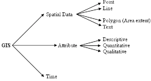
2.2.7 Geographic Data (Graphical & Attribute)... 44
2.2.8 GIS Datebase... 46
2.2.8.2 Logical Database design... 46
2.2.8.3 Physical Database design... 46
2.2.8.4 Database Implementation... 46 2.2.9 GIS systems... 47 2.2.10 Georeferencing... 48 2.2.10.1 Datum... 48 2.2.10.2 Coordinate systems... 50 2.2.10.3 Map projection... 52
2.3 GPS and GIS Integration... 57
2.3.1 GPS / GIS Integration Techniques... 57
2.3.1.1 Data-focused integration... 57
2.3.1.2 Position-focused integration... 58
2.3.1.3 Technology-focused integration... 60
3. Case Study Methodology and Equipments... 63
3.1 Methodology of the case study... 63
3.2 GIS technology used... 65
3.2.1 NetCAD 4.0 GIS... 65
3.2.2 Geographic referencing... 65
3.2.2.1 International Terrestrial Reference Frame 1996 (ITRF-96)... 66
3.2.2.2 Geodetic Reference System 1980(GRS80)... 66
3.2.2.3 European Datum 1950 (ED50)... 66
3.3 GPS Positioning Methods... 67
3.3.1 Static Positioning... 67
3.3.2 Real Time Kinematic (RTK) Positioning... 68
3.4 GPS equipments... 68
3.4.1 Magellan SporTrak GPS receiver... 68
3.4.2 Topcon HiPer GPS receiver... 69
3.4.3 Ashtech software... 71
3.5 Modern surveying instruments... 71
3.5.1 Topcon GTS-225 Total station... 71
4. case study... 74
4.1 Introduction... 74
4.1.1 Objective of the case study... 74
4.1.2 study area... 74
4.2 Exsiting maps and Data provided by General directorate of land registry and cadastrre... 76
4.2.1 Photogrammetric maps... 76
4.2.2 Turkish national fundamental GPS network (TUTGA)... 77
4.2.3 Turkish National Vertical Control Network (TUDKA)... 79
4.3 Scanning and digitizing... 79
4.3.1 Scanning... 80
4.3.2 Registration... 81
4.3.3 On-screen digitizing... 81
4.4 Work area boundaries (Village or quarter boundary)... 82
4.5 Geodetic Work (Geodetic control network)... 84
4.5.1 Network design in office... 84
4.5.2 Establish preliminary geodetic control network... 86
4.5.3 Final network points coordinates... 88
4.6 Data collection... 91 4.6.1 Field survey... 91 4.6.1.1 RTK GPS... 91 4.6.1.2 Total station... 93 4.6.1.3 Digital level... 96 4.6.2 Attribute Data... 96
4.7 Update (new maps)... 97
4.8 Data Base Management ... 98
4.8.1 Linking spatial and attribute data... 98
5. Conclusion... 100
References... 102
List of Tables
Page No.
Table 2.1 Satellite constellation status report (31 May 2005)... 8
Table 2.2 Error budget for absolute and relative GPS observations... 29
Table 2.3 Sample RINEX data file... 30
Table 2.4 Spatial data & Attributes... 45
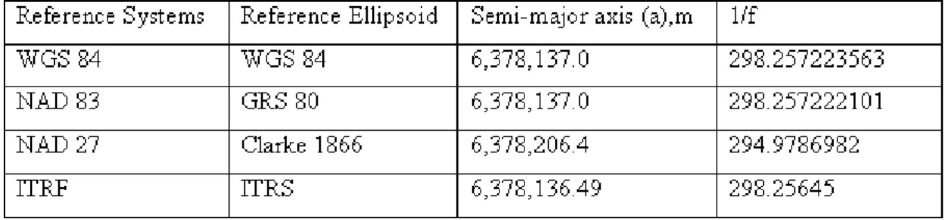
Table 2.5 Examples of reference systems and associated ellipsoids... 49
Table 3.1 Topcon HiPer GPS receiver accuracy... 70
Table 4.1 Details of study area... 75
Table 4.2 TUTGA points coordinates in work area... 78
Table 4.3 Sample of village boundary coordinates collected by handheld GPS.. 83
Table 4.4 Average distance between geodetic network points... 85
Table 4.5 Preliminary coordinates of GPS geodetic network... 87
Table 4.6 Geodetic network coordinates adjustment... 88
Table 4.7 Sample of coordinates collected by RTK GPS... 92
Table 4.8 Sample of data collected by total station... 94
List of Figures
Page No.
Figure 2.1 A & B, GPS satellites Constellation and planer projection... 7
Figure 2.2 Current structure of the GPS L1 and L2 satellite signals... 11
Figure 2.3 Principle of signal processing... 14
Figure 2.4 Differential or relative GPS positioning... 16
Figure 2.5 GPS accuracy and positioning modes... 17
Figure 2.6 Geoid and Ellipsoid relationship... 18
Figure 2.7 Basic concept of a receiver unit... 19
Figure 2.8 Multipath signals impacting GPS observations... 24
Figure 2.9 Satellite geometry and good & poor configurations... 27
Figure2.10 Sample of satellite availability and geometry... 28
Figure 2.11 GPS fix data (NMEA 0183 format)... 31
Figure 2.12 Interrelationship between GIS discipline... 32
Figure 2.13 Illustration of thematic layers... 33
Figure 2.14 Classical and Modern Geospatial Information System ... 35
Figure 2.15 Concept of a Geographic Information System... 36
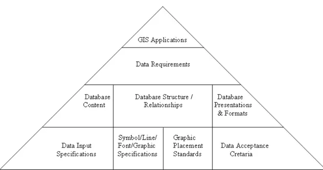
Figure 2.16 The basic five steps associated with GIS applications... 37
Figure 2.17 Hardware Components... 38
Figure 2.18 CPU and Main Computer Memory... 40
Figure 2.19 GIS basic components... 44
Figure 2.20 Top-down Datadase Design... 47
Figure 2.21 (a) Relationship between earth’s surface, geoid, and ellipsoid; and (b) ellipsoid parameters……….. 49
Figure 2.22 Geodetic and Cartesian coordinates... 51
Figure 2.23 The Universal transverse Mercator coordinate system ... 52
Figure 2.24 Universal Transverse Mercator (UTM) system... 54
Figure 2.25 Simple Cylindrical projections and UTM zone 14... 55
Figure 2.26 (a) Conic projection, and (b) Azimuthal projection... 56
Figure 2.27 Conceptual view of data-focused integration... 58
Figure 2.28 Conceptual representation of position-focused integration using two using two field device... 59
Figure 2.29 Conceptual representation of position-focused integration
using a single field device... 60
Figure 2.30 Conceptual representation of technology-focused integration... 61
Figure 3.1 Methodology of the case study... 64
Figure 3.2 Magellan SporTrak GPS receiver... 69
Figure 3.3 Topcon HiPer GPS receiver base and rove... 70
Figure 3.4 Topcon GTS-225 Total station (Topcon)... 72
Figure 3.5 Topcon DL-102 digital level ( Topcon)... 72
Figure 4.1 Map of turkey (Tapu Kadastro)... 75
Figure 4.2 Beyşehir city satellite image (Seydişehir kadastro)……….. 76
Figure 4.3 Sample of photogrammetric map (sheet) for rural area... 77
Figure 4.4 Distribution of TUTGA stations (Harita genel komutanlığı)... 78
Figure 4.5 Turkish National Vertical Control Network-1999 (TUDKA-99)... 79
Figure 4.6 Sample of scanning the map (sheet) in NetCAD... 80
Figure 4.7 Georeferencing... 81
Figure 4.8 Sample of map digitized... 82
Figure 4.9 All work area boundaries... 83
Figure 4.10 Sample of village boundary (Dumanlı köyü)... 84
Figure 4.11 Preliminary network design over Beyşehir map... 85
Figure 4.12 Sample output text file coordinates... 86
Figure 4.13 Draw preliminary coordiinates location by NetCAD... 87
Figure 4.14 A & B final geodetic network... 89
Figure 4.15 Total number of control points and work area boundary... 90
Figure 4.16 NetCAD is used for drawing farms (parcels)... 92
Figure 4.17 Sample of sketch draw in field... 93
Figure 4.18 Data transfers from total station to PC... 94
Figure 4.19 Sample of map draw depending on total station data collection... 95
Figure 4.20 Sample of Polygon points location... 95
Figure 4.21 Digital level way in our work area... 96
Figure 4.22 Enter the attribute information into the form... 97
Figure 4.23 Sample of new map (map updated)... 98
List of Abbreviations
1-D One-dimensional
2-D Two-dimensional
3-D Three-dimensional
AFB Air Force Base
A-S Anti-Spoofing
C/A-code Coarse /Acquisition code (1.023 MHz)
CAD Computer Add Design
CCD Charge-Coupled Device
CLI Canada Land Inventory
CPU Central Processing Unit
CRT Cathode Ray Tube (screen)
CYMK Cyan, Magenta, Yellow, Black (color spaces)
DBMS Data Base Management System
DGPS Differential Global Positioning System
DoD Department of Defense
DOP Dilution of Precision
DoT Department of Transportation
ECEF Earth Centered Earth Fixed
ED50 European Datum 1950
EER Enhanced Entity-Relationship (Data modeling)
ER Entity-Relationship (Data modeling)
ESRI Environmental System Research Institute
ETA Estimated Time of Arrival
FOC Full Operational Capability
GDOP Geometric Dilution of Precision
GIS Geographic Information System
GKS Graphic Kernal System
GLONASS Global Navigation Satellite System
GNSS Global Navigation Satellite System
GPS Global Positioning System
GRS80 Geodetic Reference System of 1980
HDOP Horizontal Dilution of Precision
IAG International Associated of Geodesy
IERS International Terrestrial Rotation Service
IGS International GPS Services
IOC Initial Operational Capability
ISO International Standard Organization
ITRF International Terrestrial Reference Frame
ITRS International Terrestrial Reference System
IUGG International Union of Geodesy and Geophysics
JPEG Joint Photographic Experts Group
JPO Joint Program Office
LAN Local Area Network
LIS Land Information System
LLR Lunar Laser Ranging
LRF Laser Range Finders
MHz Megahertz
MS-DOS Microsoft Disk Operating System
NAD1927 North American Datum of 1927
NANU Notice: Advisory to Navigation Users
NASA National Aeronautic and Space Administration
NATO North Atlantic Treaty Organization
NAVSTAR Navigation System with Timing and Ranging
NIS Navigation Information Service
NMEA National Maritime Electronics Association
NNSS Navy Navigation Satellite System (or TRANSIT)
OCS Operational Control System
PC Personal Computer
P-code Precision code (10.23 MHz)
PDOP Position Dilution of Precision
PPM Parts Per Million
PRN Pseudorandom Noise
RAM Random Access Memory
RF Radio Frequency
RINEX Receiver INdependent EXchange (format)
RMS Root Mean Square
RTCM Radio Technical Commission for Maritime (Services)
RTK Real Time Kinematic
SA Selective Availability
SLR Satellite Laser Ranging
SPS Standard Positioning Service
SVN Space Vehicle Number
TCP/IP Transmission Control Protocol/Internal Protocol
TDOP Time Dilution of Precision
TIFF Tagged Image File Format
UHF Ultra High Frequency
U.S. United States
USCG U.S. Coast Guard
U.S.S.R. Union of Soviet Socialist Republics
UTC Universal Time Coordinated
UTM Universal Transverse Mercator
VDOP Vertical Dilution of Precision
VHF Very High Frequency
VLBI Very Long Baseline Interferometry
WAN Wide Area Network
WGS84 World Geodetic System of 1984
Y-code Encrypted P-code
ACKNOWLEDGEMENTS
I would like to express my deepest gratitude to Prof. Dr. Turgut UZEL for supporting me in my graduate study. His guidance and consultation have provided an invaluable experience that will help me in my career.
My sincere appreciation goes to my supervisor Prof. Dr. Kamil EREN for his guidance and encouragement during my graduate thesis. I wish to extend my thanks to Prof. Dr. Ali RIZA GÜNBAK and Dr. Gürsel GÜZEL, for their supports.
My special thanks to the Professors, graduate students and staff at Civil Engineering Department. I would like to thank my numerous friends who helped me throughout this academic study.
On a personal level, I would like to thank my brothers and sisters for their supported. I am eternally grateful to both my parents for all the support and encouragement they have given me. Without you none of what I have accomplished would have been possible. Thank you my mother and my father.
Chapter 1
Introduction
The twentieth century gave rise to a great many different technologies, including the computer, wireless and cellular communication services, remote sensing, satellite navigation systems (GPS) and the Internet. The power of the technological innovation is significantly enhanced when it is integrated with other technologies. One such integration seen recently is GPS/GIS integration. GPS/GIS are such an extremely important technology. It is no exaggeration to say that GPS/GIS are revolutionizing aspects of many fields (engineering, geology, urban planning, natural resources, archaeology, agriculture, management, environmental protection, business, and many, many others).
A Geographic Information System (GIS) is a computer based information system that enables capture, modeling, manipulation, retrieval, analysis, and presentation of geographically referenced data. Spatial referenced data is data that is identified according to its geographic location (features). Today’s GIS, which are fundamentally a marriage of database management systems with graphics capability, are designed to allow for changes in the processor of individuals and organizations and changes in the data. GIS has caused a revolution in the way we look at geographic and environmental data. Datasets are organized as layers to create a digital representation of an area. Each layer provides some information (sometimes contradictory) about the reality. A layer can be a surface model of the terrain, an aerial image, a street map, or a distribution of population for a given area. Depending upon the application, different layers are combined to provide a composite view. Collecting data and putting them together is just a means to an end, not an end in itself. Therefore, one can see that the focus is now changing towards utilizing this data more intelligently. A large and comprehensive geographic dataset contains a huge wealth of different relationships, both within and between different layers. This is where visualization plays a major role. It is the purpose of visualization to present
the data in such a way that relationships and structures contained therein are made apparent.
The Global Positioning System (GPS) is a space-based radio navigation system operated by the United States Federal Government. The technology has been in existence for more than 20 years, and has been used by the U. S. Military and Air Force, but was not of much use at first for civilian users as the accuracy available for civilian applications. The removal of accuracy restrictions on civil users and the innovation of real time carrier phase tracking has opened the doors for a large variety of GPS applications. Given a favorable environment and certain settings it has now become possible to determine three-dimensional position with sub-meter accuracy. There has been a great increase in the number of GPS receiver manufacturers as well as companies devising GPS applications.
Spatial,or geographic, data can obtain from a variety of sources such as existing maps, satellite imagery, and GPS. Once the information collected, a GIS stores it as a collection of layers in the GIS database. The GIS can then be used to analyze the information and decisions can be made efficiently. For example, the decision to build a new road can be made by studying the effect of one feature such as traffic volume. GPS is used to collect the GIS field data efficiently and accurately. With GPS, the data is collected in a digital format in either real time or post-processed mode. A number of GPS/GIS systems that provide centimeter to meter level accuracy are now available on the market. Most of these systems allow the user to enter user defined attributes for each feature.
The growth in GIS is assured because it has been estimated that as much as 80% of all information used by governments and privates are referenced geographically. GIS is a tool that encourages planners, designers, and other decision-makers to study and analyze spatial data along with an enormous amount of attribute data (cultural, social, geographic, economic, resources, environmental, infrastructure, etc.) data that can be tagged to spatial entities.
This project has two main objectives. The first objective is to create a digital cadastral database for rural area in Beyşehir municipality in Turkey, that is tied to the
surface of the earth by coordinates, addresses, or other means are collectively called geospatial data. The second objective is to produce maps at different scale ranges for different proposes.
The thesis is organized into five chapters including this introductory chapter.
In the second chapter, necessity for background information and divided to three parts Global positioning system (GPS), Geographic information system (GIS), and GPS/GIS integration.
The third chapter deals with the methodology of the case study and equipments used to produce this work.
The fourth chapter is a case study, the case study was performed with the aim of showing that the research was not only conceptual but in fact was real cadastral project (Beyşehir village’s cadastral project, Turkey).
The fifth chapter provides a conclusion and summary of the results found in the previous chapters of this work.
Chapter 2
Background
We begin by presenting a GPS concept and a brief historical background on the GPS followed by a description of the general principle behind the system. We then focus on different error sources with GPS. We then deal with some basic GIS concepts. These include datum, coordinate systems, and map projections. Finally, description of the integration of GPS and GIS.
2.1 Global positioning system (GPS). 2.1.1 GPS Concept.
The NAVSTAR Global Positioning System (GPS) is a passive, all weather, 24-hours global navigation system GNSS designed, financed, deployed, operated, and maintained by the U.S. Department of Defense (DoD). It consists of a nominal constellation of 24 satellites in high altitude orbits. GPS has also demonstrated a significant benefit to the civilian community, who are applying GPS to a rapidly expanding number of applications, (Johan, 2002).
● Relatively high positioning accuracy, from meters down to the millimeter level. ● Capability of determining velocity and time.
● No inter-station visibility is required for high precision positioning. ● Result are obtained with reference to a single, global datum.
● Signals are available to users anywhere on the earth : in the air, on the ground, or at sea.
● No user charges.
● An all weather system, available 24 hours a day.
2.1.2 Historical background.
History changed on October 4, 1957, a significant technological breakthrough occurred when the Soviet Union successfully launched Sputnik I. The world first artificial satellite was about the size of a basketball, weighted only 183 pounds, and took about 98 minutes to orbit the earth on its elliptical path. That launch ushered in new political, military, technological, and scientific developments. While the Sputnik launch was a single event it marked the start to the space age and the U. S. - U. S. S. R. space race. On November 3, 1957, Sputnik II was launched, carrying a much heavier payload, including a dog named Laika. On January 31, 1958 the tide changed, when the United States successfully launched Explorer I. The GPS is actually the result of the merging of two independent programs that were begun in the early 1960’s. The U.S. Navy’s TIMATION Program and the U. S. Air Force’s 621b Project. Another system similar in basic concept of the current GPS was the Navy Navigation Satellite System (NNSS), also called TRANSIT system, which was also developed in the 1960’s. Currently, the entire system in maintained by the U. S. Air Force NAVSTAR GPS Joint Program Office (JPO).
Department of Defense (DoD) initially designed the GPS for military use only, providing sea, air, and ground troops of the United States and members of North Atlantic Treaty Organization (NATO), multi-service type organization that was established in 1973, with unified high-precision, all weather, world wide, real-time positioning system. The first U. S. pronouncement regarding civil use of GPS came in 1983 following the downing of Korean Airlines Flight 007 after it strayed over territory belonging the Soviet Union. As a result of this incident, in 1984, President Reagan announced the Global Positioning System (GPS) would be made available for international civil use once the system became operational. In 1987, DoD formally, requested the Department of Transportation (DoT) to establish and provide an office to respond to civil user’s needs and to work closely with the DoD to ensure proper implementation of GPS for civil use. Two years later, the U. S. coast guard became the lead agency for this project. On December 8, 1993 the DoD and DoT formally declared Initial Operational Capability (IOC), meaning that the NAVSTAR GPS was capable of sustaining the Standard Positioning Service (SPS). On April 27, 1995, the U. S. Air Force space command formally declared GPS met the
requirements for Full Operational Capability (FOC), meaning that the constellation of 24 operational satellites has successfully completed testing for military capability. Mandated by Congress, GPS is freely used by both the military and civilian public for real time absolute positioning of ship, aircraft, and land vehicle, as well as highly precise differential point positioning and time transferring.
2.1.3 GPS Segments.
The NAVSTAR GPS consists of three distinct segments: the space segment (satellite which broadcast signals), the control segment steering the whole system (ground tracking and monitoring station), and the user segment including the many type of receivers.
2.1.3.1 Space segment. ● Constellation.
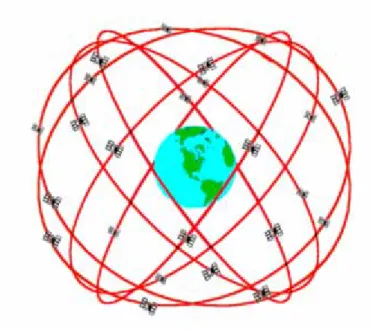
The GPS satellites have nearly circular orbital (an elliptical shape with a maximum eccentricity is about 0.01). The initial space segment was designed with four satellites in each of six orbits planes (A to F) with an inclination of about 55 degrees to the equator. The satellites are located at average altitudes of 20,200 km (10,900 nautical miles) above the earth’s surface and have 11-hours 58-minutes orbital periods, (Ahmed, 2002). The number of satellites in the GPS constellation has always been more than 24 operational satellites. With the full constellation, the space segment provides global coverage with four to eight simultaneously observable satellites above 15˚ elevation at any time of day. If the elevation mask is reduced to 10˚, occasionally up to 10 satellites will be visible; and if the elevation mask is further reduced to 5˚, occasionally 12 satellites will be visible, (Hofmann-Wellenhof, 2001).
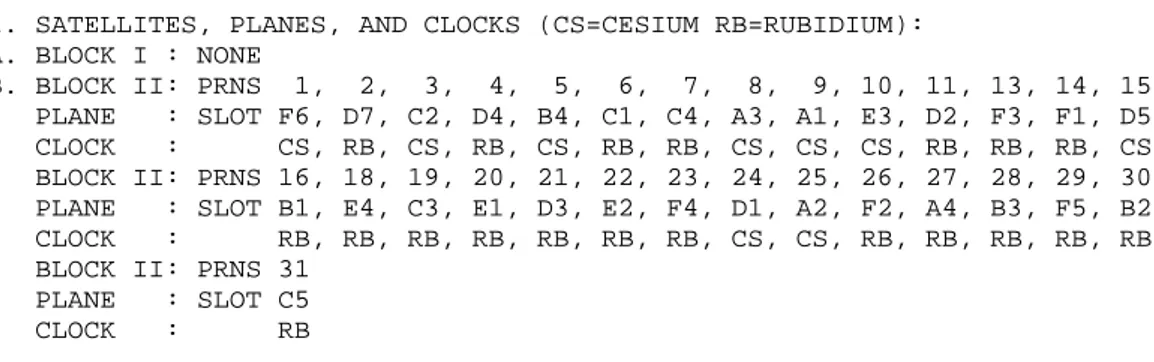
Current GPS satellite constellation : The current GPS satellite constellation (as of
31 May 2005) contain five Block II, 18 Block IIA, and six Block IIR satellites (Table 2.1 satellite constellation status report). This makers the total number of GPS
(a)
(b)
Figure 2.1 (a & b), GPS satellites Constellation and planer projection, (Peter, 2003). satellites in the constellation to be 29, which exceeds the nominal 24 satellites constellation by five satellites. All Block I satellites are no longer operational. As mention above, the GPS satellites are placed in six orbital planes, which are labeled
A through F. Since more satellites are currently available than the nominal 24-satellite constellation, an orbital plane may contain four, five, or six 24-satellites. As in table 2.1, the orbital plane A, B ,and E have four satellites, the orbital plane C has 5 satellites, and orbital planeD and F have six satellites.
Table 2.1 Satellite constellation status report (31 May 2005), (U. S. Coast Guard).
GPS OPERATIONAL ADVISORY 151 SUBJ: GPS STATUS 31 MAY 2005
1. SATELLITES, PLANES, AND CLOCKS (CS=CESIUM RB=RUBIDIUM): A. BLOCK I : NONE
B. BLOCK II: PRNS 1, 2, 3, 4, 5, 6, 7, 8, 9, 10, 11, 13, 14, 15 PLANE : SLOT F6, D7, C2, D4, B4, C1, C4, A3, A1, E3, D2, F3, F1, D5 CLOCK : CS, RB, CS, RB, CS, RB, RB, CS, CS, CS, RB, RB, RB, CS BLOCK II: PRNS 16, 18, 19, 20, 21, 22, 23, 24, 25, 26, 27, 28, 29, 30 PLANE : SLOT B1, E4, C3, E1, D3, E2, F4, D1, A2, F2, A4, B3, F5, B2 CLOCK : RB, RB, RB, RB, RB, RB, RB, CS, CS, RB, RB, RB, RB, RB BLOCK II: PRNS 31
PLANE : SLOT C5 CLOCK : RB
● Satellites.
The satellites have various systems of identification: launch sequence number, assigned pseudorandom noise (PRN) code, space vehicle number (SVN), orbital position number, NASA catalogue number, and international designation. (Hofmann-Wellenhof, 2001). The most popular identification systems within the GPS user community are the SVN and the PRN. Block II / IIA satellites are equipped with four onboard atomic clocks: two cesium (Cs) and two rubidium (Rb). The cesium clock is used as the primary timing source to control the GPS signal. Block IIR satellites, however, use rubidium clocks only, (Ahmed, 2002).
Satellite categories
There are six classes or types of GPS satellites. These are the Block I, Block II, Block IIA, Block IIR, Block IIF, and Block III satellites. GPS satellite constellation buildup started with a series of 11 satellites known as Block I satellites (weighting 845 kg). The first satellite in this series (and in the GPS system) was launched on February 22, 1978; the last was launched on October 9, 1985, from Vandenberg
AFB, California, with Atlas F launch vehicle. All launches were successful. The inclination angle of the orbital planes of these satellites, with respect to the equator, was 63˚. Although the design lifetime of Block I satellites were 4.5 years, some remained in service for more than 10 years. The last Block I satellite was taken out of service on November 18, 1995, (Ahmed, 2002). (Today none of the original Block I satellites are in operation).
The second generation of the GPS satellites is known as Block II satellites. The first Block II satellite, costing approximately $50 million and weighing more than 1500 kg, was launched on February 14, 1989, from the Kennedy space center, Cape Canaveral AFB in Florida, using a Delta II Rocket, (Hofmann-Wellenhof, 2001). The orbital plane of Block II satellites are inclined by 55 Degrees with respect to equator. The design lifetime of the Block II satellites is 7.5 years. Individual satellites, however, remained operated more than 10 years. The first Block IIA satellite (‘A’ denotes advanced) was launched on November 26, 1990. Block IIA is an advanced version of Block II, with an increase in the navigation message data storage capability from 14 days for Block II to 180 days for Block IIA satellites can function continuously, without ground support, for periods of 14 and 180 days respectively. A total of 28 Block II / IIA satellites were launched during the period from February 1989 to November 1997. Of these, 23 are currently in service. To ensure national security, some security features, known as Selective Availability (SA) and Anti-spoofing (A-S), were added to Block II/AII satellites. Today no distinction is made between Block II and Block IIA satellites, (Ahmed, 2002).
The Block IIR satellites (‘R’ denotes replenishment or replacement) weigh more than 2000 kg and the $ 42 million cost are about the same as for the Block II. The first Block IIR satellite was successfully launched on July 23, 1997 (Hofmann-Wellenhof, 2001). Block IIR consists of 21 satellites with a design life of 10 years. In addition to the expected higher accuracy, Block IIR satellites have the capability of operating autonomously for at least 180 days without ground corrections or accuracy degradation. The autonomous navigation capability of this satellite generation is achieved in part through mutual satellite ranging capabilities. In addition, predicted ephemeris and clock data for a period of 210 days are uploaded by the ground control
segment to support the autonomous navigation. As of May 2005, six Block IIR satellites have been successfully launched.
The Block IIF satellites (‘F’ denotes follow on) will weigh more than 2000 kg and the first Block IIF satellite is scheduled to be launched in 2005 or shortly after that date. Block IIF consisting of 33 satellites, the satellites life span will be 15 years. They will be equipped with improved on-board capabilities (such as internal navigation systems) and an augmented signal structure.
Presently, the DoD undertakes studies for the next generation of GPS satellites, called Block III satellites. These satellites are expected to carry GPS into 2030 and beyond, (Hofmann-Wellenhof, 2001).
2.1.3.2 Control segment.
The Operational Control System (OCS) consists of a master control station, six monitoring stations located throughout the worlds, and three ground control stations. The master Control Station is located at Schriever Air Force Base, Colorado with a backup station in Gaithersburg, Maryland. The information obtained from the monitoring stations that track the satellites is used in controlling the satellites and predicting their orbits. All data from the tracking stations are transmitted to the Master Control Station where it is processed and analyzed. Ephemeredes, clock corrections, and other message data are then transmitted back to the monitoring stations with ground antennas for subsequent transmittal back to the satellites. The Master Control Station is also responsible for the daily management and control of the GPS satellites and the overall control segment, (U.S. army, 2003).
2.1.3.3 User segment.
The user segment represents the ground based GPS receiver units that process the NAVSTAR satellite signals and compute the position and / or velocity of the user. Most GPS receivers perform these functions automatically, in real time, and often provide visual and/or verbal positional guidance information. Users consist of both
military and civil activities, for an almost unlimited number of applications in a variety of air, sea, or land based platforms.
2.1.4 GPS signals.
2.1.4.1 Signals structure.
Each NAVSTAR satellite transmits ranging signals on two L-band frequencies, designed as L1 and L2. The L1 carrier frequency is 1575.42 megahertz (MHz) and has a wavelength of approximately 19 cm. The L2carrier frequency is 1227.60 MHz and has a wavelength of approximately 24 cm. The L1 signal is modulated with a 1.023 MHz Coarse/Acquisition Code (C/A-code) and a 10.23 MHz Precision Code (P-code). The L2 signal is modulated with only the 10.23 MHz P-code. Both codes can be used to determine the range between the user and a satellite. The P-code is normally encrypted and is available only to authorized users. When encrypted, it is termed the Y-code, Figure 2.2 summarizes the carrier frequencies and codes. Each satellite carrier’s precise atomic clocks to generate the timing information needed for precise positioning. A 50 Hz navigation message is also transmitted on both the P(Y)-code and C/A-code. This message contains satellite clock bias data, satellite ephemeris data, orbital information, ionospheric signal propagation correction data, health and status of satellites, and satellites almanac data for the entire constellation.
2.1.4.2 Pseudorange Measurements.
Pseudorange observations are obtained by measuring the transit time of the signal as it travels from the GPS satellite to the receiving antenna. Due to non-synchronized receiver and satellite clocks, the measured range (pseudorange) is biased. Therefore, the receiver’s clock difference with respect to the satellite’s GPS time must be taken into account. This leads to a system of equations with four unknown parameters (three coordinates and clock drift); thus at least four satellite observations are necessary for position calculation.
The code observable P for a single satellite can be expressed as (Salytcheva, 2004): P = ρ + dρ + c(dt- dT) + dion +dtrop + εp
where: ρ is the geometric range between the GPS satellite and receiver antenna (m);
dρ is the orbital error (m); dt is the satellite clock error (s); dT is the receiver clock error (s); dion is the ionospheric delay (m); dtrop is the tropospheric delay (m);
εp is the code noise (receiver noise + multipath) (m); and c is the speed of electromagnetic wave in vacuum (m/s).
Orbital, satellite clock, and atmospheric errors can be reduced or even eliminated by differencing pseudorange measurements with a receiver at a known location (DGPS). The receiver clock error is usually included as an unknown parameter in single point and single difference GPS methods. Noise depends on the received signal strength and on the correlation method employed in the receiver, so that it cannot be decreased without access to the hardware. Multipath is caused by multiple reflections of GPS signals interfering with the line-of-sight signal (LOS). It is environmentally dependent and thus cannot be mitigated by DGPS. This error is also difficult to model and therefore to satisfactorily compensate.
2.1.4.3 Carrier phase measurements.
Carrier frequency tracking measures the phase differences between the Doppler shifted satellite and receiver frequencies. Phase measurements are resolved over the relatively short L1 and L2 carrier wavelengths (19 cm and 24cm respectively). This allows phase resolution at the mm level. The phase differences are continuously charging due to changing satellite earth geometry. However, such effects are resolved in the receiver and subsequent data post-processing. When carrier phase measurements are observed and compared between two stations (i.e. relative or differential mode), baseline vector accuracy between the stations below the centimeter level in attainable in three dimensions. Various receiver technologies and processing techniques allow carrier phase measurements to be used in real-time centimeter positioning.
The Doppler, in the case of GPS, is a measurement of the instantaneous phase rate of a tracked satellite’s signal; as a result, the velocity of the user with respect to the GPS satellites can be determined. Doppler measurements are also error-corrupted, (Salytcheva, 2004):
ф = ρ + dρ + c(dt- dT) - dion +dtrop + εφ
where: ф is the Doppler observable (m/s);
ρ is the geometric range rate (m/s);
dρ is the orbital error drift (m/s); dt is the satellite clock drift; dT is the receiver clock drift;
dion is the ionospheric delay drift (m/s); dtrop is the tropospheric delay drift (m/s);
ε
φ is the receiver noise and the rate of change of multipath (m/s). Similarly to pseudorange errors, the atmospheric effects and satellite clock drift are reduced by DGPS, where the receiver clock drift is considered in the velocity calculation scheme as an unknown parameter, so that a minimum of four Doppler observables is needed to solve for the user’s velocity.2.1.4.4 Signal processing.
The signal emitted from the satellite is represented by the equations (Hofmann-Wellenhof, 2001).
L1(t) = a1. P(t). W(t). D(t) cos (f1. t) + a1. C/A(t). D(t) sin (f1. t) L2(t) = a2. P(t). W(t). D(t) cos (f2. t)
Where : Li (t) = ai cos (fi. t) the unmodulated carriers.
P(t), C/A(t), W(t), and D(t) the state sequences of the P-code, the C/A-code, the W-code, and the
Navigation message respectively .
And contains three components in the symbolic form (L1, C/A, D), (L1, Y, D), and (L2, Y, D). The goal of signal processing by the GPS receiver is the recovery of the signal components, including the reconstruction of the carrier wave and the extraction of the codes for the satellite clock readings and the navigation message. (Hofmann-Wellenhof, 2001). The principle is illustrated in figure 2.3.
2.1.5 GPS positioning modes.
There are basically two general operating modes from which GPS-derived positions can be obtained: (1) absolute positioning, and (2) differential (or relative) positioning. Within each of these two modes, range measurements to the satellites can be performed by tracking either the phase of the satellite’s carrier signal or the pseudo-random noise (PRN) codes modulated on the carrier signal.
2.1.5.1 Absolute point positioning.
Absolute positioning involves the use of only a single passive receiver at the user’s location to collect data from multiple satellites in order to determine the user’s georeferenced position. GPS determination of a point position on the earth actually user a technique common to terrestrial surveying called trilateration (i.e., electronic distance measurement resection). The user’s GPS receiver simply measures the distance (range) between the earth and the NAVSTAR GPS satellites. The user’s position is determined by the resected intersection of the observed ranges to the satellites. In actual practice, at least 4 satellite observations are required in order to resolve timing variations. Adding more satellite ranges will provide redundancy (and more accuracy) in the position solution, (US Army, 2003).
2.1.5.2 Differential positioning.
Differential GPS positioning is simply a process of determining the relative differences in coordinates between two receiver points, each of which is simultaneously observing/measuring satellite code ranges and/or carrier phases from the NAVSTAR GPS satellite constellation. These differential observations, in fact, derive a differential baseline vector between the two points, as shown in figure 2.4. This method will position two stations relative to each other, hence the term relative positioning, and can provide the higher accuracies required for project. There are basically two general types of differential positioning:
● Code phase pseudorange tracking. ● Carrier phase tracking.
Both methods, either directly or indirectly, determine the distance, or range, between a NAVSTAR GPS satellite and a ground-based receiver antenna. These measurements are made simultaneously at two different receiver stations. Either the satellite’s carrier frequency phase, or the phase of a digital code modulated on the carrier phase, may be tracked depending on the type of receiver. Through various processing techniques, the distance between the satellites and receivers can be resolved, and the relative positions of the two receiver points are derived. From these relative observations, a baseline vector between the points is generated. The resultant accuracy is depending on the tracking method used carrier phase tracking being far more accurate than code phase tracking, (US Army, 2003).
Figure 2.4 Differential or relative GPS positioning, (US Army, 2003).
2.1.5.3 Accuracy versus positioning mode.
The different positioning associated with the different GPS positioning modes, as shown in figure 2.5, (accuracy is quoted as two-sigma values, i.e., 95% confidence level). In all cases, the vertical accuracy is about 2 times worse than the horizontal positioning accuracy. It should be emphasised that GPS was designed to provide accuracies of the order of a dekametre (ten meters) or so in the absolute positioning
mode, and is optimised for real-time operations. All other developments to improve this basic accuracy capability must be viewed in this context. As a general axiom of GPS positioning, the higher the accuracy sought, the more effort (in time, instrumentation and processing sophistication) is required, (John, 2001).
Figure 2.5 GPS Accuracy and positioning modes, (John, 2001).
2.1.6 GPS time system.
Time plays is a very important role in positioning with GPS, the GPS signal is controlled by accurate timing devices, the atomic satellite clock, measuring the ranges (distances) from the receiver to the satellites is based on both the receiver and the satellite clocks. GPS is also a timing system, that is, it can be used for time synchronization. A number of time systems are used worldwide for various purposes; they are based on various periodic processes such as Earth rotation. (Hofmann-Wellenhof, 2001). GPS time is accurately maintained and monitored by the DoD. GPS time is usually maintained within 30 nanoseconds of universal time coordinated (UTC). GPS time is based on a reference ‘GPS epoch’ of 000 hours (UTC) 6 January 1980, the relationship between GPS time and UTC is following, (US Army, 2003). GPS time = UTC + number of leap seconds + [GPS-to-UTC bias]
GPS receivers obtain time corrections from the broadcast data messages and can thus output UTC time increments.
2.1.7 Height systems ( Orthometric elevation).
Geoidal heights represent the geoid-ellipsoid separation distance measured along the ellipsoid normal and is obtained by taking the difference between ellipsoidal and orthometric height values. Knowledge of the geoid height enable the evaluation of vertical positions either the geodetic (ellipsoid based) or the orthometric height system. The relationship between a WGS84 ellipsoidal height and an orthometric height relative to the geoid can be obtained from the following equation, (US Army, 2003).
Һ = H + N Where:
һ = ellipsoidal height (WGS84).
H = elevation (orthometric–normal to geoid).
N = geoidal undulation above or below the WGS84 ellipsoid.
2.1.8 GPS receivers.
There is a variety of receivers on the market used for different purposes (navigation, surveying, time transfer) and with different features. Despite this variety, all the receivers employ certain common principles.
2.1.8.1 Receiver design.
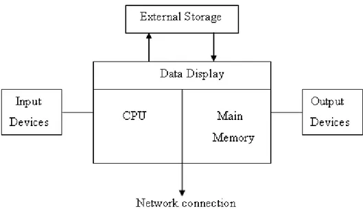
GPS receiver collects radio waves from various satellites, compares clock times, performs calculations, displays the results on a display device, and stores data in a file for later output. The components must receive, store, display, record, and output data. The receiver structure is shown in figure 2.7, It consist of an antenna, a Radio Frequency (RF) section, processor, control device, storage device, and power supply.
Figure 2.7 Basic concept of a receiver unit, (Hofmann-Wellenhof, 2001).
2.1.8.2 Types of GPS receivers.
In 1980, only one commercial GPS receiver was available on the market, at a price of several hundred thousand U.S. dollars. This, however, has changed considerably as more than 500 different GPS receivers are available in today’s market from 58 manufacturers. The current receiver price varies from about $ 200 for the simple handheld units to about $ 35000 for the sophisticated geodetic quality units. Commercial GPS receivers may be divided into four types, according to their receiving capabilities, (Ahmed, 2002). These are:
● The single frequency code receiver: It measures the pseudo-range with the C/A-code only. It is the least expensive and the least accurate receiver type and is mostly used for recreation purposes.
● The single frequency carrier smoothed code receivers: It is also measures the pseudo-ranges with the C/A-code only. The higher resolution carrier frequency is used internally to improve the resolution of the code pseudo-range, which results in high precision pseudo-range measurements.
● The single frequency code and carrier receivers: Output the raw C/A-code pseudo-range, the L1 carrier phase measurements, and the navigation message. In addition, this receiver type is capable of performing the functions of the other receiver types. ● The Dual frequency receivers: They are the most sophisticated and most expensive receiver type. Before the activation of AS, dual frequency receivers were capable of outputting all the GPS signal components (i.e., L1and L2 carriers, C/A-code, P-code on both L1and L2, and the navigation message). However, after the AS activation, the P-code was encrypted to Y-code. This means that the receiver cannot output either the P-code or the L2 carrier using the traditional signal recovering technique. To overcome this problem, GPS receiver manufacturers invented a number of techniques that do not require information of the Y-code. At the present time, most receivers use two techniques known as the Z-tracking and the cross-correlation techniques. Both techniques recover the full L2 carrier, but at a degraded signal strength. The amount of signal strength degradation is higher in the cross-correlation techniques compared with the Z-tracking technique.
GPS receivers can also be categorized according to their number of tracking channels, which varies from 1 to 12 channels. A good GPS receiver would be multi-channel, with each channel dedicated to continuously tracking a particular satellite. Presently, most GPS receivers have 9 to 12 independent (or parallel) channels. Features such as cost, ease of use, power consumption, size and weight, internal and/or external data storage capabilities, interfacing capabilities, and multi-path mitigation (i.e., type of correlator) are to be considered when selecting a GPS receiver.
2.1.9 GPS Errors. 2.1.9.1 Orbital Errors.
Orbital errors occur due to the differences in the actual and modeled positions of the satellites. Three sets of data are available to determine position and velocity vectors of the satellites in a terrestrial reference frame at any instant: almanac data, broadcast ephemerides, and precise ephemerides, (Hofmann-Wellenhof, 2001). Broadcast ephemeredes are available in real time and orbital parameters are uploaded for each interval of two hours. Currently, this type of satellite orbit has an RMS accuracy of about 3 m. More accurate orbit information of about 5 cm can be obtained from the International GPS Service (IGS); however, it is available only from a few days, up to a week, after the observations. Fortunately, orbital errors are correlated for two receivers simultaneously tracking the same satellite and thus can be diminished by differencing observations between the receivers. The remaining errors are generally in the range of much less than 0.5 parts per million (ppm). PPM is the measure of residual errors in GPS measurements, when differential GPS is used. One ppm means that one cm of position error is introduced per ten km baseline, (Salytcheva, 2004).
2.1.9.2 Satellite clock errors.
GPS satellites carry rubidium and cesium time standards that are usually accurate to 1 part in 1012 and 1 part in 1013, respectively. Rang error observed by the user as the
result of time offset between the satellite and receiver clock is a linear relationship and can be approximated by the following formula, (US Army, 2003).
RE = T0 * c
Where:
RE = range error due to clock instability. T0 = time offset.
c = speed of light.
T0 = 1 microsecond (μs) = 10−6 seconds.
c = 299,792,458 m/s. RE = (10
6
− s) * 299,792,458 m/s = 299.79 m = 300 m.
This means that one nanosecond error is equivalent to a range error of about 30 cm. the satellite clock error is about 8.64 to 17.28 ns per day. The corresponding range error is 2.59 m to 5.18 m, (Ahmed, 2002). The amount of drift is calculated and transmitted as a part of the navigation message in the form of three coefficients of a second-degree polynomial. This error can be eliminated by the DGPS.
2.1.9.3 Receiver clock error.
GPS receivers use inexpensive crystal clocks, which are much less accurate than the satellite clocks. This error can range from 200 ns up to a few ms, and changes over time due to the clock drift, (Salytcheva, 2004). It can be removed through differencing between the satellites or it can be treated as an additional unknown parameter in the estimation process.
2.1.9.4 Ionospheric errors.
The ionosphere, extending in various layers from about 50 km to 1000 km above earth, is a dispersive medium with respect to the GPS radio signal, (Hofmann-Wellenhof, 2001). The ionosphere is formed by ultraviolet and X-ray radiations coming from the sun interact with the gas modecules and atoms. These interactions result in gas ionization: a large number of free “negatively charged” electrons and “positively charged” atoms and moleculer, (Ahmed, 2002). The ionosphere bends the GPS radio signal and changes its speed as it passes through the various ionospheric layers to reach a GPS receiver.
The error of ionosphere refraction on the GPS range values is dependent on sunspot activity, time of day, and satellite geometry. Ionospheric delay can vary from 40-60 m during the day and 6-12 m at night. GPS operations conducted during periods of high sunspot activity or with satellites near the horizon produce range results with the most error. GPS operations conducted during periods of low sunspot activity, during
the night, or with a satellite near the zenith produce range results with the least amount of ionospheric error, (US Army, 2003).
Resolution of ionospheric refraction can be accomplished by use of a dual-frequency receiver. During a period of uninterrupted observation of L1and L2 signals, these signals can be continuously counted and differenced, and the ionospheric delay uncertainty can be reduced to less than 5 m. The resultant difference reflects the variable effects of the ionosphere delay on the GPS signal, (US Army, 2003).
2.1.9.5 Tropospheric errors.
The troposphere is the electrically neutral atmospheric region that extends up to about 50 km from the surface of the earth. The troposphere is a non-dispersive medium for radio frequencies below 15 GHz. As a result, it delays the GPS carriers and codes identically. The tropospheric delay depends on the temperature, pressure, and humidity along the signal path through the troposphere. Tropospheric delay results in values of about 2.3 m at zenith (satellite directly overhead), about 9.3 m for a 15˚ elevation angle, and about 20-28 m for a 5˚ elevation angle, (Ahmed, 2002). The tropospheric conditions causing refraction of the GPS signal can be modeled by measuring the dry and wet components. The dry component represents about 90% of the delay and can be predicted to a high degree of accuracy using mathematical models, (Ahmed, 2002). The dry component is best approximated by following equation, (US Army, 2003):
DC = (2.27 * 0.001) * P0
Where: Dc = dry term range contribution in zenith direction in meters. P0 = surface pressure in millibar (mb).
The average of atmospheric pressure is P0 = 1013.243 mb.
The wet component is considerably more difficult to approximate because its approximation is dependent not just on surface conditions, but also on the atmospheric conditions (water vapor content, temperature, altitude, and angle of the signal path above the horizon) along the entire GPS signal path. As this is the case, there has not been a well correlated model that approximates the wet component, (US Army, 2003).
2.1.9.6 Multipath errors.
This effect is well described by its name: a satellite-emitted signal arrives at the receiver via more than one path. Multipath is mainly caused by reflecting surfaces near the receiver. Secondary effects are reflections at the satellite during signal transmission, (Hofmann-Wellenhof, 2001). Referring to figure 2.8 the satellite signals arrives at the receiver on four different paths, two direct and two indirect.
Figure 2.8 Multipath signals impacting GPS observations, (US Army, 2003). The range errors caused by multipath will vary depending on the relative geometry of the satellites, reflecting surfaces and the GPS antenna, and also the properties and dynamics of the reflecting surfaces, (John, 2001). With the newer receiver and antenna designs, and sound prior mission planning to reduce the possible causes of multipath, the effects of multipath as an error source can be minimized. Averaging of GPS signals over a period of time (i.e., different satellite configurations) can also help to reduce the effects of multipath, (US Army, 2003).
2.1.9.7 Receiver noise.
Receiver noise includes a variety of errors associated with the ability of the GPS receiver to measure a finite time difference. These include signal processing, clock/signal synchronization and correlation methods, receiver resolution, signal noise, and others, (US Army, 2003).
The receiver measurement noise results from limitations of the receiver’s electronics. A good GPS system should have a minimum noise level. Two tests can be performed for evaluating a GPS receiver: zero baseline and short baseline tests. (Ahmed, 2001). A zero baseline test is used to evaluate the receiver performance. The test involves using one antenna/preamplifier followed by a signal splitter that feeds two or more GPS receivers. As one antenna is used, the baseline solution should be zero. In other words, any nonzero value is attributed to the receiver noise. Although the zero baseline test provides useful information on the receiver performance. The contribution of the receiver measurement noise to the range error will depend very much on the quality of the GPS receiver. Typical average value for range error due to the receiver measurement noise is of the order of 0.6 m (1σ-level), (Ahmed, 2001). To evaluate the actual field performance of a GPS system. This can be done using short baselines of a few meters apart, observed on two consecutive days. In this case, the double difference residuals of one day would contain the system noise and the multipath effect. All other errors would cancel sufficiently. As the multipath signature repeats every sidereal day, differencing the double difference residuals between the two consecutive days eliminates the effect of multipath and leaves only the system noise, (Ahmed, 2001).
2.1.9.8 Selective Availability (SA) and Anti-Spoofing (A-S).
Before May 2000, SA was activated to purposely degrade the satellite signal to create position errors. This is done by dithering the satellite clock and offsetting the satellite orbits, (US Army, 2003). To ensure national security, the U.S. DoD implemented SA on Block II GPS satellites to deny accurate real time autonomous
positioning to unauthorized users. SA was officially activated on March 25, 1990. With SA turned on, nominal horizontal and vertical errors can be up to 100 m and 156 m, respectively. SA was turned off on May 1, 2000, (Ahmed, 2001).
A-S is accomplished by the modulo 2 sum of the P-code and an encrypting W-code. The resulting code is denoted as the Y-code, (Hofmann-Wellenhof, 2001). A-S was implemented on 31 January, 1994, The rationale behind this decision was that by keeping the military PRN code secret.
2.1.9.9 Setup errors.
Centering errors can be reduced if the equipment is checked to ensure that the optical plummet is true. High measuring errors can be reduced by utilizing equipment that provides a built-in (or accessory) measuring capability to measure precisely (either directly or indirectly) the antenna height (hi) or by using fixed length tripods and bipods, (Barry, 2003).
2.1.9.10 Dilution of Precision (DOP).
The geometry of the visible satellites is an important factor in achieving high quality results especially for point positioning and kinematic surveying. The geometry changes with time due to the relative motion of the satellites. A measure of the geometry is the Dilution of Precision (DOP) factor, (Hofmann-Wellenhof, 2001). The lower the value of the DOP numbers, the better the geometric strength, and vice versa. Good satellite geometry is obtained when the satellites are spread out in the sky. In general, the more spread out the satellites are in the sky, the better the satellite geometry, and vice versa, as shown in figure 2.9. The Geometry dilution of precision (GDOP) is further classified so as to represent the accuracy of the components of Position and time. These are termed as Position Dilution of Precision (PDOP), Horizontal Dilution of Precision (HDOP), Vertical Dilution of Precision (VDOP), and Time Dilution of Precision (TDOP).
Figure 2.9 Satellite geometry and good & poor configurations, (US Army, 2003). GDOP is defined to be the square root of the sum of the variances of the position and time error estimates, (US Army, 2003).
GDOP = [σE 2 + σ N 2 + σU 2 + σR 2 + (c * δT)2]0.5. [1/σR] Where:
σE = standard deviation in east value, m. σN = standard deviation in north value, m. σU = standard deviation in up direction, m. c = speed of light (299,729,458 m/s). δT = standard deviation in time, seconds.
σR = overall standard deviation in range in meters, at the 1σ (68%) level. PDOP is a measure of the accuracy in 3-D position, mathematically defined as:
PDOP = [σE 2 +σ N 2 + σU 2]0.5. [1/σR]
HDOP is a measurement of the accuracy in 2-D horizontal position, mathematically defined as: HDOP = [σE 2 +σ N 2]0.5. [1/σ R]
VDOP is a measurement of the accuracy in standard deviation in vertical height, mathematically defined as:
VDOP = [σ U]* [1/σ R]
In general, GDOP and PDOP values should be less than 6 for a reliable solution. Optimally, they should be less than 5. GPS performance for HDOP is normally in the 2 to 3 range. VDOP is typically around 3 to 4. Increase above these values levels may indicate less accurate positioning. In most cases, VDOP values will closely resemble PDOP values. It is also desirable to have a GDOP/PDOP that changes during the time of GPS survey session. The lower the GDOP/PDOP, the better the instantaneous point position solution is, (US Army, 2003).
2.1.10 Planning a GPS survey.
Planning is important for GPS surveys so that almanac data can be analyzed to obtain optimal time to sets when a geometrically strong array of satellites is available above 15˚ of elevation (above the horizon) and to identify topographic obstructions that may hinder signal reception. Planning software can graphically display GDOP at each time of the day, as shown in figure 4. The surveyor can use Planning software to help the mission planning process and select not only the optimal days for the survey, but also the hours of the day that will result in the best data.
2.1.11 GPS Error budget.
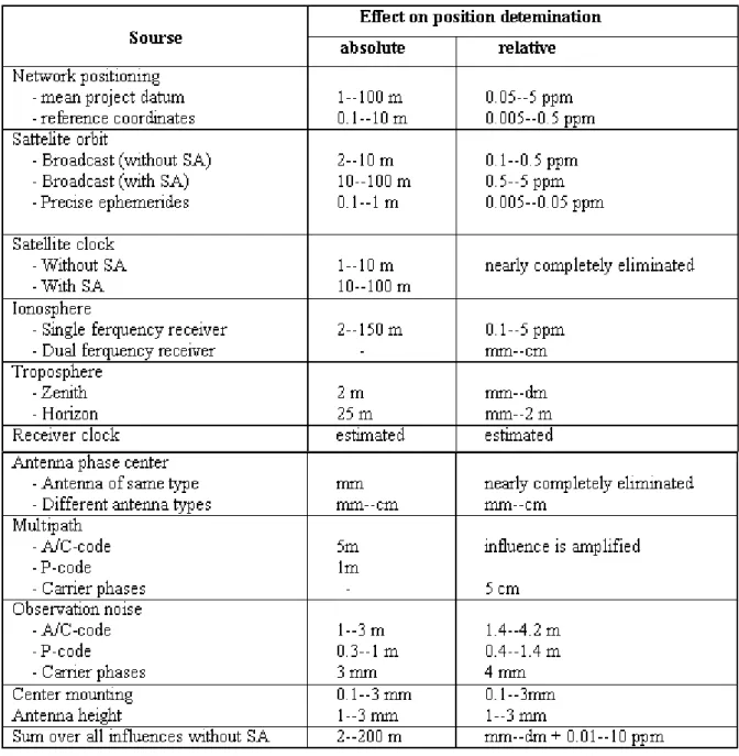
Table 2.2 gives an overview on the main error sources in GPS positioning.
Table 2.2 Error budget for absolute and relative GPS observations, (Günter, 2000).
2.1.12 Common Data Exchange formats.
Since individual GPS manufacturers have their own proprietary formats for storing GPS measurements, it can be difficult to combine data from different receivers. A similar problem is encountered when interfacing various devices including the GPS
system. To overcome these limitations, a number of research groups have developed standard formats for various user needs.
2.1.12.1 RINEX format.
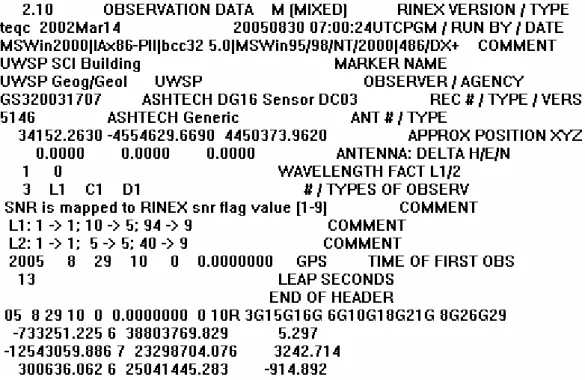
The Receiver INdependent EXchange (RINEX) format is an ASCII type format that allows a user to combine data from different manufacturer’s receivers, (US Army, 2003). The current RINEX version 2.10 defines six different RINEX files; each contains a header and data sections: (1) observation data file, (2) navigation message file, (3) meteorological file, (4) GLONASS navigation message file, (5) geostationary satellites (GPS signal payloads) data file, and (6) satellite and receiver clock data file. Table 2.3 shows sample RINEX V2.10 data file. For the majority of GPS users, the first three files are the most important. The record, or line, length of all RINEX files is restricted to a maximum of 80 characters, (Ahmed, 2001).
Table 2.3 Sample RINEX data file, (Advanced computer lab, 2005).
2.1.12.2 Real time data transmission formats.
There are two common types of data formats used most often during real time surveying. They are (1) RTCM SC-104 and (2) NMEA.
● Transmission of data between GPS receivers: The Radio Technical Commission for Maritime services (RTCM) is the governing body for transmissions used for maritime services. The RTCM Special Committee 104 (SC-104) has defined the format for transmission of GPS corrections. The RTCM SC-104 standard was specifically developed to address meter-level positioning requirements. The current transmission standard for meter-level DGPS is the RTCM SC-104. This standard enables communications between equipment from various manufacturers. RTCM SC-104 can also be used as the transfer format for centimeter-level DGPS, and will support transmission of raw carrier phase data, raw pseudorange data, and corrections for both, (US Army, 2003). The RTCM SC-104 standards consist of 64 message types.
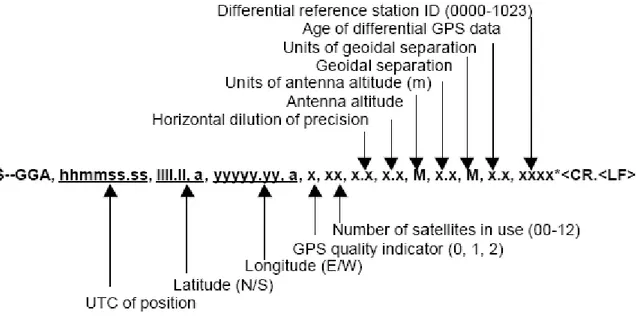
● Transmission of data between a GPS receiver and a device: The National Maritime Electronics Association (NMEA) standard for interfacing marine electronic devices covers the format for GPS output records. The standard for corrected GPS output records at the remote receiver is found under NMEA 0183, Version 2.xx. NMEA 0183 output records can be used as input to whatever system the GPS remote receiver is interfaced, (US Army, 2003). As shown in figure 2.11, the NMEA 0183 data streams may include information on position, datum, time, fix related data for a GPS receiver, and other variables.
2.2 Geographic Information System (GIS). 2.2.1 Historical review.
Geographic Information Systems arose from activities in 4 different fields, (Gottfried, 2003):
● Cartography, which attempted to automate the manually dependent map making process by substituting the drawing work by vector digitisation.
● Computer graphics, which had many applications of digital vector data apart from cartography, particularly in the design of buildings, machines and facilities.
● Data bases, which created a general mathematical structure according to which the problems of computer graphics and computer cartography could be handled.
● Remote sensing, which created immense amounts of digital image data in need of geocoded rectification and analysis. As shown in figure 2.12.
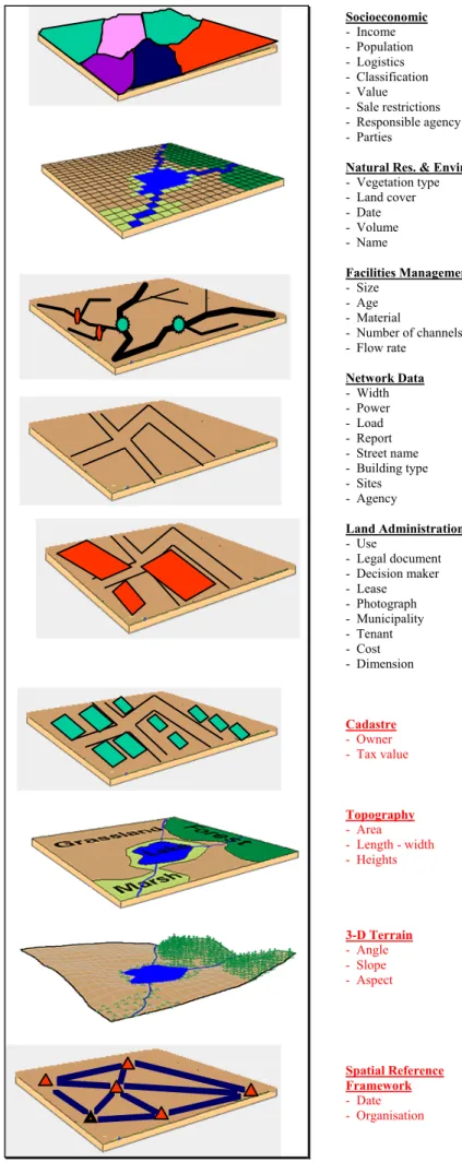
In the last century, thematic maps came into use. Thematic maps contain information about a specific subject or a theme, such as surface geology, land use, soils, political units and collection areas, as shown in figure 2.13.
Figure 2.13 Illustration of thematic layers.
The map overlay concept began to exploit thematic maps by extracting data from one map to place it onto another. As an early example, the geographic extent of the German city of Dusseldorf was mapped at different time periods in this way in 1912, and a set of four maps of Billerica, Massachusetts, were prepared as part of a traffic circulation and land-use plan in the same year. By 1922 these concepts had been refined to the extent that a series of regional maps were prepared for Doncaster, England, which showed general land use and included contours or isolines of traffic accessibility . In 1929 “survey of New York and its Environs” clearly shows that overlaying maps on top of each other was an integral part of the analysis, in this case of population and land value, (Keith, 2001).