Selçuk J. Appl. Math. Selçuk Journal of Vol. 7. No.2. pp. 27-40, 2006 Applied Mathematics
Image Enhancement In Posıtron Emıssıon Tomography Usıng Expec-tation Maxımızatıon
Halil Erol1, Etem Köklükaya1Ahmet ALKAN2
1Electric-Electronics Engineering Dept. Sakarya Üniversitesi, Adapazar, Türkiye e-mail: haerol555@yaho o.com
2Department. of Computer Engineering, Ya¸sar University, ˙Izmir, Türkiye e-mail: ahm et.alkan@ yasar.edu.tr
Summary
Positron Emission Tomography (PET) tomography is one of the imaging modal-ity. PET Tomography scanners collect measurements of a patient’s in vivo radiotracer distribution. These measurements are reconstructed into cross-sectional images. Tomographic image reconstruction forms images of functional information in nuclear medicine applications and the same principles can be applied to modalities such as X-ray computed tomography and Single Photon Computed Tomography(SPECT).
Reconstruction in PET can be done in two ways, direct and algebraic methods. Iterative reconstruction is an algebraic reconstruction method. The great advan-tage of iterative methods is that correction to attenuation and depth-dependent detector response can be incorporated to the reconstruction process. One of the drawbacks of the iterative reconstruction methods is the huge computation, due to large system matrices. This system matrix is very sparse. In Matlab 7, matrices having elements more than 100 million can not be executed or stored due to its size restriction. To overcome this problem we have implemented a new storage technique. By this technique, large system matrices can be manipulated in Matlab7.
Reconstructed images are compared with the images which are obtained by using direct reconstruction algorithms, namely, Filtered Backprojection. Key words: PET tomography, image reconstruction, iterative reconstruction methods.
The PET is an imaging technique, which is potentially useful in study of human physiology, organ functions and especially in tumor detection. PET aims at ob-taining a quantitative map of spatial and temporal distribution of radio-nuclides inside the human body by measuring the event counts of positron-electron anni-hilation. The PET images can be reconstructed by either analytic methods such as filtered backprojection algorithm or iterative algorithm such as Algebraic Re-construction Technique(ART), Expectation Maximization(EM). The main parts of analytic methods are filtering and backprojection. Iterative methods, on the other hand starts with initial guess of the solution and iteratively updates the object according to computed pseudo-projections and measured projection data. But, the time for reconstruction of images using iterative methods for obtaining acceptable image is very high. On the other hand iterative methods have the following advantages; Linear algebra is very strongly supported in mathematics; it can be used for both 2D and 3D PET reconstructions. Limited line orienta-tion (i.e., irregular scanner geometry) is very bad for the direct methods, and with (the linear algebra approach, problems with missing data in the sinogram can easily be incorporated into the matrix formalism. A finite, i.e. non-zero detector size can be modeled into the system, hence the model need not based on a ray approximation, and varying detector sensibility can in principle be modeled into the system of equations, hence, better modeling of the physical scanner setup is possible.
2. Projection And Backprojection Operator
The collimator allows only photons whose direction is parallel to the axis of its holes to be potentially detected. For each detector angle , and for each location on the detector, this direction is defined by a line 0 whose equation
is: (1) 1= 1= and 1− = (2) − 1=
then combining equation (1) and (2) to get rid of x1and y1
x = cos - u sin y= sin - u cos
∙ ¸ = ∙ − − ¸ ∙ ¸
= + (3)
= − +
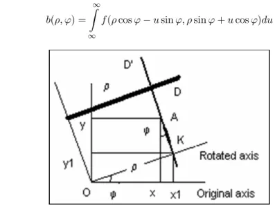
Let us first consider the projection operation, giving the number of counts de-tected in any point of the detector line (, ) as a function of the number of counts (, ) emitted in any point of the field of view. Mathematically, the projection operator can be defined by the Radon transform. The Radon trans-form (, ) of a function (, ) is the line integral of the values of (, ) along the line inclined at an angle from the -axis at a distance from the origin:
(4) ( ) =
∞
Z
∞
( cos − sin sin + cos )
Figure 1: Geometrical interpretation of photon acquisition in two dimensional PET with septa. The aim is to find in the field of view the set of points A(, ) that perpendicularly projects on . Distance AK is u. Rotated axis is degree shifted version of the original axis. D is representing the detector.
Because an integral is basically a sum of values, the value (, ) is the sum of the values (, ) along 0. For this reason, (, ) is called a ray-sum.
The variable defines the location of the points to be summed (the points along 0). Because computers can only deal with a finite number of elements in the detector and in the field of view, (, ) and (, ) are in practice functions of discrete variables–that is, the variables , , , and have a finite number of possible values. Here, the elements of the slice are the pixels, and each point of measurement on the detector, for each projection angle, is called a bin. So the number of bins equals the number of points of measurement multiplied by
the number of angles. Below there is an example of a discrete projection for a 4 x 4 image at 2 angles(0 and 90).
= ⎡ ⎢ ⎢ ⎣ 1 3 2 4 5 1 2 3 2 4 6 8 4 8 2 1 ⎤ ⎥ ⎥ ⎦ == ⎡ ⎢ ⎢ ⎣ 1 2 3 4 5 6 7 8 9 10 11 12 13 14 15 16 ⎤ ⎥ ⎥ ⎦ b11=x1+x2+x3+x4=10, b12=x5+x6+x7+x8 =11 b13=x9+x10+x11+x12=20,b14=x13+x14+x15+x16=15 b24=x4+x8+x12+x16=16, b23=x3+x7+x11+x15=12 b22=x2+x6+x10+x14=16, b21=x1+x5+x9+x13=12
Value in each bin is sum of values of pixels that project onto that bin. The result is a sinogram with 2 columns (corresponding to 2 projection angles) and 4 rows (corresponding to 4 points of measurements on the detector), so there are 8 bins. For example: b1=x1+x2+x3+x4 and b2=x5+x6+x7+x8. Result of
projection is sinogram with 2 columns, whose values are (10, 11, 20, 15 ) and (12, 16, 12, 16). In matrix form; = ∙ 10 11 20 15 12 16 12 16 ¸
But two projection angle is not enough for reconstruction, at least 16(4*4) projections needed.
A common representation for the projection data corresponding to a slice is the sinogram. A sinogram is a 2D image, in which the vertical axis represents the count location on the detector, and the horizontal axis corresponds to the angular position of the detector. The corresponding number of counts is assigned to each point of the sinogram. From a mathematical point of view, the sets of values in the sinogram and the reconstructed slice can be considered as matrices or vectors. From now on, the sinogram and the slice are considered as two vectors; the vectors are formed by stacking the rows of the matrices. In these vectors, the location of a bin is known by its index and the location of a pixel by its index . It can be shown that the vector is the matrix product of matrix and vector . The value of any bin is a weighted sum of the pixel values
in the image: (5) = 11+ 22+ 33+ + a= X =1
This is the discrete formula for the projection operation, and the essential point here is that the discrete projection operation can be defined as a matrix product. This product can be concisely written as b= Af, where is called the forward projection operator . In other words, the projection operation allows one to
find the sinogram for the given slice. The point here is that any aij can be seen as a weighting factor representing the contribution of pixel to the number of counts detected in bin , or as the probability that a photon emitted from pixel is detected in bin . The use of zeros or ones in the matrix can be interpreted as the binary choice “a given pixel contributes or does not contribute to the number of counts detected in any bin”. However, to get a more realistic model, we want to be able to modulate this contribution. To do so, the 0
s may
not be necessarily equal to 0 or 1 but can be any real values between 0 and 1. As we shall see below, the correct determination of the 0
s is important
because the iterative algorithms use the projection operation. The values are carefully chosen to take into account the geometry of acquisition and, more precisely, the fact that a variable fraction of a pixel contributes to the counts detected in a given bin, depending on their relative positions and the angle of acquisition. Below, pixel driven approach is explained in detail. Moreover, the camera response and physical phenomena such as attenuation and scatter can be efficiently modeled by choosing the appropriate values for the ’s. The
capability to account for physical phenomena and for a non-ideal imaging system is one of the advantages of iterative approaches compared with the FBP method. Without loss of generality we focus on the 2D case. A cross section can be divided into N square pixels, represented by an N-dimensional column vector f. Each pixel has a constant linear attenuation coefficient f = 1, . . . ,N.
Sim-ilarly, projection data can be assembled into an M-dimensional column vector b, with the element being = 1, . . .,M.
Let = () be the matrix mapping f to , where measures the contribution
of f to . We have the following linear system:
(6) =
We are interested in finding a vector that is a solution of = Af. Theoretically, direct methods exist to solve the system = Af. A method called direct inversion consists in the determination of the inverse of , noted −1, because =
−1. This method has several flaws: (a) It is computationally intensive for
current computers, even for 64 x 64 images; The matrix is normally very large, eg., 1002x 1002elements, thus calculation of a generalized inverse of is
extremely costly both in time and memory (b) −1 may not exist; (c) −1
may be not unique; (d) −1 may be ill-conditioned–i.e., small changes in the
data may produce large differences in the result ;for example, when is noisy. Unfortunately, in practice, the matrix is ill-conditioned, because of the noise in the projections. The system matrix will be (near) singular, i.e.. have very small singular values, i.e.. that reconstruction written in the linear algebra formalism is an ill-conditioned problem. Some of the image values can be under determined and others very over determined due to the uneven coverage of the projections (sinogram lines) in the image domain. This problem must then be
controlled with constraints and/or regularization. The system matrix will be sparse due to the fact, that only approximately of the x image pixels adds weight to a certain bin in the sinogram. Thus, the direct methods are not widely employed.
The system matrix is in general not quadratic (i6=j ), which limit the number of techniques applicable if not forming the normal equations. It turns out that does not have a simple structure, such as a band matrix, hence the inversion of have to use rather slow methods. The reason that does not have a simple structure is partly due to the easy sorting schemes, another reason is that line parameters does not have a very simple relation to the image coordinates 3.Materıal And Method
3.1The Calculation of Matrix Elements
The matrix can be estimated in several ways. The contribution of a given pixel to a given bin is variable, because it depends on their relative positions and the angle of acquisition. This has to be taken into account during the backprojection. At least 3 practical solutions exist: With the ray-driven method [1], the value in each bin (i.e., the ray-sum) is added to the image at pixels the ray goes through, but the addition is weighted according to the ray length in each pixel. One very common approach is to use a nearest neighbor approximation. Here pixel driven nearest neighbor approximation is used. But a first order pixel oriented interpolation approximation can also be used. Other alternative methods can also be found in literature. A good interpolation scheme takes longer time compared to the coarse interpolation schemes.
3.2Pixel or voxel driven nearest neighbor approximation approach:
If the image pixel is considered as a square it is 2D, if it is considered as a cube it called as voxel (3D). For simplicity 2D notation is used. Around each pixel (x,y) is placed in a square ∆x*∆x wide.
(7) 0= − cos − sin
Here is the distance of the projection rays to the origin, as shown in figure 1. ’ is the distance between the projection ray passing through the pixel and the pixel origin. |0cos | ∆ 2 | 0sin | ∆ 2 =⇒ + += 4
If the line with parameters (,) crosses the square, the matrix element a is
set to ∆x, otherwise it is set to zero 3.3EM Algorithm
The principle of the iterative algorithms is to find a solution by successive es-timates. The projections corresponding to the current estimate are compared with the measured projections. The result of the comparison is used to modify the current estimate, thereby creating a new estimate. The algorithms differ in the way the measured and estimated projections are compared and the kind of correction applied to the current estimate. The process is initiated by arbi-trarily creating a first estimate; for example, a uniform image initialized to 0 or 1 (depending on whether the correction is carried out under the form of an addition or a multiplication).
The aim is to solve = Af, where is the vector of values in the sinogram, is a system matrix, and is the unknown vector of pixel values in the image to be reconstructed. Measurements are subject to variations due to the Poisson probabilistic phenomena of the radioactive disintegrations. As a consequence, a dataset corresponds to a particular measurement; when the probabilistic phenomena are not taken into account, is the particular solution corresponding to that particular measurement . The goal of the EM algorithm is to find a “general” solution as the best estimate for : the mean number of radioactive disintegrations ¯ in the image that can produce the sinogram with the highest likelihood [2-4]. This can be done using the Poisson law that allows one to predict the probability of a realized number of detected counts, given the mean number of disintegrations. Thus, each iteration of the algorithm is divided into 2 steps: in the expectation step, the formula expressing the likelihood of any reconstructed image given the measured data is formed,
() = () = Y =1 (∗) ! −∗
and the maximization step, the image that has the greatest likelihood to give the measured data is found [4].
() = − X =1 + X =1 P 0=100 = −1 + X =1 P 0=100 = 0
This leads to the EM algorithm as described by Lange and Carson [2]
(9) ()= (−1) P 0=10 X =1 P 0=10(−1)
The first image (initialization of f) can be a uniform disk enclosed in the field of view [5] or an image obtained by FBP (in this case the negative values, if any, must be set to zero or some small positive value). Notice that because the first image is positive (negative values do not make sense) and because each new value is found by multiplying the current value by a positive factor, any ()
cannot have negative values and that any values set initially to zero will remain zero.
The EM algorithm can be seen as a set of successive projections/backprojections[6]: The weight factor
= P
−1
is the ratio of the measured number of counts to the current estimate of the mean number of counts in bin and r* is the backprojection
of this ratio for pixel .
In other words, at each iteration , a current estimate of the image is available. Using a system model (which may include attenuation and blur), it is possi-ble to simulate what projections of this current estimate should look like. The measured projections are then compared with simulated projections of the cur-rent estimate, and the ratio between these simulated and measured projections is used to modify the current estimate to produce an updated (and hopefully more accurate) estimate, which becomes iteration +1. This process is then repeated many times. The EM algorithm converges slowly and may require 20-50 iterations. Note also that the EM algorithm is nonlinear, hence addi-tive noise the sinogram will not automatically lead to an addiaddi-tive noise in the reconstructed images.
Equation (9) is very closed form, it can be decomposed in to four parts
(10) = (−1) (11) = (12) = (13) ()= (−1)
As can be seen from eqn(11) that if b has a value zero this can led to instability.
Algorithm 1.1: Construction of system matrix
when i corresponds to a line not entering region of activity, hence the forward projected value b becomes zero, thus the denominator in eqn(11) is a potential
instability problem.
4.Results And Discussion
Reconstruction in PET can be done in two ways; direct and algebraic methods. Direct reconstruction methods offer an analytic mathematical solution for the formation of an image. The most common direct reconstruction methods are fil-tered backprojection and filtering after backprojection. Iterative reconstruction is an algebraic reconstruction method. The great advantage of iterative meth-ods is that correction to attenuation and depth-dependent detector response can be incorporated to the reconstruction process. One of the drawbacks of the iterative reconstruction methods is the huge computation, due to large system matrices. System matrix A is very large matrix. For example, to reconstruct
81x81 image, the size of the system matrice is nearly 9639x6561(since it depends on number of projection angles and radial samples). This system matrix is very sparse, at most ten percent of the values are different than zero. In Matlab 7, matrices having elements more than 100 million can not be executed or stored due to its size restriction. Almost more than 80x80 pixel images can not be exe-cuted in Matlab environment. In order to get an accurate image, this resolution is low. To overcome this problem we have implemented a new storage technique. By this technique, large system matrices can be manipulated in Matlab7. In our implementation, instead of storing full matrice elements only nonzero elements are stored. The system matrix is divided into two parts. One of them is used to restore indices positions that have a nonzero value, and the other is used to restore the value accumulated at that indices.
Figure 2. 81x81 pixel Shepp-Logan phantom
Expectation Maximization (EM) method is used in reconstruction part. During reconstruction process, system matrix is reorganized into original position row by row or column by column, whatever needed. In algorithm 1 flowchart of generation of system matrix is explained. In algorithm 2, one iteration of EM algorithm is explained.
In this research we implemented EM algorithm and reconstructed the Shepp-Logan phantom images. Firstly 81x81 pixel Shepp-Shepp-Logan phantoms’
0 0.05 0.1 0.15 0.2 0.25 0.3 0.35 0.4 x y örüntü -1 -0.8 -0.6 -0.4 -0.2 0 0.2 0.4 0.6 0.8 1 -1 -0.8 -0.6 -0.4 -0.2 0 0.2 0.4 0.6 0.8 1
Figure 3. 81x81 pixel Shepp-Logan phantom is reconstructed by EM algorithm with 2 iteration. 0 0.1 0.2 0.3 0.4 0.5 0.6 0.7 x y örüntü -1 -0.8 -0.6 -0.4 -0.2 0 0.2 0.4 0.6 0.8 1 -1 -0.8 -0.6 -0.4 -0.2 0 0.2 0.4 0.6 0.8 1
Figure 4. 81x81 pixel Shepp-Logan phantom is reconstructed by EM algorithm with 3 iteration.
0 0.1 0.2 0.3 0.4 0.5 0.6 0.7 x y örüntü -1 -0.8 -0.6 -0.4 -0.2 0 0.2 0.4 0.6 0.8 1 -1 -0.8 -0.6 -0.4 -0.2 0 0.2 0.4 0.6 0.8 1
Figure 5. 81x81 pixel Shepp-Logan phantom is reconstructed by Filtered Backprojection algorithm with Hann filter is used.
image is generated then sinogram of this image is obtained. This sinogram is used in reconstruction process. To compare reconstructed images with conven-tional methods, images are also reconstructed by using Filtered Backprojection algorithm. Hann filter is used in Filtered Backprojection algorithm as a filter type. 0 0.1 0.2 0.3 0.4 0.5 x y örüntü -1 -0.8 -0.6 -0.4 -0.2 0 0.2 0.4 0.6 0.8 1 -1 -0.8 -0.6 -0.4 -0.2 0 0.2 0.4 0.6 0.8 1
Figure 3. 101x101 pixel Shepp-Logan phantom is reconstructed by EM algorithm with 1 iteration.
In EM a mask is used which is useful for circular and elliptical phantoms. The values of masked pixels are taken as zero. This has a contribution in reducing
the computation time of reconstructed images. Elapsed time is 4,5 minute for one iteration EM of 81x81 image in P4 2800Mhz PC. Reconstruction of the same image by using Filtered Backprojection method took one minute. But the image quality of EM algorithm is better than the FBP. Reconstruction of 101x101 image for one iteration in AMD athlon64 2800 took 2568 minute. Separation of the system matrix caused elongation of the execution times
.
5.Conclusıons
In this research we implemented EM algorithm and reconstructed the Shepp-Logan phantom images. We used reconstructed images of the same size to compare the algebraic reconstruction with the direct reconstruction method. Least error is achieved in algebraic reconstruction method by using EM.
References
1. Siddon RL. Fast calculation of the exact radiological path for a three-dimensional CT array. Med Phys. 1985;12:252—255.
2. Lange K, Carson R. EM reconstruction algorithms for emission and trans-mission tomography. J Comput Assist Tomogr. 1984;8:306—316.
3. Kaufman L. Implementing and accelerating the EM algorithm for positron emission tomography. IEEE Trans Med Imaging. 1987;MI-6:37—51.
4. Shepp LA, Vardi Y. Maximum likelihood reconstruction for emission tomog-raphy. IEEE Trans Med Imaging. 1982;MI-1:113—122.
5. Llacer J, Veklerov E, Coakley K, Hoffman E, Nunez J. Statistical analysis of maximum likelihood estimator images of human brain FDG PET studies. IEEE Trans Med Imaging. 1993;12:215—231
6. J. Nuyts, “On estimating the variance of postsmoothed MLEM images,” IEEE Trans. Nucl. Sci., vol. 49, pp. 714—721, June 2002.