A producer-centric caching strategy for named data networking

(1)

A PRODUCER-CENTRIC CACHING

STRATEGY FOR NAMED DATA

NETWORKING

a thesis submitted to

the graduate school of engineering and science

of bilkent university

in partial fulfillment of the requirements for

the degree of

master of science

in

computer engineering

By

H¨

useyin A¸cacak

September 2018

(2)

A Producer-Centric Caching Strategy for Named Data Networking By H¨useyin A¸cacak

September 2018

We certify that we have read this thesis and that in our opinion it is fully adequate, in scope and in quality, as a thesis for the degree of Master of Science.

˙Ibrahim K¨orpeo˘glu(Advisor)

¨

Ozg¨ur Ulusoy

Ahmet Co¸sar

Approved for the Graduate School of Engineering and Science:

Ezhan Kara¸san

(3)

ABSTRACT

A PRODUCER-CENTRIC CACHING STRATEGY FOR

NAMED DATA NETWORKING

H¨useyin A¸cacak

M.S. in Computer Engineering Advisor: ˙Ibrahim K¨orpeo˘glu

September 2018

With growing number of users and content on Internet, the existing Internet architecture needs to evolve to be more efficient to find and carry content, and Named Data Networking (NDN) is a new Internet architecture aiming to achieve this. Named Data Networking focuses on data directly instead of considering servers and their locations to retrieve data. It adopts the paradigm of requesting and retrieving data with name instead of delivering a packet to a specific des-tination address. In NDN, caching of data in intermediate network nodes can help moving data closer to the consumers and in this way can be very effective in reducing application response time and network bandwidth consumption. For this, proper cache placement and replacement strategies are needed. In this the-sis, we propose a producer-centric in-network caching strategy, called PCDC, to efficiently and effectively cache data in the intermediate nodes of a named data network. In our scheme, intermediate nodes that are at the intersections of mul-tiple consumer paths are selected as caching points to cache requested data. We propose the necessary mechanisms and algorithms to select such caching points, considering the practical constrains of NDN protocols. We simulated our scheme in ndnSIM/ns3 and did extensive simulation experiments to evaluate its perfor-mance. The simulation results show that our scheme is feasible and practical to apply and is efficient in terms of increasing packet diversity and average hit-ratio, and decreasing application response time and network bandwidth consumption.

Keywords: named data networking, cache placement, caching, cache usage, inter-net of things.

(4)

¨

OZET

ADLANDIRILMIS

¸ VER˙I A ˘

GLARI ˙IC

¸ ˙IN ¨

URET˙IC˙I

MERKEZL˙I ¨

ON BELLEK STRATEJ˙IS˙I

H¨useyin A¸cacak

Bilgisayar Mühendisli˘gi, Yüksek Lisans Tez Danı¸smanı: ˙Ibrahim Körpeo˘glu

Eyl¨ul 2018

Mevcut ˙Internet mimarisi, internette giderek artan sayıda kullanıcı ve i¸cerikle birlikte, i¸ceri˘gi bulmakta ve ta¸sımakta daha verimli olmak i¸cin geli¸smelidir. Ad-landırılmı¸s Veri A˘gı (NDN) bunu ba¸sarmayı ama¸clayan yeni bir internet mi-marisidir. Adlandırılmı¸s Veri A˘gı, verileri almak i¸cin sunucuları ve konumlarını dü¸sünmek yerine do˘grudan veri üzerinde odaklanır. Bir paketin belirli bir hedef adrese teslim edilmesi yerine isim ile veri talep etme ve alma paradigmasını ben-imser. NDN’de, ara a˘g dü˘gümlerindeki verilerin önbelle˘ge alınması, verilerin tüketicilere daha yakın bir yere ta¸sınmasına yardımcı olabilir ve bu ¸sekilde uygu-lama yanıt süresinin ve a˘g bant geni¸sli˘gi tüketiminin azaltılmasında ¸cok etkili olabilir. Bunun i¸cin uygun önbellek yerle¸stirme ve de˘gi¸stirme stratejileri gerek-lidir. Bu tezde, biz adlandırılmı¸s bir veri a˘gındaki ara dü˘gümlerdeki verileri ver-imli ve etkili bir ¸sekilde önbelle˘ge almak i¸cin PCDC adı verilen, üretici merkezli a˘g i¸ci önbelle˘ge alma stratejisi öneriyoruz. Bizim ¸semamızda, ¸coklu tüketici yol-larının kesi¸sme noktalarındaki ara dü˘gümler, istenen verileri önbelle˘ge almak i¸cin ¨

onbellekleme noktaları olarak se¸cilmi¸stir. NDN protokollerinin pratik kısıtlarını dikkate alarak, bu tür önbellekleme noktalarını se¸cmek i¸cin gerekli mekanizmaları ve algoritmaları öneriyoruz. S¸emamızı ndnSIM / ns3’te simüle ettik ve perfor-mansını de˘gerlendirmek i¸cin kapsamlı simülasyon deneyleri yaptık. Simülasyon sonu¸cları, plan ¸ce¸sitlili˘ginin ve ortalama isabet oranının artırılması, uygulama yanıt süresinin ve a˘g bant geni¸sli˘gi tüketiminin azaltılması a¸cısından uygulan-abilir ve uygulanmasının pratik oldu˘gunu göstermektedir.

Anahtar sözcükler : anlandırılmı¸s veri a˘gları, önbelle˘ge yerle¸stirme, önbelle˘ge alma, önbellek kullanımı, nesnelerin interneti.

(5)

Acknowledgement

I would like to take this opportunity to express my gratitude to my supervisor, Prof. Dr. ˙Ibrahim K¨orpeo˘glu, for his motivation, guidance, encouragement and support throughout my studies.

I would like to thank to Prof. Dr. ¨Ozg¨ur Ulusoy and Prof. Dr. Ahmet Co¸sar for kindly accepting to spend their valuable time to review and evaluate my thesis.

Most importantly, I would like to express my gratitude to my beloved mother Hafize, father Ahmet, brother Fatih and sister Beyza. I am truly thankful for their support and love.

Finally, I want to thank my wife M¨unevver with whom I share so many things. She has a huge share in whatever I have achieved in my graduate study. I am doubtlessly grateful to her.

(6)

List of Figures

2.1 Interest Packet Structure. . . 7

2.2 Data Packet Structure. . . 8

2.3 Forwarding process of a node. . . 9

2.4 CS Table Entry Structure. . . 10

2.5 FIB Table Entry Structure. . . 11

2.6 ndnSIM Structure [1]. . . 16

3.1 Data Packet Structure. . . 25

3.2 Interest Packet Structure. . . 26

3.3 Packet Path Table Content Structure. . . 29

3.4 Sample Topology with 2 Consumers and 1 Producer. . . 30

3.5 Sample Topology with 3 Consumers and 1 Producer. . . 31

4.1 Cache Usage Ratio with Node Count. . . 38

(10)

LIST OF FIGURES x

4.3 Hop Average with Node Count. . . 39

4.4 Average Hit with Node Count. . . 39

4.5 Cache Usage Ratio with Cache Size. . . 40

4.6 Packet Diversity with Cache Size. . . 40

4.7 Hop Average with Cache Size. . . 41

4.8 Hit Average with Cache Size. . . 41

4.9 Cache Usage Ratio with Consumer Count. . . 42

4.10 Packet Diversity with Consumer Count. . . 43

4.11 Hop Average with Consumer Count. . . 43

4.12 Hit Average with Consumer Count. . . 44

4.13 Hop Average with Consumer Count. . . 44

4.14 Decrease in Network Load with Consumer Count. . . 45

4.15 Hop Average with Node Count. . . 45

(11)

List of Tables

(12)

Chapter 1 Introduction

In its early days, the main aim of Internet was to exchange information via emails and to provide communication between end users working on computers. Therefore, the Internet architecture was based on client server communication. Every end user had an IP address. In todays world, the Internet architecture still uses IP addresses. However, the number of Internet users has increased exponentially and the usage purpose of the Internet has changed drastically over the decades. A lot of applications are content centric and the users of these applications do not care about where the content comes from but cares about the content itself. This need has triggered the design of a new network architecture called Named Data Networking (NDN), which is similar to but more general than Content Delivery networks (CDNs).

Meanwhile, the concept of Wireless Sensor Networks (WSN), and later the the concept of Internet of Things (IoT) [2] have emerged. IoT is a significant innovation that will change our world and lives drastically. It is a vision of connecting all the things in the world with each other, that is, it is expected to be a giant network of a lot of different types of physical objects, such as devices, home appliances, vehicles and smart grids. The list can be extended with other things like sensors, actuators and embedded devices.

(13)

IoT architecture is composed of three parts; the perception, network and the application layer [3]. First part, the perception, has physical devices such as sensors and actuators. In this layer, the data is digitized and transmitted from/to the network part. The network part provides the communication of devices. The last part, application layer, is responsible for the resource and data management, data processing, and providing services for end users.

Host-to-host communication paradigm and Internet Protocol (IP) are success-fully used for traditional networking applications. IoT devices and applications, however, are different from traditional Internet devices. Therefore, the shift from a network architecture with IP addresses to content-centric networks fits the re-quirements of an IoT network. For instance, most of the IoT devices request data from one or more data producers without specifying any IP address. As the IoT network grows, the data volume and traffic is expected to increase as well. IoT devices have limited storage capacity, power and mobility. Therefore, named data networking is a promising architecture for solving networking related problems of IoT [4].

Named Data Networking is an approach for the future internet architecture [5]. It is a new network architecture and changes the role of the network from “deliver-ing a packet to a specific destination address” to “request“deliver-ing and retriev“deliver-ing data with a name”. NDN gives the most importance to the content. It gives a name to each content and uses this name in requesting and forwarding the content [6]. Communication is triggered by the receivers, i.e., data consumers. Consumers, that would like to receive data, send interest packets which include the name of the requested data. When a data producer receives this interest packet, it sends back the respective data packet to the requester. In NDN the routing is done using the two tables below.

• Forwarding Information Base (FIB): This table matches the name prefixes with the outgoing interfaces.

• Pending Interest Table (PIT): Content names, incoming interfaces and other information about previously forwarded interests are kept in this table.

(14)

Things in IoT need to establish end-to-end connections to retrieve content. Since there will be a huge number of things, there will be a high volume of data produced, requested and transported in the network. The content requesters do not care about where content is and how the content comes. They only care about the content they want to receive. Similarly, content producers do not care about who will receive the content [7]. There may be many different types of contents and data items produced, stored, requested and carried. Because of this large data diversity and huge data volume, there are lot of challenges faced by the network and content producers, like efficient routing, link bandwidth limitation, congestion, delivery speed, limited power, and lack of large memory in intermediate network devices.

Caching the data inside the network can be a good approach to enable auto-matic placement of data closer to the consumers. This can reduce the load on producers and on the network, and can also decrease the latency experienced by consumers in reaching the data. If the network enables caching, then the routers can have a Content Store (CS) table. However, it is not possible to cache all the contents in NDN. This would create extensive redundant content inside the network. Also, the number of replacement operations would increase immensely. The default caching strategy, Leave Copy Everywhere (LCE), makes copies ev-erywhere without running any restriction. The only restriction is the cache size. If the cache is full, then the least recently used entry is removed and the new entry is inserted.

In this thesis, we propose an efficient and effective caching scheme that can be used in an NDN for IoT. In our caching strategy, which we call Producer Centered Data Caching (PCDC), we cache the data in limited number of nodes. For a consumer-producer pair, the data is cached only in one of the nodes in the path from producer to the consumer. Other consumers sharing the path and requesting the same data can find the data cached in this node. To decide in which node on the path from a producer to a consumer the data will be cached, we add a field to the interest packet that will keep the path info while interest packet is traveling from a consumer to a producer. On the way, the routers add their ids to the interest packet in order. When an interest packet finally reaches

(15)

a producer, the producer extracts the path info and stores it in its Packet Path Table (PPT). After insertion, the producer finds the longest suffix matching path from the PPT table. The id of the node at the end of this path is appended to the data packet. This is the node that will cache the data. Then, the data packet is forwarded towards the consumer. The node whose id is equal to the id that is stored in data packet caches the packet.

We did extensive simulation experiments to evaluate our proposal. Firstly, we compare PCDC with LCE in terms of cache usage ratio, packet diversity, hop average and average hit. We use node count, cache size and consumer count as parameters as factors whose effects are investigated . We observed that our PCDC algorithms performs better than LCE in terms of cache usage and packet diversity, almost the same in terms of hop average and average hit for various values of factor parameters. We compared PCDC with no caching (caching disabled) as well. We observed that, as expected, PCDC performs better than no caching in terms of hop average and network bandwidth load with not a very significant caching load on the network.

The thesis is organized as follows. In Chapter 2, we give brief background information about Named Data Networks and ns3/ndnSIM, which is the simu-lator we used, and also present the related work. In Chapter 3, we present our proposed solution (PCDC). We explain the modifications required to NDN base protocol and additional structures needed to decide about the nodes that will cache the data packets. In Chapter 4, we present our performance evaluation and the result of our simulation experiments. Finally, in Chapter 4, we give our conclusions and future work directions.

(16)

Chapter 2 Background and Related Work

In this chapter, we will first give some background information on Named Data Networking, NS3 - Network Simulator 3, and ndnSIM – an extension to ns3 to simulate named data networking. Then we will discuss the related work.

2.1 Named Data Networking

Named Data Networking (NDN) is a new network architecture for Internet. Un-like the traditional Internet in which users are interested in where the packets come from, in NDN users focus directly on data not the physical location where the data comes from.

2.1.1 Data/Content Naming

In Internet, the URLs are given in a hierarchical manner. As in URLs, data names are hierarchical in NDN, e.g., a video produced in Bilkent University may have the name /bilkent/videos/demo.mp4 [8]. This hierarchy also represents the relationship between data elements. For example, segment 4 of version 1

(17)

of Bilkent demo video might be named /bilkent/videos/demo.mp4/1/4. This hierarchical naming of content packets provide the network with easy scaling of the routing mechanism [8].

Producers should construct data names dynamically without having any prior knowledge of data. They should either use interest selectors with longest prefix matching in order to get the data or use a deterministic algorithm to create the same name with the producer. This name management system is one of the most important parts of NDN.

2.1.2 Types of Packets

There are two types of packets in NDN. First type of packets is interest packet. Second type of packet is data packet.

2.1.2.1 Interest Packet

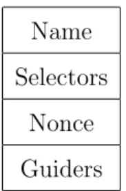
A consumer sends an interest packet with the desired data name inside it. Routers forward this interest packet towards producer(s) by looking at the data name included. The format of an interest packet is given in Figure 2.1. An interest packet has the following fields:

• Name: This field includes the desired data name. When an interest packet reaches a producer, the producer sends back the respective data packet with that contains the data with this name. The data packet follows the reverse path of the incoming interest.

• Selectors: This field is optional. There are “suffix components”, “publisher public key locator”, “exclude”, “child selector”, and “must be fresh” in this field.

(18)

The interest packet is uniquely identified with the combination of Name and Nonce. This is especially useful for avoiding looping of interest packets. • Guiders: There are “InterestLifeTime” and “ForwardingHint” as guiders.

InterestLifeTime shows the remaining time of an interest packet before it expires. The expiration time is relative to the arrival time to a intermediate node. Although it is not required, an intermediate node may subtract the time spent from the lifetime of the interest. ForwardingHint shows a dele-gation path from where the requested data can be acquired by forwarding the interest along.

Name Selectors

Nonce Guiders

Figure 2.1: Interest Packet Structure.

2.1.2.2 Data Packet

A consumer sends an interest packet whenever it needs data. When a node which has the desired data takes the interest packet, returns a data packet containing both the name of the data and the content. This data packet goes to the consumer by following the reverse path of the interest packet. The format of a data packet is given in Figure 2.2 in detail.

• Name: This field is a content name. It is formatted hierarchically and consists of sequence of name components.

• MetaInfo: This field consists of ContentType, FreshnessPeriod and Final-BlockId. ContentType, as the name suggested, shows the type of the con-tent in the data packet. First type is BLOB which is the payload identified by the name. BLOB is the default value for ContentType. Second type is

(19)

LINK which denotes a list of delegations. Third type is KEY that indicates that the content is a public key. Last type is NACK. This means that the content is an application-level NACK. The second component attached to MetaInfo field of a data packet is FreshnessPeriod. This optional compo-nent showshow long a receiving node should keep this data before making it “non-fresh”. Making it non-fresh does not mean that it is not a valid data but means that the producer might have produced newer data. If MustBeFresh field of an interest is set, then a node must not return a data that is marked as non-fresh. The last optional component of MetaInfo field is FinalBlockId that shows the final block of a sequence of fragments. • Content: The field is the content itself.

• Signature: This field binds the data name with the content together.

Name MetaInfo

Content Signature

Figure 2.2: Data Packet Structure.

2.1.3 Producer

Producer is a node that creates data packets in the network on interest request. The data packets are requested and used by consumers. The detailed information about the consumers is given below. The data packet structure is given in previous header.

2.1.4 Consumer

Consumer is a node that creates interest packets and sends to the network. These created interest packets are forwarded towards the producers. When a producer

(20)

receives an interest packet, it produces one or more data packets and sends them to the respective consumer. These data packets are used and processed in con-sumers.

2.1.5 Router Architecture

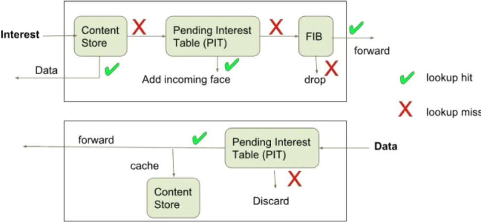
Consumers create interest packets and send them towards to producers. When an interest packet comes to a router, the router first checks its Content Store (CS) table for the corresponding data. If there is an entry for the incoming interest, the data packet is sent to the requester through the interface from which the interest packet came. Otherwise, if there is not a matching data in the CS, the router looks up the Pending Interest Table (PIT). If there is a match, the incoming interface is recorded in the entry. Otherwise, the router forwards the packet towards the producers with the help of router’s Forwarding Information Base (FIB) [9].

When a data packet arrives, the router looks up the PIT table. If there is a matching entry, the data is forwarded to all the down-stream interfaces. Then, the PIT entry is removed and the data is stored into the CS table. In this way while going to the requester, the data packet takes the reverse path of the interest. Figure 2.3 shows the forwarding process visually.

(21)

2.1.5.1 Content Store Table

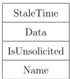
Content Store (CS) is an important feature of NDN. The success of the NDN will be depending on CS mostly [10]. The details of how CS may affect the performance of NDN will be given later as part of our proposed solution. The entry structure of a CS table is described in Figure 2.4. Each entry in CS consists of four fields that are StaleTime, Data, isUnsolicited and Name.

• StaleTime: This field denotes the stale time in milliseconds. • Data: This field contains the data itself.

• isUnsolicited: This field shows whether the data is unsolicited. • Name: This field stores the data.

StaleTime Data IsUnsolicited

Name

Figure 2.4: CS Table Entry Structure.

2.1.5.2 Forwarding Information Base Table

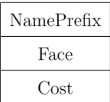
This is a table that keeps track of the faces of outgoing interest and used to send interest packets towards potential sources of requested data[11]. The details of the FIB entry structure are given in Figure 2.5. NamePrefix, Face and Cost are the fields of this table entries.

• NamePrefix: This field denotes the name prefix of the stored entry. The table is indexed by this field.

(22)

• Cost: This field is the routing cost of the corresponding outgoing face.

NamePrefix Face Cost

Figure 2.5: FIB Table Entry Structure.

2.1.5.3 Pending Interest Table

This table consists of name prefixes and their incoming faces [12]. A PIT entry may be a pending interest or a satisfied interest. The entry that keeps a pending interest is used to reach the respective data to the requester using the incoming face. The other entry that keeps the satisfied interest is used to detect loops and do some measurements [12].

2.1.6 Forwarding Strategies

NDN has built-in forwarding strategies to help various aplications and projects with different purposes to use NDN. These strategies are Best Route Strategy (BRS), Broadcast Strategy (BS) and Client Control Strategy (CCT).

2.1.6.1 Best Route Strategy

This strategy pays attention to the routing costs of the paths on the network. According to the strategy, the interests are forwarded to the upstream with lowest routing cost.

(23)

2.1.6.2 Broadcast Strategy

In this strategy, the packets are forwarded to all upstreams. If there is not a suitable upstream, the interest is rejected.

2.1.6.3 Client Control Strategy

This strategy is a consumer-driven strategy. It enables the consumers to choose outgoing interfaces of each interest.

2.1.7 Cache Replacement Policies

NDN offers many advantages for the network owners. One of them is caching in the network. Caching is to store contents on nodes closer to the requesters temporarily. The stored contents are usually the ones that are frequently accessed. Unlike traditional Internet, in NDN the contents may be cached in every node on the routes of packets. Caching provides several benefits to NDN. Firstly, the interest packets do not always go to the producer but sometimes returns from the node that has the desired data in its cache instead. The number of packets, in the network is minimized as a result. Therefore, by storing closer to the requester, overall network traffic and bandwidth usage may be decreased. Secondly, since the requested data packets are stored in the closest nodes, the response time in the network becomes very small. The last benefit is that the load on the producer may be decreased because not all packets reach to the producer.

In an NDN, caching is very important and crucial for the performance of the network. Different cache replacement policies can be used: Least Recently Used (LRU), Least Frequently Used (LFU), First In First Out (FIFO), or Random [13]. The network can also be configured as no cache.

(24)

2.1.7.1 Least Recently Used

In this policy, the entry that is not being used for the longest time is removed and the new entry is inserted into the CS table [14].

2.1.7.2 Least Frequently Used

This policy removes the entry with the lowest usage count, then inserts the new entry to the table[14].

2.1.7.3 First in First Out

As the name suggests, the oldest entry is discarded from the table and the newly arriving entry is inserted.

2.1.7.4 Random

In this strategy, the entry that will be removed from the CS is chosen randomly. The randomly chosen entry is removed and the new entry is inserted to the table.

2.1.7.5 No Cache

In NDN, although caching increases the performance of network, it is not a mandatory requirement of the network. It is possible to disable caching in an NDN.

(25)

2.1.8 Caching Strategy

This Leave Copy Everywhere (LCE) [15] strategy is the default strategy of an NDN. With this strategy, the data is cached in every node of the network that the packet passes through.

2.2 Network Simulator 3 (ns3)

As networks grow larger and become more complex, the need to simulate them with high accuracy and scalability becomes more critical [?]. Although there are large-scale network testbeds created for research, simulation programs play still very significant role, because they are more scalable, rapidly installable and repro-ducible than the real network testbeds. With simulations, the results are easily analyzable in varying conditions and parameters. The ns3 simulator (network simulator 3) is a a widely used simulator to simulate various kinds of networks. We also used ns3 in to simulate and evaluate our approach.

2.2.1 Modeling with ns3

The main goal in ns3 was to obtain realistic modes. The developers made it closer to the actual software in terms of implementations. It is developed using C++ and it facilitates the usage of C language in simulations. It also makes debugging very practical. The basic models that are used in ns3 are described below.

• Node: This model represents routers, switches, hubs, computers, or laptops.

• Device: The physical devices like Ethernet and Wireless IEEE 802.11 are modeled as device. A device connects a node to a communication channel. • Communication Channel: It is a medium that connects network devices to each other. A channel might be a point to point link or a wireless

(26)

(broadcast).

• Protocols: These are the standardized internet protocols. Before sending a packet or after receiving a packet, the packet visits protocol layers.

• Packets: These are the main units of communication in networks. The packets contain protocol information and content.

2.2.2 Result Analysis

ns3 is designed to allow users to extract customizable logs and statistics easily. It is called tracing subsystem. Users may edit this subsystem to get the desired out-puts and logs without changing anything in the core of the program. A metadata is defined to gather the run information. The information, the outputs and the configurations can be dumped in various formats. Dumped logs are used in order to draw plots and charts. Also, they can be used by external scripts and tools to analyse from different perspectives. The program is capable of drawing graphical user interfaces too. If desired, the program may run simulation visually.

2.3 ndnSIM

The ndnSIM simulator (ndnSIM) is an open source simulation development en-vironment to simulate named data networks. It is an extension to ns3. It has the following features:

• It is an open source project in order to support and assist other researchers to run NDN experiments.

• It supports almost all facilities and features of NDN.

(27)

• It is able to support considerably large simulation experiments without having any difficulty.

• It allows users to make network-layer experimentations. Routing, caching, forwarding and congestion can easily be simulated.

ndnSIM conforms to the NDN architecture. It is developed as a network layer protocol [16]. Therefore, it can run on different link-layer protocols, such as CSMA, point-to-point, and wireless. ndnSIM is developed by using object oriented programming and has modular structure. Having modular behavior provides users to be able to change desired parts without affecting other parts. General structure of ndnSIM is shown in Figure 2.6.

Figure 2.6: ndnSIM Structure [1].

The definitions of the elements in Figure 2.6 are given below.

• Named Data Networking Forwarding Daemon contains the followings [13]. – Forwarder is the main class and has PIT, CS and FIB tables, and

(28)

– Face is an abstraction that includes the communication rules to send or receive network packets.

– LinkService enables the translation between link layer packets and network layer packets.

– Transport provides the link service of a face with packet delivery ser-vice.

– CS is a cache table (content table) that keeps the data packets. For more information see Section 2.1.5.1

– PIT keeps track of the interest packets. For more information see Section 2.1.5.3

– FIB is used to forward interests toward the sources. For more infor-mation see Section 2.1.5.2

• AppLinkService: It is an implementation of LinkService for ndnSIM appli-cation and enables the communiappli-cation with appliappli-cations.

• NetDeviceLinkService: it is an abstraction to provide communication with other nodes.

• L3Protocol: its main goal is to initialize NFD instance for each node that is in the scenario. Also, it provides tracing utilities.

• Content Store is used to cache data contents.

• ndnSIM specific applications are the built-in NDN consumer and producer apps. They generate and sink network traffic. These applications are con-figurable with the help of parameters.

• Trace helpers are useful for gathering information about the simulation and logging it to an external source such as a text file.

(29)

2.4 Related Work

Caching is very important for the performance of NDN. Caching provides many advantages such as minimization of network traffic and bandwidth, reasonably small response time and reduction of producer load. Therefore, network caching became an important research field in Named Data Networking (NDN). Many researchers have proposed different solutions to default caching strategy LCE that caches all the contents in all en-route routers.

The authors of [17] propose a caching strategy called MPC that uses con-tent popularity and node level to improve concon-tent diversity and cache utilization. Firstly, they evaluate the caching property of nodes on the path by using some parameters and partition nodes into levels according to their caching property. Then, they assign contents to the matched nodes. In this strategy, three pa-rameters are used: betweenness centrality, hop count to the requester, and cache replacement rate. A node which has high caching property is a first level node and a node which has low caching property is a second level node. Interest packet field is modified by adding two fields. First one is node info that keeps betweenness centrality value, hop count and replacement rate. The second field is content info, that is, current request popularity ranking. These two fields are added in every node that is in the en-route of interest packet. When the interest packet reaches the producer, the producer evaluates the caching properties of the nodes along the path. Then a probability is calculated and appended to the data packet. Upon receiving the data packet, a node makes a caching decision using this probability. In this process, the strategy does not consider the effect of dynamic changes in content requests.

The work [18] proposes a probabilistic distributed caching strategy called pCasting that uses freshness of data, energy level and storage capacity of nodes. The work mainly focuses on wireless multi-hop information centric Internet of things (IoT) systems. The authors state that fresher data packets should have been prioritized in caching decision [18]. The freshness parameter is calculated as follows:

(30)

F R = 1 − currentT ime − ts f

In the formula, ts denotes the timestamp and f denotes freshness value. If

the ts equals to currentT ime then F R = 1 means that data may be considered

as freshly generated. The second parameter is cache occupancy level (OC) that can be between 0 and 1 inclusively. 1 means cache is full and 0 means cache is empty. The third and the last parameter is battery energy level (EN). This parameter also can be between 1 and 0, which means that battery is fully charged or discharged, respectively. When a node receives a data packet, it calculates the caching probability by using the given parameters. The calculation is done according to the following formula:

Fu = w1∗ ENn+ w2∗ (1 − OC)n+ w3∗ F Rn

As a result of these calculations, a probability is found. According to the calculated probability, the nodes that are on the path decide whether to cache or not. In the calculations, freshness period, energy level and occupancy level are used as parameters. However, the location of a node is an another important parameter for the caching. The authors do not take the location of nodes into account.

[19] proposes an in-network caching strategy. The strategy called CPRL is based on content popularity and router level.The authors compare their method with LCE. The method caches the content with high popularity in the node that is close to the user. This helps the method to improve the cache hit rate and reduce the average request time.

This methods uses a progressive approach. Request counts of popular contents continues to increase in time and the popular content gradually move to the nodes nearest to the user. The method uses all the default tables available in NDN: CS, FIB and PIT. In addition, the method adds a table called User Request Table (URT) to a first level router. The structure of interest packet is also modified.

(31)

Two fields are added: Content Popularity Table P Lx, and the number of routers’

hops hopsxen-route of the packet. There is a small modification done to the data

packet structure as well. A cache flag CI is added to store the cache location of the packet. In CPRL, the nodes closest to the user are called first level routers. A first level router counts the number of requests for requested content, and store content name and the count in URT.

When a user requests a content, the routers on the en-route are assigned a level. The closer they are to the user, the higher the level number they get. Initially, the popularity level and hops are set to 0 by the interest sender. After receiving the interest packet, the first router calculates the popularity level by using the following formula:

P Lx =        M - dnx/N e − 1 nx<N ∗ M 1 nx> = N ∗ M       

Then, the first router adds the calculated content popularity to the packet and makes the hops count 1. The other routers forward the interest packet by adding to route hops count. When the interest packet reaches the producer, it calculates the CI by using the following formula:

CI = round((P Lx− 1) ∗ (hopsx/M ) + 1)

After writing the CI value to the data packet, the node sends the packet back to the consumer. The routers that receive the data packet checks the CI. If CI equals to 0, a router caches the data, otherwise the router decreases the CI by 1. CPRL method caches contents in only one router along the path from user to producer. For some network topologies, this might not be very helpful to decrease response time, since data is cached in only one node.

The work [20] focuses mainly on user interest preferences. The authors analyze user behaviors to extract user interest preferences for different categories. In

(32)

their work, they consider three parameters for caching: user interest preferences, content popularity and cache size of nodes. Router routers are considered in two types: edge routers and normal routers. Edge routers are connected with multiple consumer nodes in the area. The mission of edge routers is to collect and forward content requests initiated by consumer nodes.

They use two content classification methods. One method considers the inter-nal theme of the content. More explicitly, the first method considers the type of information such as science, technology or other things. The other classification method cares about the external theme of the content, such as text, pictures or some other forms.

The main goal of the strategy is to cache contents with high popularity and high interest matching degree. Users are from different regions and their prefer-ences are not the same. The strategy takes this situation into account. By using interest matching degree and the content popularity, the routers decide whether to cache the content or not. The strategy is evaluated using only one topology. Its performance in different topologies are not given.

The authors in [21] propose a caching strategy for a ISP network (intra-ISP) with multiple gateways and multi-path routing. Their focus is to reduce inter-ISP traffic by using popularity and coordinated caching in an ISP. The name of their strategy is the Effective Multi-path Caching scheme (EMC). The authors state that the incoming user requests are generally stable during a time period and are not priori-known [21]. Therefore their caching scheme is triggered at every preset interval in order to determine the cache locations. The EMC consists of there parts: initialization, request spread and aggregation, and process of cache distribution.

In initialization part, the intra-isp caching topology is extracted from the net-work. The other parameters that are gateway, totalspace, low threshold, etc. are initialized as well. In the second part, the content requests in the network are monitored by access routers, ,and these routers record the request rates of all objects. In the last part, all routers make caching decisions. Since the algorithm

(33)

needs run at every time interval, it is not very suitable for the real-time systems.

The literature[22] proposes a caching strategy that minimizes the response time and reduces the number of cache replacements in the NDN network. In this strategy, an interest packet is sent from consumer to the routers in the network with the content name. Each receiving router checks, its content store in order to find a matching entry. If there is not matching, the packet is forwarded in the direction of producer. When the producer received the packet, it sends the packet to the gateway. At the gateway, a caching decision mechanism runs. One flag bit in the data packet is used to determine caching place. Flag is initially zero. The gateway router that takes the packet checks the flag bit. If the bit is zero, it does not cache the data packet, makes the bit value one and forwards. Therefore, the next alternate intermediate node along the path caches the packet. The strategy decreases the memory usage in the network however, the response time in the proposed strategy is greatly larger than LCE.

[6] proposes two ways to FIB problem in route caching. First way is to group the longest matched prefixes found in FIB LMP together with their superprefixes in order to forward correct interfaces. This group is called an atomic unit. The cache and replacement decisions are made on the atomic unit. The second way is to cache prefixes that are non-overlapped. This way helps to avoid cache hiding problems.

[23] proposes a Hierarchical Cluster-based Caching (HCC) strategy in order to minimize redundant cache copies and increase cache hit rate. HCC has two layers called Core Layer and Edge Layer. The routers in Core Layer are not used for caching, they are only responsible for forwarding and routing. On the other hand, the Edge Layer routers are used to cache contents. Also, the routers in the Edge Layer are categorized as more important and less important according to their betweenness centrality and content popularity. There is a clusterhead in each cluster which is in charge of caching mechanism. The clusterhead makes decisions about which content is to be cached and where according to the importance of nodes. The importance of the nodes are calculated at the beginning. Therefore, the HCC methods is not very adaptable for dynamic topologies.

(34)

In [24], the authors compares some well-known caching strategies in terms of response time, the publisher’s load and the distance to a content. The strategies are Leave Copy Everywhere (LCE) [25], which is the default strategy in NDN, Leave Copy Down (LCD) [25] that leaves a copy to the gateway close to the producer, edge-caching strategy [26] that leaves a copy to the gateway way close to the consumer, consumer-cache strategy [27] which leaves a copy to the gate-ways that are directly connected to the consumers, betweenness-centrality strat-egy [28] (as the name suggests the caching parameter is betweenness-centrality), and probCache [29] that takes the distance between consumer and producer as a parameter.

[30] proposes a caching strategy using a Bloom filter[31]. In this strategy, routers share their information of cache summaries with neighbors using a Bloom filter. When an interest comes to a router, the router sends the interest packet to the neighbor which has the requested content most probably. Although this has the advantage of avoiding duplicate contents to be stored in the neighboring routers so that the cache diversity increases, broadcasting cache summaries among neighbors creates overhead in the network traffic.

(35)

Chapter 3 Proposed Solution

As we described in Chapter 2, content caching in NDN has been studied in many works. Since the default caching strategy LCE is not very efficient, new caching strategies are proposed to optimize caching in NDN. These studies focus on dif-ferent aspects of caching and therefore try to solve difdif-ferent problems. Hence, other proposed strategies optimize NDN caching in different directions.

In this chapter, we present our proposed solution called PCDC (Producer Centric Data Caching) for efficient caching in NDN in order to optimize overall cache usage and increase packet diversity. Firstly, we outline the modifications that we made in NDN packets. Secondly, we describe the changes that we made in multicast strategy for forwarding. Then, we give information about necessary router structures and cache replacement strategy that we use in PCDC. Finally, we give detailed pseudo-code of our caching algorithm that runs in producers.

3.1 Data Packet

The purpose of the first four fields are the same with the default version of data packet format. Detailed information about these default fields were described in Chapter 2. In addition to those fields, we propose addition of a new field called

(36)

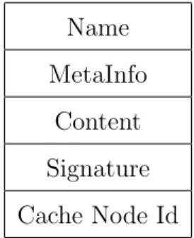
“Cache Node Id”. It denotes the id of the node where the data included in the packet should be cached. The format of the new data packet structure is shown in Figure 3.1. The new field is filled by the producer of the data packet according to the common nodes of the paths arriving interest packets have followed. After writing this common node id to the field, the producer sends the data packet into the network. When the intermediate node that has the written node id takes the data packet, it caches the data in its CS table.

Name MetaInfo

Content Signature Cache Node Id

Figure 3.1: Data Packet Structure.

3.2 Interest packet

Most of the fields of the new version of interest packet is the same as the default version. Detailed explanation of the default interest packet structure fields was given in Chapter 2. The difference is the newly added field called “Path”. In this field, we keep the ids of the nodes that are on the en-route of the interest packet. In Figure 3.2, the new interest packet structure is shown. An interest packet is created in a consumer node. Before sending the packet into the network, the consumer attaches its node id to the path field. Then the packet is sent to the network. When an intermediate node in the network receives the interest packet, the node appends its node id to path field as well. Finally, when a producer that has the corresponding data receives the interest packet, the producer extracts the path information from interest packet from the path field. In this field, the nodes on the en-route of the interest packet are in order from consumer to producer.

(37)

Name Selectors

Nonce Guiders

Path

Figure 3.2: Interest Packet Structure.

3.3 Forwarding Strategies

We use multicast strategy as the forwarding strategy. In the default multicast strategy of NDN, the intermediate nodes between producers and consumers do not change anything in arriving packets that they do not care about. In default NDN protocol, If the incoming packet is a data packet, a node checks the CS table and runs the caching algorithm. If the incoming packet is an interest packet, they insert the packet to the PIT. There is no restriction about which node caches the packet.

We have slightly modified this default strategy. In our method, there is a restriction about which node caches the packet. The data is cached only in the node that is indicated with the “cache node id” field of the data packet, otherwise the data is not cached. Since there can be multiple producers and consumers producing and consuming the same data item, the caching of a data item is not limited to only one node in the network. There may be more than one node that may cache the same data. Detailed explanation of our caching algorithm is given in Section 3.8.

A node that takes an interest packet adds its node id to the interest packet and forwards the packet to others. The algorithm for an intermediate node is given below.

The function OnIncomingInterestPacket is triggered when an interest packet reaches an intermediate node. In this function, the packet is inserted into the

(38)

PIT and the node looks its CS to determine whether there is a cache hit. If there is a hit, the respective data packet is sent to the requester. Otherwise, if there is not a hit, the interest packet is forwarded according to the FIB table.

Algorithm 1 Algorithm Triggered by On Incoming Interest Event

1: _{procedure OnIncomingInterestPacket(Packet)} 2: if LookCS(Packet) == HIT then

3: DataPacket = TakeDataPacketFromCS(Packet)

4: SendDataPacketTowardsConsumer(DataPacket)

5: else

6: if InsertPacketToPIT( Packet) == MISS then

7: if LookupFIB( Packet) == HIT then

8: AddNodeIdToThePacket(&Packet) 9: SendInterestPacket(Packet) 10: end if 11: end if 12: end if 13: end procedure

The function OnIncomingDataPacket is triggered when a data packet reaches an intermediate node. The data packet is inserted into the CS table if node id in the packet matches the id of the receiving node. Then, for every entry in PIT, the data packet is forwarded from every respective outgoing interface.

Algorithm 2 Algorithm Triggered by On Incoming Data Event

1: _{procedure OnIncomingDataPacket(Packet)} 2: if find match in PIT then

3: if cache node id in packet == own node id then 4: InsertPacketToCSTable( Packet) 5: end if 6: for EachPendingEntryInPIT do 7: SendDataPacketOutgoing(Packet) 8: end for 9: else

10: drop the packet

11: end if

(39)

3.4 Routing Structures

In an NDN, every router has a CS table, FIB table and PIT. In our work, we use all these three tables. Firstly, the CS table keeps (i.e., caches) the data that is produced by producers on the network. FIB table is used to forward an interest. It keeps track of the outgoing interfaces and their costs. Since we use multicast strategy, an interest is sent to all outgoing interfaces that are in FIB. A consumer sends out an interest packet which specifies the desired data, because NDN is requester-driven. If an intermediate router receives an interest packet, it stores the data name and the incoming interface. When the router receives the corresponding data packet, it sends out the data packet from the one or more interfaces which are recorded in PIT.

3.5 Cache Replacement Strategy

We focus on an IoT network. In an IoT network, IoT nodes are small devices and have limited capacity in terms of storage, memory, processing, and energy. The data is produced frequently by sensors and the cache capacities of nodes are not large enough to cache all data that is forwarded. We use the Least Recently Used (LRU) cache replacement strategy in our work. When a new data packet is received by a matching node in the network, if the cache of the node has enough space, the new arriving data is inserted directly to the cache. Otherwise, if the cache of the node is full, the node deletes the least recently used data entry from the cache and insert the new data item.

3.6 Producer

When an interest reaches a producer, the producer first scans the PIT table from beginning to the end in order to determine whether there is an entry that has expired stale time. If the stale time of an entry expired, it is deleted from the

(40)

table immediately. Then, producer takes the path info of the incoming interest packet and inserts it to the Packet Path Table (PPT). After the entry has been inserted, the data is prepared to be sent. The producer does not send the data packet to the network immediately, as in default version of NDN. It first finds the most common node of entries in PPT. The found node is going to be the cache node of the data packet. The cache node information is embedded into the CacheNodeId [[use consistent field naming]]] field of the data packet. This is the process of receiving interest and sending corresponding data packet in a producer. The PPT structure is given in Figure 3.3.

Path StaleTime

Figure 3.3: Packet Path Table Content Structure.

• Path: This field keeps the incoming interest packet path. For example, if the incoming interest passes through the nodes with ids 3, 2, 1 and 4, then the stored path information will be [(3),(2),(1),(4)] where 3 is consumer and 4 is producer.

• StaleTime: This field is the time when the entry will be deleted. When an interest packet arrives to a producer, the stale time in the packet and the current time are added together to find this value that will be stored in PPT table.

3.7 Consumer

We do not make any modifications on consumer side. We use the default consumer behaviour of NDN.

(41)

3.8 Proposed Caching Strategy

Our general approach is to cache the packets in the common nodes of the paths between producers and consumers. In this way, we hope more consumers can benefit from caching. In this way, unlike LCE, it is not necessary to cache data in all nodes on the paths.

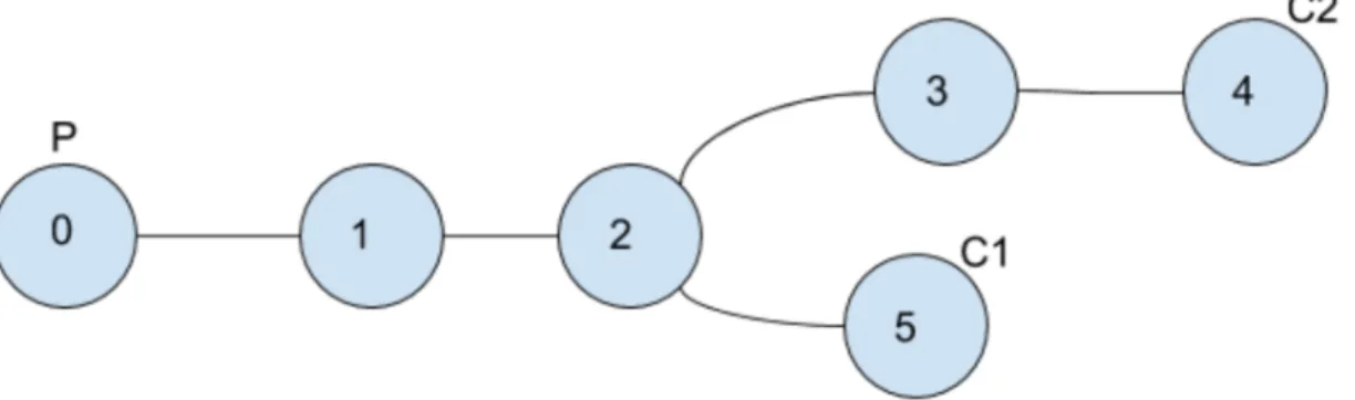
We might examine the following sample topology to give better understanding. In Figure 3.4, node 0 is a producer, node 5 is the first consumer and node 4 is the second consumer. Both two consumers requests the same data packets from the producer. First of all, they create interest packets and broadcast to the network. The interest packet of first consumer has the path of [(5),(2),(1),(0)] and the second consumer has the path of [(4),(3),(2),(1),(0)]. Let’s assume that the interest that is sent by consumer 1 arrives first. At the beginning, since there is no entry in PPT of producer, the respective data packet of the first arriving interest packet is not cached anywhere. After that, the interest packet of second consumer arrives the producer. When the producer takes this interest packet, it finds the common node of the incoming interest packet paths. In this case, the common node is node 2. Then, it inserts this node id 2 to data packets and send towards the consumers. The node 2 becomes the cache node of these two consumers. After this time, any packets that are sent by this producer to either consumer 1 or 2 are cached in node 2. In this way, if one of the two consumers requests a new data packet, it is cached in node 2 and the other consumer’s interest is replied from node 2.

(42)

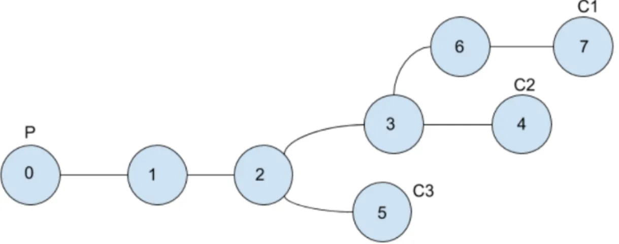
In Figure 3.5, there are one producer and three consumers. All the three consumers request the same data packet from the producer. The interest packet that is sent by consumer 1 follows the path [(7),(6),(3),(2),(1),(0)]. The interest that is sent by consumer 2 follows the path [(4),(3),(2),(1),(0)]. Finally, the interest that is sent by the consumer 3 follows the path [(5),(2),(1),(0)].

We might give an example scenario to trace the algorithm. Firstly, the con-sumer 3 sends the interest packet. At the beginning, since there is no entry in PPT of producer, the respective data packet of the first arriving interest packet is not cached anywhere. After that, the interest packet of second consumer arrives the producer. When the producer takes this interest packet, it finds the common node of the first two incoming interest packets’ paths by using the longest suffix matching. Their common node is node 2 and the respective data packet is cached in node 2. If the interest packet of consumer 1 reaches the node 2 after the data packet is cached in node 2, the response to the interest is returned from node 2, not the producer. Otherwise, if the interest packet of node 3 crosses over node 2 before caching, it reaches to the producer. The producer compares the path of the incoming interest packet with the two stored entries in PPT. It finds the longest matching and decides to cache in node 3. This cache node id is stored in the data packet and the packet is sent towards to the consumer 1. Node 3 caches the packet.

Figure 3.5: Sample Topology with 3 Consumers and 1 Producer.

(43)

the data packets.

Algorithm 3 Delete Entry with Expired Stale Time from PPT

1: _{procedure DeleteEntryFromPPT} 2: CurrentTime = GetCurrentTime()

3: // PPT is the global variable to reference the table itself

4: for i in range( 0 , PPT.size() ) do

5: // if the entry has an expired stale time, then delete it from the PPT

6: if PPT[i].GetStaleTime() <CurrentTime then

7: PPT[i] = NULL

8: end if

9: end for

10: end procedure

First, before processing an incoming interest packet or periodically, Algo-rithm 3 is run to delete obsolete entries from PPT, so that these old paths do not effect the decision process. Then, the Algorithm 4 is run to find the node to cache the data packet that will be sent as a reply to an interest. The algorithm extracts the path information from the incoming interest packet. This is the path from the consumer sending the interest to this producer. Then, the algorithm scans all the entries in the PPT (all paths) in order to find the longest matching parts of the paths. After that, the incoming interest packet path is also added to the PPT by using the Algorithm 5. Then, the packet is sent back towards the consumer.

3.9 Summary

In this chapter, we have presented our caching method that we propose for NDNs that will be used especially for IoT. We discussed our modifications to the NDN packets, multicast strategy and producer processing. We also gave the pseudo-code of our caching algorithm running in producers, that decides on where data will be cached. Our strategy is not topology dependent. Our algorithm works in any type of topology. However, the effectiveness and efficiency of our algo-rithm might change from one topology type to another. We used multi-hop mesh topologies in our experiments. In addition, our caching decision algorithm can

(44)

Algorithm 4 Finding a Cache Node Id

1: _{procedure FindCacheNodeId( InterestPacket, PPT )} 2: // initialize variables

3: Path = GetPathFromInterestPacket( InterestPacket )

4: CacheNodeId = -1;

5: CacheIndex = -1;

6: // scan all entries in PPT to find longest matching node.

7: for Each Entry in PPT do

8: TmpCacheIndex = 0;

9: if Path != Entry then

10: while TmpCacheIndex <Entry.length() and

11: TmpCacheIndex <Path.length() and

12: Path[ Path.length() - TmpCacheIndex ] == Entry[ En-try.length() - TmpCacheIndex ]

13: do

14: TmpCacheIndex = TmpCacheIndex + 1;

15: end while

16: if TmpCacheIndex - 1 >CacheIndex then

17: CacheNodeId = Path[ Path.length() - TmpCacheIndex ];

18: CacheIndex = TmpCacheIndex - 1; 19: end if 20: end if 21: end for 22: return CacheNodeId 23: end procedure

run quite frequently based on arrival of interests without creating any extra traffic and time overhead. Therefore, our method may also be used in dynamic topolo-gies. Our approach incurs considerably small overhead on data packets, interest packets and producer processing.

(45)

Algorithm 5 Inserting New Entry To PPT

1: _{procedure InsertNewEntryToPPT(InterestPacket, StalePeriod)} 2: Path = GetPathFromInterestPacket( InterestPacket)

3: CurrentTime = GetCurrentTime()

4: StaleTime = CurrentTime + StalePeriod

5: // PPT is the global variable to reference the table itself

6: // if the table has not an empty space, then run LRU algorithm to delete an entry.

7: if PPT has not an empty slot then

8: DeleteLRU()

9: end if

10:

11: for i in range( 0 , PPT.size() ) do

12: // if the index i is null, then insert the new entry and break

13: if PPT[i] == NULL then

14: PPT.insert(Path, StaleTime)

15: break

16: end if

17: end for

(46)

Chapter 4 Performance Evaluation

In order to verify the performance of our proposed caching strategy, we imple-ment the experiimple-ments and create scenarios on ndnSIM simulation platform. We have modified the packet structures and wrote the code for our caching strategy. The comparison between our proposed caching strategy and the default caching strategy LCE is made in three aspects: overall cache usage ratio, packet diversity, hop average and average hit.

4.1 Simulation Settings

We use ns3 for the simulations and experiment configurations are shown in Table 4.1.

4.2 Evaluation Metrics

We use the following evaluation metrics to compare our caching strategy with LCE.

(47)

Parameter Values # of Interests 2 / Per Second

Data Rate 1Mbps Propagation Delay 10ms PPT Size 10 PPT Stale Time 1s # of Contents 80 Simulation Time 80s # of Producer 4 # of Consumer 6, 8, 10, 12, 14 Cache Size 5, 10, 15, 20 Node Count 50, 100, 150, 200, 250 Table 4.1: Simulation Parameters and Values.

First one is average hit. It is the percentage of cache hits overall network. Total number of hits is divided by the sum of total misses and hits. Then, the result is multiplied by 100 to find percentage.

Second one is cache usage ratio. It is the percentage of overall network cache usage. After the program stops, the overall cache usage is calculated by dividing the used cache capacity to overall cache capacity. Then, the result is multiplied by 100 to find percentage.

Third metric is packet diversity. When the program stops, the number of different packets in caches overall the network are counted and divided by the number of different packets during the simulation. Then, the result is multiplied by 100 to find percentage.

Fourth metric that we use is hop average. This is the average number of hops between data providers (a node cache or a producer) and the consumers.

(48)

4.3 Simulation Results and Performance

Evalu-ation

Experiments on different metrics are carried out in order to illustrate the perfor-mance of our caching strategy.

4.3.1 Node Count

Below graphs examine the effect of node count on PCDC and LCE strategies. In this test, we use 4 producers and 6 consumers. Each producer creates different data. 2 consumers request the data packet from the first producer. The other 2 consumers request the data packet from the second producer. The fifth consumer requests the data from the third producer. The sixth consumer requests the data from the fourth producer. Cache size is 10 and the simulation runs for 50 nodes, 100 nodes, 150 nodes, 200 nodes and 250 nodes.

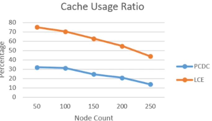
Figure 4.1 shows the comparison of two strategies in terms of cache usage ratio. As can be seen from the figure, PCDC strategy uses approximately 30% of the cache capacity of overall network and LCE uses 75% of the cache capacity of overall network when there are 50 nodes. As node count increases, the overall cache capacity of the network increases and the number of nodes that the data packets pass does not increase as much as the node count grows. Therefore, the cache usage ratios decrease for both algorithms as the node count increases. PCDC strategy has cache usage ratio less than LCE for all node counts.

The comparison of the two strategies in terms of packet diversity is shown in Figure 4.2. In a network, the more number of nodes, the more cache capacity. The number different packets cached in the nodes substantially depends on the cache capacity of the network. It can be seen from the figure that the packet diversity goes up with the rising of node count and the packet diversity of PCDC strategy is greatly larger than LCE for all node counts.

(49)

Figure 4.1: Cache Usage Ratio with Node Count.

Figure 4.2: Packet Diversity with Node Count.

In Figure 4.3, the two strategies are compared in terms of hop average. The number of total hops which data packets come is directly related to where data packets are cached. Cache strategies try to cache data packets closer to consumers as possible. Since the cache capacity is limited, it is not possible to cache all data packets next to consumers. PCDC is successful for caching contents closer to consumers according to the test results. As can be seen from the figure, the hop average in PCDC is always less than LCE for all node counts.

In Figure 4.4, the two strategies are compared in terms of average hit. In a network, network owners want to increase cache hit so that the data requesters get data as soon as possible. In our case, average hit in PCDC is lager than LCE for all node counts.

(50)

Figure 4.3: Hop Average with Node Count.

Figure 4.4: Average Hit with Node Count.

4.3.2 Cache Size

Below graphs examine the effect of cache size on PCDC and LCE strategies. In this test, we use 4 producers and 6 consumers. Each producer creates different data. 2 consumers request the data packet from the first producer. The other 2 consumers request the data packet from the second producer. The fifth consumer requests the data from the third producer. The sixth consumer requests the data from the fourth producer. The simulation runs for cache sizes of 5, 10, 15, and 20.

Figure 4.5 shows the comparison of two strategies in terms of cache usage ratio. As can be seen from the figure, PCDC strategy uses approximately 25% of the cache capacity of overall network and LCE strategy uses almost 60% of the cache

(51)

capacity of overall network for all cache sizes. As cache size increases, the overall cache capacity of the network increases proportionally. However, the cache usage ratio stabilized for all cases because the cache nodes continue to full their caches and do not change much.

Figure 4.5: Cache Usage Ratio with Cache Size.

The comparison of the two strategies in terms of packet diversity is shown in Figure 4.6. Packet diversity of PCDC strategy is considerably larger than LCE strategy. It is 70% and 30% for the cache size 5 in PCDC and LCE strategies, respectively. As the cache size increases, the packet diversity of two strategies in-crease because caches keep more packets in their storage. PCDC strategy almost stabilizes after the cache size of 15 at 100% and LCE reaches 90% for the cache size of 20.

Figure 4.6: Packet Diversity with Cache Size.

(52)

average in PCDC strategy is much smaller than the hop average in LCE. Since cache size increases and there are more caching places, the hop count average in overall network decreases in both strategies.

Figure 4.7: Hop Average with Cache Size.

In Figure 4.8, the two strategies are compared in terms of Hit Average. Hit average in PCDC strategy is greater than the hit average in LCE. In addition, the average hits for the two algorithms increase because the packet diversity increases all over the network and the network is more capable of keeping different packets in caches.

(53)

4.3.3 Consumer Count

Below graphs examine the effect of cache size on PCDC and LCE strategies. In this test, we use equal the cache size to 10. Each producer creates different data. The simulation runs for consumer counts of 6, 8, 10, 12 and 14.

Figure 4.9 shows the comparison of two strategies in terms of cache usage ratio. As the consumer count increases, the cache usage ratios of two strategies increase. The cache usage ratios of PCDC strategy are significantly lower than LCE for all consumer counts.

Figure 4.9: Cache Usage Ratio with Consumer Count.

The comparison of the two strategies in terms of packet diversity is shown in Figure 4.10. As the number of consumers increases in the network, the number of paths between producers and consumers rises. This situation enables data packets to be passed by many different nodes. Hence, there occur more options for data packets’ cache places with increasing consumer counts and the packet diversity goes up in the network. When we compare PCDC to LCE, packet diversity of PCDC strategy is considerably larger than LCE strategy for all consumer counts.

In Figure 4.11, the two strategies are compared in terms of hop average. As we said previously, as consumer counts increase, the network tends to cache data packets in variant places. This enables consumers to get data packet fast from closer cache nodes. Therefore, the hop average decreases as the consumer count increases. When we compare PCDC to LCE, hop average in PCDC strategy is

(54)

Figure 4.10: Packet Diversity with Consumer Count.

smaller than the hop average in LCE for all consumer counts.

Figure 4.11: Hop Average with Consumer Count.

In Figure 4.12, the two strategies are compared in terms of Hit average. Hit average in PCDC strategy is greater than the hit average in LCE. In addition, the average hits for the two algorithms increase because the packet diversity increases all over the network and the network is more capable of keeping different packets in caches.

4.3.4 No Caching

Below graphs examine the effect of consumer count and hop count on PCDC, LCE and NoCache strategies. In this test, we equal the cache size to 10. Each

(55)

Figure 4.12: Hit Average with Consumer Count.

producer creates different data. The simulation runs for consumer counts of 6, 8, 10, 12 and 14.

Figure 4.13 shows the comparison of three strategies in terms of hop average. As the consumer count increases, the average hop count of all strategies decrease smoothly. The hop average of PCDC strategy are significantly lower than the other two strategies for all consumer counts.

Figure 4.13: Hop Average with Consumer Count.

Figure 4.14 shows the comparison of PCDC and LCE in terms of network load. As the consumer count increases, decrease in network load increases because new network paths occur from consumers to producers and the replying nodes come closer to consumers so that the packets not traverse all nodes in the network. Decrease in network load of PCDC strategy are significantly greater than LCE for all consumer counts.

(56)

Figure 4.14: Decrease in Network Load with Consumer Count.

Figure 4.15 shows the comparison of three strategies in terms of hop average. As the consumer count increases, the average hop count of all strategies increase. The hop average of PCDC strategy are significantly lower than the other two strategies for all consumer counts.

Figure 4.15: Hop Average with Node Count.

Figure 4.16 shows the comparison of PCDC and LCE in terms of network load. As the consumer count increases, decrease in network load almost stable. Decrease in network load of PCDC strategy are significantly greater than LCE for all consumer counts.

(57)

Figure 4.16: Decrease in Network Load with Node Count.

4.4 Summary

In this chapter, we first gave detailed information about simulation settings that we used in ns3. We described our evaluation metrics which are average hit, cache usage ratio, packet diversity and hop average. We run simulations with three different parameters. The parameters are node count, cache size and consumer count. As a result, when we compare PCDC to LCE in terms of node count, PCDC performs better performance in all cases. PCDC uses significantly small cache capacity, provides more variety of data packets, provides less hop count and ensures increased average cache hit.