A SIMULATION OPTIMIZATION FOR BREAST
CANCER SCREENING IN TURKEY
A THESIS SUBMITTED TO
THE GRADUATE SCHOOL OF ENGINEERING AND SCIENCE
OF BILKENT UNIVERSITY
IN PARTIAL FULFILLMENT OF THE REQUIREMENTS FOR
THE DEGREE OF
MASTER OF SCIENCE
IN
INDUSTRIAL ENGINEERING
by
Dilek Keyf
February, 2015
ii
A SIMULATION OPTIMIZATION FOR BREAST CANCER SCREENING IN TURKEY
By Dilek Keyf February, 2015
We certify that we have read this thesis and that in our opinion it is fully adequate, in scope and in quality, as a thesis for the degree of Master of Science.
___________________________________ Asst. Prof. Dr. Özlem Çavuş (Advisor)
___________________________________ Prof. Dr. İhsan Sabuncuoğlu (Co – Advisor)
___________________________________ Asst. Prof. Dr. Alp Akçay
____________________________________ Assoc. Prof. Dr. Sinan Gürel
Approved for the Graduate School of Engineering and Science:
____________________________________ Prof. Dr. Levent Onural
iii
ABSTRACT
A SIMULATION OPTIMIZATION FOR BREAST
CANCER SCREENING IN TURKEY
Dilek Keyf
M.S. in Industrial Engineering Advisor: Asst. Prof. Dr. Özlem Çavuş Co-Advisor: Prof. Dr. İhsan Sabuncuoğlu
February, 2015
Breast cancer is the most common cancer type among women in the world. 6.3 million women were diagnosed with breast cancer between 2007 - 2012 and 25% of cancers in women are breast cancer. Early diagnosis and early detection has an important role in survival from breast cancer. Mammographic screening is proved to be the only screening method that can reduce breast cancer mortality. Even though mammographic screening has this significant benefit, it is expensive and it can decrease life quality and it can generate false positive results. As a consequence, recommending an effective and cost-efficient mammographic screening policy in terms of starting and ending ages and screening frequencies has high importance. This study aims to optimize Ada’s Breast Cancer Simulation Model using Simulated Annealing. This model was run for Turkish women born in 1980 during their lifetime. The purpose of this study is to obtain an optimal or near optimal policy in terms of life years gained and cost for Turkish women. This study also aims to demonstrate the outcomes in terms of effectiveness and cost when different combinations of policy variables are used.
iv
ÖZET
TÜRKİYE’DE MEME KANSERİ TARAMASI İÇİN
SİMULASYON OPTİMİZASYONU
Dilek Keyf
Endüstri Mühendisliği Yüksek Lisans Tez Danışmanı: Yrd. Doç Dr. Özlem Çavuş Tez Eş -Danışmanı: Prof. Dr. İhsan Sabuncuoğlu
Şubat, 2015
Meme kanseri dünyada kadınlar arasında en yaygın kanser tipidir. 2007 ile 2012 yılları arasında 6,3 milyon kadına meme kanseri teşhisi konmuştur. Kadınlarda görülen kanserin %25’ini meme kanseri oluşturmaktadır. Erken teşhis, hayatta kalmak için büyük bir öneme sahiptir. Mamografi taraması, meme kanseri kaynaklı ölümleri azaltabildiği kanıtlanan tek tarama yöntemidir. Mamografi taraması bu açıdan çok yararlıdır; ancak pahalıdır, yaşam kalitesini düşürebilir ve yanlış pozitif sonuçlar çıkarabilir. Bunlardan dolayı etkin bir tarama politikası önermek önem taşımaktadır. Tarama politikası başlangıç yaşı, bitiş yaşı ve bu iki yaş arası tarama sıklığından oluşmaktadır. Bu çalışma Ada’nın Meme Kanseri Simülasyon Modeli’ni Simulated Annealing ile optimize etmeyi amaçlamaktadır. Bu simülasyon modeli 1980 doğumlu Türk kadınlarının ömürleri boyunca çalışır. Çalışmanın hedefi Türk kadınları için kazanılan yılları ve maliyeti göz önüne alarak en iyi veya en iyiye yakın tarama politikaları elde etmektir. Bir diğer hedef ise, farklı politika değişkenlerinin kombinasyonlarının etkinlik açısından göstermektedir.
Anahtar Kelimeler: Meme kanseri, simulated annealing, simulasyon optimizasyonu, tarama politikası
v
Acknowledgement
I would like to express my gratitude to Asst. Prof. Özlem Çavuş, Prof. Dr. İhsan Sabuncuoğlu and Assoc. Prof. Dr. Oğuzhan Alagöz for their contributions. Their guidance, support and patience helped me throughout this research. I consider myself lucky to work with them and learn from them.
I am also grateful to Asst. Prof. Dr. Alp Akçay and Assoc. Prof. Dr. Sinan Gürel for their attention in reading the material and their valuable suggestions and encouraging comments on my thesis.
I would also like to express my sincere thanks to my precious friends Banu Melis Suher, Begüm Öktem and Bilgesu Çetinkaya for their moral support and valuable friendship.
Above all, I would like to express my deepest thanks to my mother Filiz Keyf and my father İhsan Atila Keyf for their infinite love, encouragement, moral support and inspiration.
vi
Contents
List of Figures ... vii
List of Tables ... viii
1 Introduction ... 1
2 Literature Review about Simulation Optimization ... 8
3 Ada’s Breast Cancer Simulation Model ... 17
4 Simulated Annealing (SA) ... 20
5 Computational Results ... 41
6 Conclusion ... 66
vii
List of Figures
Figure 1: Factors Increasing the Risk of Breast Cancer (reproduced from [3]) ... 2
Figure 2: Stages of Breast Cancer (reproduced from [7]) ... 3
Figure 3: Classification Structure for Simulation Optimization Problems (adapted from [24])... 10
Figure 4: Flow Chart of Ada’s Simulation Model (adapted from [21]) ... 19
Algorithm 1 SA for Maximization ... 23
Figure 5: Parameters of SA Algorithm ... 26
Algorithm 2 Reduced VNS [89]. ... 33
Algorithm 3 Reduced VNS with SA ... 38
viii
List of Tables
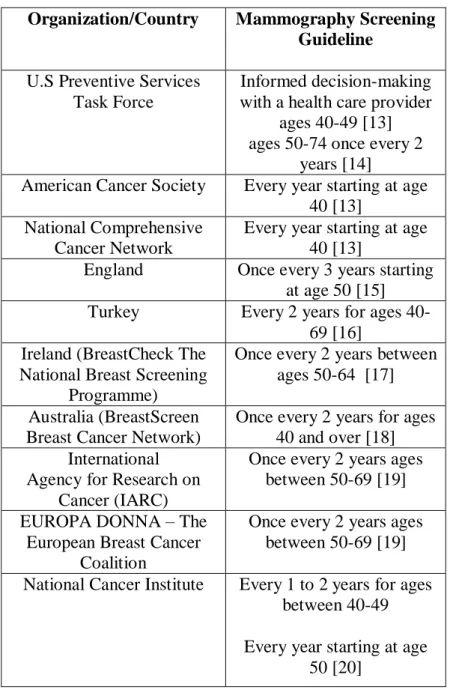
Table 1: Some Mammographic Screening Guidelines for Women at Average Risk ... 5
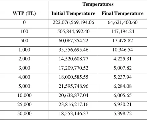
Table 2: Temperature Values Used for SA with Different WTP Values... 42
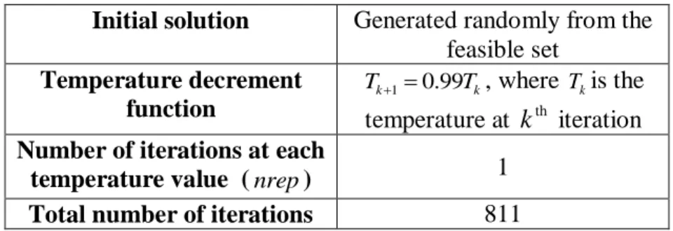
Table 3: Other SA Inputs ... 43
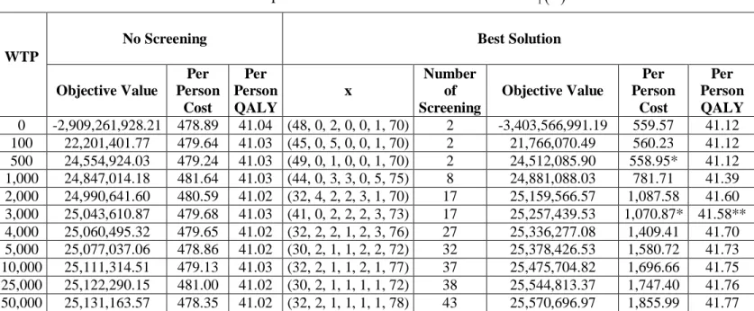
Table 4: Computational Results of Pure SA with NBH x1( ) ... 45
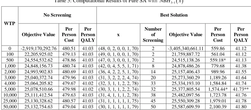
Table 5: Computational Results of Pure SA with NBH3 1
x ... 46Table 6: Computational Results of Pure SA with NBH x3( ) ... 47
Table 7: Computational Results of Pure SA with NBH x5( ) ... 48
Table 8: Computational Results of Reduced VNS with SA... 49
Table 9: Computational Results of Random Search ... 50
Table 10: Best Results Found by the Methods When WTP is 0 TL... 51
Table 11: Best Results Found by the Methods When WTP is 100 TL ... 52
Table 12: Best Results Found by the Methods When WTP is 500 TL ... 53
Table 13: Best Results Found by the Methods When WTP is 1,000 TL ... 54
Table 14: Best Results Found by the Methods When WTP is 2,000 TL ... 55
Table 15: Best Results Found by the Methods When WTP is 3,000 TL ... 56
Table 16: Best Results Found by the Methods When WTP is 4,000 TL ... 57
Table 17: Best Results Found by the Methods When WTP is 5,000 TL ... 58
Table 18: Best Results Found by the Methods When WTP is 10,000 TL ... 59
Table 19: Best Results Found by the Methods When WTP is 25,000 TL ... 60
Table 20: Best Results Found by the Methods When WTP is 50,000 TL ... 61
Table 21: Summary of Best Solutions for each WTP Value... 62
Table 22: Screening Policy in Turkey for Different WTP Values ... 63
Table 23: Comparison Between Recommended Policy and the Best Solutions Found by the Methods ... 64
1
Chapter 1
Introduction
Breast cancer is a potentially dangerous tumor generated from breast cells [1]. Common breast cancer symptoms and signs can be listed as follows:
A newlumpor mass
Swelling of all or part of a breast
Skin irritation or dimpling
Breast or nipple pain
Nipple retraction
Redness, scaliness, or thickening of the nipple or breast skin
Nipple discharge
Swollen lymph nodes[2]
Considering all types of cancers, breast cancer is the most common cancer type among women in the world. Some established risk factors of breast cancer among women are presented in Figure 1.
2
Figure 1: Factors Increasing the Risk of Breast Cancer (reproduced from [3])
1.7 million women were diagnosed with breast cancer and there were 522,000 breast cancer deaths among women in 2012. Furthermore, 6.3 million women were diagnosed with breast cancer between 2007 - 2012 and 25% of cancers in women are breast cancer [4].
Incidence and prevalence rates have increased dramatically (three times) in the last decades in Turkey [5]. Incidence is a measure of new cases arising in a population over a given period. Prevalence is the proportion of actual population found to have a
Factors
Increasing
the
Risk of
Breast
Cancer
Getting olderFamily history of breast cancer Having abnormal genes
Personal history of breast cancer
Being exposed to radiation to chest or face before the age 30 Certain breast changes
Being white Being overweight
Not having a full-term pregnancy Having first child after age 30 Starting menstruating at the age 12 Going through menopause after age 55 Using hormone replacement therapy Drinking alcohol
Having dense breast Smoking
3
condition. It is calculated by comparing the number of people having the same condition with the total number of people studied.
The extent of cancer in the body affects the stage of cancer. The cancer stage is determined considering the following: cancer being invasive or not, size of the tumor, number of lymph nodes affected and whether the cancer is spread to other parts of the body or not. The stage of the cancer has a significant role in prognosis and treatment alternatives. Staging is a process in which how widespread the cancer is at diagnosis is examined. Staging occurs after physical exam, biopsy, chest x-ray, mammograms of breasts, bone scans, computed tomography (CT) scans, magnetic resonance imaging (MRI), and/or positron emission tomography (PET) scans and sometimes blood tests [6]. Stages of breast cancer are numbered from 1 to 4 as explained in Figure 2.
Figure 2: Stages of Breast Cancer (reproduced from [7])
27% of breast cancers is diagnosed in its early stage (stage 1), 53% is diagnosed in stage 2, 9% is diagnosed in stage 3 and 6% is diagnosed in stage 4 [5].
The value of early diagnosis and early detection of breast cancer is presented in studies [8] and [9]. Mammographic screening is proved to be the only screening method that can reduce mortality from breast cancer [10] [11]. Even though mammographic screening has this significant benefit, it is expensive and it can have ramifications such as
Stage 1 •relatively small
cancers
• cancer not spread to the lymph nodes or spread to small area in the sentinel lymph node Stage 2 •larger cancers and/or spread to a few nearby lymph nodes Stage 3 •large tumor (greater than 5 cm) or growing into nearby tissues, or the cancer spread to many nearby lymph nodes Stage 4 •cancer spread
beyond breast and lymph nodes to other parts of the body
4
decreasing life quality and generating false positive results [11]. As a consequence, recommending an effective and cost-efficient mammographic screening policy has high importance.
Recommendations for women to have mammographic screening vary across countries and organizations. These recommendations differ in the age at which the screening should start and how frequent it should be performed among women at average risk for having breast cancer. Table 1 demonstrates some of these screening guidelines for women with average risk. Average-risk women satisfy the following conditions:
having no symptoms
having no history of invasive breast cancer
having no family history in a first-degree relative, or no suggestion/evidence of hereditary syndrome
no history of mantle radiation [12]
5
Table 1: Some Mammographic Screening Guidelines for Women at Average Risk
Organization/Country Mammography Screening Guideline
U.S Preventive Services Task Force
Informed decision-making with a health care provider
ages 40-49 [13] ages 50-74 once every 2
years [14]
American Cancer Society Every year starting at age 40 [13]
National Comprehensive Cancer Network
Every year starting at age 40 [13]
England Once every 3 years starting at age 50 [15] Turkey Every 2 years for ages
40-69 [16] Ireland (BreastCheck The
National Breast Screening Programme)
Once every 2 years between ages 50-64 [17] Australia (BreastScreen
Breast Cancer Network)
Once every 2 years for ages 40 and over [18] International
Agency for Research on Cancer (IARC)
Once every 2 years ages between 50-69 [19] EUROPA DONNA – The
European Breast Cancer Coalition
Once every 2 years ages between 50-69 [19] National Cancer Institute Every 1 to 2 years for ages
between 40-49 Every year starting at age
50 [20]
As it can be understood from Table 1, recommending a screening guideline is a controversial issue in which a global consensus has not been achieved.
6
Turkey also has a guideline which recommends screening once every 2 years for ages 40-69 [16]. However, this guideline is not followed by Turkish women and there is no legal consequence to avoid this situation. Because of that, the effectiveness in terms of life years gained from screening and cost of screening to Turkish women can be questionable. The aim of this study is to find an optimal or near optimal policy that suits Turkish women at average-risk considering the life years gained by screening and the total cost of the policy.
In this study, a mammographic screening policy consists of the following information:
starting age of screening
ending age of screening
screening frequencies for every decade of woman's life until she becomes 80.
The main reason for single/double frequencies recommended in Table 1 is to make the guideline easily memorable among women. However, benefits of mammographic screening vary by age. Considering this, screening frequencies are defined differently for every decade in this study. By having different frequencies, these benefits are aimed to be maximized.
The purpose of this study is to obtain an optimal or near optimal policy in terms of life years gained and cost for Turkish women using Simulated Annealing (SA). Furthermore, this study aims to demonstrate the outcomes in terms of effectiveness and cost when different combinations of policy variables are used. These outcomes can be significant to policy makers. SA is chosen to be the optimization tool because it is widely used in simulation optimization applications. This study utilizes Ada’s Breast Cancer Simulation Model [21] in SA. Ada’s model starts simulating a cohort of cancer-free women when they become 30 until they become 100 or they die. Ada's model is used to run screening policies for Turkish women between ages 30-79 in this cohort. Literature, SEER databases [76], World Health Organization [77], the Ministry of Health of Turkey [78],
7
Turkish Institute of Statistics [78] and heath record systems of Cancer Early Diagnosis and Treatment Centers [80] are the sources of input data [21].
8
Chapter 2
Literature Review about Simulation
Optimization
Simulation model is a mathematical model of a system constructed using simulation. By executing the simulation model, the impact of input variables on the system can be assessed [22].
With enhancements in computer technology, simulation is gaining an important role as a decision making tool. Most of the systems in real world are complicated and because of that obtaining optimal values of the decision variables analytically can be highly challenging. Simulation is a common tool to evaluate and optimize such systems [23], [24]. Simulation optimization refers to the process of finding the best input variable values without explicitly evaluating all possible values [22].
The objective function of a simulation optimization problem with respect to its constraints is as follows: (max) min ( ), X H X (1)
9
Where ( )H X E L X[ ( , )] is the performance measure,L X( , ) is the sample performance. represents the stochastic effects in the system. X denotes a p-vector of controllable factors and denotes the constraint set on the p-dimensional vector of controllable factors. E L X[ ( , )] denotes the expected value of the sample performance. The problem has a single objective if H X( ) is a one-dimensional vector. Otherwise, the problem is multi-objective [24].
Simulation optimization can be classified into two main categories: local optimization and global optimization [24]. Figure 3 demonstrates this classification structure.
10
Figure 3: Classification Structure for Simulation Optimization Problems (adapted from [24])
This study aims to find an optimal or near optimal solution for breast cancer screening for Turkish women. Because of this goal, SA, a global search algorithm is utilized. Due
Optimization Problems Local Optimization Discrete Decision Space Ranking and Selection Multiple Comparison Ordinal Optimization Random Search Simplex/Complex Search Single Factor Method Hooke-Jeeves Pattern Search Continuous Decision Space Response Surface Methodology Finite Difference Estimates Perturbation Analysis Frequency Domain Analysis Likelihood Ratio Estimates Stochastic Approximation Global Optimization Evolutionary Algorithms Tabu Search Simulated Annealing Bayesian/Sampling Algorithms Gradient Surface Method
11
to this, the literature overview in this chapter gives more attention to global optimization techniques.
2.1 Local Optimization
Local optimization can be applied to problems with discrete decision space (finite parameter space and infinite parameter space) and continuous decision space. Most frequently used methodologies for finite case problems are ranking-and-selection and multiple comparison methods. As indicated in [24], Bechhofer et al. [90] and Goldsman and Nelson [91] review these methodologies. Random Search [92] [93] [94], Nelder-Mead Simplex/Complex Search [95], Single Factor Method [96], Hooke-Jeeves Pattern Search [97] can be used for cases considering infinite parameter space. Fu [25] evaluates the use of simulation in optimization of stochastic discrete-event systems by focusing more on the continuous parameter case such as gradient-based methods including perturbation analysis [98], and frequency domain analysis [99].
2.2 Global Search Methods
2.2.1 Evolutionary Algorithms (EAs)
EAs benefit from ideas related to the evolution process. EAs study set of solutions in a way that bad solutions become extinct and good solutions go through evolution in order to obtain an optimal solution. EAs do not need limiting assumptions or knowledge on the shape of the response surface. Because of this advantage, it is a frequently used method for simulation optimization [24]. Possible usages of EAs in the field of simulation optimization and their comparison with the local optimization methods can be found in [24]. The general EA steps used for simulation optimization are as follows. Firstly, a population of solutions is created. Secondly, these solutions are assessed using the simulation model. Then, new solutions are obtained by performing selection and applying genetic operators. New solutions are added to the population. These steps are repeated until the stopping condition is met.
12
Genetic Algorithms (GAs) [26], Evolutionary Programming (EP) [27] and Evolutionary Strategies (ES) [28] are the most commonly used EAs in the literature. The difference between these algorithms can be listed as demonstration of individuals, the creation of variation of operators, and the choice of their reproduction mechanisms. Reviews of the EAs in terms of purpose, structure and working principles can be found in [24]. Detailed evaluations of several techniques used in applying GAs are provided in Liepins and Hillard [29], Davis [30] and Muhlebein [31].
Simulation optimization using EP and ES are not common in literature. However, GAs have received attention for the optimization of complex systems due to their robustness in searching complex spaces and their suitability for combinatorial problems [22] [24]. Works related to simulation optimization using GAs can be found in Bowden and Bullington [32], Dengiz et al. [33], Azadivar and Tomkins [34], Dümmer [35], Wellman and Gemmill [36], McHaney [37], Lee et al. [38], Fontalini et al. [39], Suresh et al. [40].
2.2.2 Simulated Annealing (SA)
SA is proposed by Kirkpatrick et al. [41] and Černý [42]. The algorithm begins with an initial solution which is generally generated randomly. Using a neighborhood structure, a neighbor of this initial solution is obtained. The objective function value of the neighbor solution is calculated. If this solution leads to a better objective function value, then this solution becomes the current solution. If it does not, the neighbor solution is accepted with some probability in order not to get stuck on a local optimum. This acceptance function (i.e., exp
C/Tk
where C represents the difference of objective function value between the current and neighbor solution and Tk is the temperature at k iteration) is calculated. The probability of accepting a worse solution th is less than the value of acceptance function value. T0 is set a high value and it stays the same for a number of iterations and it is gradually decremented until a final temperature is obtained. The initial and final temperatures and the number of iterations at each13
temperature have to be determined a priori in order to apply the SA algorithm [24]. This algorithm is explained in detail in Chapter 4.
Van Laarhoven and Aarts [43], Johnson et al. [44], Eglese [45] and Koulamas et al. [46] evaluates the theory and presents SA applications. Collins et al. [47], Hajek [48] and Fleisher [49] demonstrate several cooling schedules. General working principles of SA algorithms are also explored. Haddock and Mittenthal [50] show that better solutions can be obtained using lower final temperature, slower cooling schedule and more iterations at each temperature. Catoni [51] creates finite-time estimates for cooling schedules. Alkhamis et al. [52] implement Monte Carlo simulation to find objective function value to a stochastic optimization problem using SA. They conclude that modified SA converges with probability of one to an optimal solution given that random error fulfils some conditions. Alrefaei and Andradottir [53] present a SA algorithm with a fixed temperature. They implement two approaches in order to estimate an optimal solution. They demonstrate that these approaches converge to the set of global optimal solutions.
Bulgak and Sanders [54], Gelfand and Mitter [55], Gutjahr and Pflug [56], Fox and Heine [57], and Alrefaei and Andradottir [53] come up with heuristic SA methods for discrete simulation optimization applications.
Yücesan and Jacobson [58] apply local search procedure and five different variations of the SA algorithm to the problem of accessibility of states in a simulation model. They conclude that SA with modified annealing schedule specific to the problem performs better than local search.
Works on optimizing manufacturing systems using SA algorithms are common in the literature. Manz et al. [59] study automated manufacturing system by applying SA algorithm. Brady and McGarvey [60] work on optimizing employee schedules in a pharmaceutical manufacturing laboratory using SA, Tabu Search, GA and a
frequency-14
based heuristic. Baretto et al. [61] study steelworks simulation model based on SA by implementing a version of the Linear Move and Exchange Move (LEO) optimization algorithm.
Zeng and Wu [62] combine perturbation analysis techniques with SA for simulation optimization purposes. Andradottir [63] creates a version of SA for discrete-event simulation optimization. He demonstrates its convergence to a global optimal solution when some conditions are satisfied.
Fu et al. [64] review main simulation optimization approaches, algorithmic and theoretical developments. They conclude that SA applications are successful in simulation optimization. Azadivar [65] studies the optimization of complex stochastic systems using simulation optimization and concludes that SA shows promise in application of simulation optimization.
2.2.3 Tabu Search
Tabu search is a search procedure with constraints. A subset of solution space is eliminated from the search space at each step. As the algorithm goes on, this subset which is constructed by the previous solutions differs [66] [24].
Hu [67] indicates that tabu search performs better than random search and GA for some problems using some standard test functions.
Tabu search is used for simulation optimization. Garcia and Bolivar [68] work on optimization of the simulation model of stochastic inventory with different demand and lead time probability distributions using tabu search. Lutz et al. [69] apply tabu search to optimize the location of buffer and size of the storage in a manufacturing line. Martin et al. [70] work on finding an optimal number of kanbans and lot sizes by implementing versions of tabu search. They show that same outputs can be obtained with less computational time. They indicate that their algorithm can be utilized to find optimal or
15
near-optimal solutions for different industrial problems. Dengiz and Alabas [71] seek an optimal number of kanbans by optimizing the simulation model of a just-in-time system using tabu search. Their results show that tabu search leads to better results than random search.
2.2.4 Bayesian/Sampling Algorithms
In Bayesian/Sampling methodology, the next point is selected in a way that it maximizes the probability of not surpassing the previous point’s value by some positive constant (n) at each iteration [24].
This technique finds points in locations in which the mean performance of the simulation is low for a minimization problem. At the beginning, nhas a small value but it increases as the optimization search gets more local in order the algorithm to converge more rapidly. [24]. Applications of this method for multi-dimensional solution spaces can be found in Lorenzen [72] and Easom [73]. Stuckman and Easom [74] present an overview of existing Bayesian/Sampling methods, such as methods developed by Stuckman [100], Mockus [101], Perttunen [102], Zilinskas [103] and Shaltenis [104]. They also provide comparisons of these methods with methods such as clustering algorithm, SA algorithm and Monte Carlo method. They use a number of test functions with continuous variables. SA in this study has Boltzmann distribution with a constant search radius and a logarithmic annealing schedule. Monte Carlo and SA outperform Bayesian/Sampling methods in terms of computation time. However, they do not perform well in terms of convergence.
2.2.5 Gradient Surface Method (GSM)
GSM is offered by Ho et al. [75] for optimization of discrete-event dynamic systems. GSM uses local search methods to globally investigate a response surface. Considering
16
this, GSM is different from other global search methods. It uses both RSM and efficient derivative estimation techniques and stochastic approximation algorithms [24].
GSM is classified as a global search algorithm since it benefits from information gathered from all solutions in each iteration. Advantageously, a single run is enough for the algorithm to generate gradient estimates. GSM senses the proximity of an optimal solution because of its global orientation [24]. Ho et al. [75] address queuing networks by implementing this algorithm.
17
Chapter 3
Ada’s Breast Cancer Simulation Model
Ada’s simulation model tracks a cohort of cancer-free women at the age of 30 in 2010. The simulation keeps track of a woman until she reaches the age of 100 or she dies. Model inputs are taken from the literature, from the databases of SEER [76], World Health Organization [77], the Ministry of Health of Turkey [78], Turkish Institute of Statistics [79] and from the health record systems of Cancer Early Diagnoses and Treatment Centers [80]. The aim of Ada’s simulation model is to assess and compare the outputs of some breast cancer screening policies (79 annual, 79 biennial, 30-79 triennial, 40-69 annual etc.) [21].Flowchart of the model is presented in Figure 4. The flow of a single entity, which is women, is as follows. At the beginning of the simulation, cancer-free 30 year old women in 2010 are created. The attributes such as age, life status (being dead or alive), and cancer stages are assigned. There are two ways for breast cancer detection, mammography screening and clinical breast examination [21].
With some death probability estimated using the data from Turkish Institute of Statistics [79] for 2000 - 2010, the woman dies because of non-breast cancer related reasons. The
18
woman is either disposed from the model because of non-breast cancer related death or with some probability she is sent to clinical breast examination. An abnormal finding in clinical diagnosis results in sending the woman to treatment [21].
When no such finding occurs or clinical breast examination is not required, the woman is re-sent to the mammography screening considering the mammography screening policy. If she goes through screening and gets a positive result, this means that an abnormal result is obtained and she is sent to treatment. Under the case of no screening or she gets a negative screening result, her tumor progresses. Tumor progress means that the woman’s cancer status changes. Tumor progresses according to a Markov Chain. The Markov Chain of Fryback et al. [81] is taken as an initial data and it is modified in order to cover the situation in Turkey. If the woman is diagnosed with a breast cancer, her stage of the disease may stay the same or it can progress to a later stage or she may die. If the woman is not diagnosed with a breast cancer, she may stay healthy or she may have a breast cancer later [21].
The woman who is sent to treatment is removed from the system because of breast cancer or other reasons [21].
At the end of each year, each entity’s age attribute is increased by one and the following counters are calculated: total incidence rates for each year, incidence by stage for each year, breast cancer mortality rates, other causes mortality rates, the number of mammograms for each year, the number of true positive and false positive results for mammography, the number of clinical diagnosis, total life year for each year, Quality adjusted life years (QALY) for the corresponding year, and total cost for each year. Total cost includes screening cost, treatment cost and false positive cost [21].
The objective function consists of QALYs and total cost. Ten replications are performed and their average values of QALY and total cost are used to calculate the objective value of each policy in SA.
19
20
Chapter 4
Simulated Annealing (SA)
SA is similar to metallurgical annealing. Metallurgical annealing involves heating the metal and cooling it off slowly so that the crystals get larger and the defects decrease at the same time. Atoms are dissolved out from their initial positions by the heat. This can be considered as energy level’s local optimum. These atoms have the ability to move freely. They can locate in places with lower energy levels than their previous places due to slowly cooling off. Choosing appropriate cooling procedure is important because cooling off too fast can result in atoms not finding better energy levels and cooling off too slow can take a lot of time [82].
SA is a robust and general metaheuristics method capable to find global optimum because it can avoid getting stuck in local optima and it can remember the best objective value obtained from iterations performed [83]. It is demonstrated that when some conditions are hold SA converges with probability of one to a global optimal solution [82].
Constructing exact solution methods can be challenging for some optimization problems. For example, for cases in which no exact solution method are applicable or
21
applying exact solution methods are computationally complicated or information about the problem are not enough to build an existing model. For those cases, SA can be highly beneficial [84]. SA can also be applied to problems involving nonlinear models, disorganized and noisy inputs and problems with numerous constraints [83]. A mathematical model is not necessary to implement SA. Being able to design a solution in a way that it can be perturbed and evaluated is enough to use SA to solve the optimization problem [84].
SA is independent of any restrictive features of the model. Because of that it is more flexible than the local search methods. Therefore, tuning SA to enhance its performance takes less effort than tuning local search methods. To tune local search methods, being familiar with the code is required which takes time and effort [83].
Because of the above advantages, SA is evaluated to be a promising [65], successful [64] and frequently used heuristic method for simulation optimization [22]. Some studies in which SA is applied for simulation optimization is as follows: Bulgak and Sanders [54], Haddock and Mittenthal [50], Gelfand and Mitter [55], Gutjahr and Pflug [56], Fox and Heine [57], and Alrefaei and Andradottir [53], Eglese [45], Andradottir [63], Yücesan Jacobson [58], Manz et al. [59].
Because of its advantages, its frequent usage in simulation optimization and its premise, SA is chosen to be the solution method in this study.
In all iterations, SA compares the objective function value of the current solution with the objective function value of the newly generated solution. SA moves to the newly generated solution with better objective function value (improving move). It also moves to newly generated solution with worse objective function value (non-improving move) with a probability. It performs these non-improving moves in order to go away from local optimal solutions. The SA algorithm for the maximization case is presented as Algorithm 1.
22
Here, X denotes the feasible solution set, xnow is the previously accepted solution (current solution). T0 represents the initial temperature, iteration count counts the number of iterations performed by the algorithm. nrep is the number of iterations performed at each temperature.T denotes the final temperature which is set at the f beginning of the algorithm. The temperature reduction function is Tk k1Tk1 where
(0,1) k
is the temperature decrement rate. xbest is the solution with the best objective value found so far.Objective function x( ) is the function utilized to calculate the objective function value of the corresponding solution. N x( now) is the neighborhood of the current solution andxnext is the solution obtained from the neighborhood of the current solution. C denotes the difference between the objective function values of the current and next solution.
23 Algorithm 1 SA for Maximization
0
Step 1: Initialization
1.1 Choose an initial solution
1.2 Choose an initial temperature 0
Set 0 and 0
Set 0 and final temperature Choose a temperat now f x X T iteration count k nrep T 1 1 1 1
ure reduction function ( ) 1.3
Step 2: Choice and Termination
2.1 If , then set 1,
reduce the temperature ( ) and set 0
2.2 k k k best now k k k T T x x
iteration count nrep k k
T T iteration count
Terminate when , return
2.3 If , increase by one
Randomly choose from ( )
Set ( ) - ( ) 2.4 If 0 proceed k f best k f next now now next T T x T T iteration count x N x
C objective function x objective function x C
to Step 3 (Accepted)
Else, generate uniformly in the range (0,1)
2.5 If exp(- / ) then proceed to Step 3 (Accepted) Else proceed to Step 2.1 (Rejected)
Step 3: Update 3.1 Set k now next R R C T x x If ( ) ( ) 3.2 Go to Step 2 now best best now
objective function x objective function x
x x
The temperature parameter has a significant role on the probability of accepting non-improving moves [82].
24 4.1 Representation of a Policy and Feasible Policies
The solution consists of 7 components, which arex x x x x x x1, 2, 3, 4, 5, 6, 7. x1 represents the starting screening age. It is an integer between 30 and 49 (30 and 49 are included). x2 represents the frequency of screening when the woman is in her 30s. x3 represents the frequency of screening when the woman is in her 40s. x4 represents the frequency of screening when the woman is in her 50s. x5 represents the frequency of screening when the woman is in her 60s. x x x x2, 3, 4, 5 are integers between 0 and 5 (0 and 5 are included). x6 represents the frequency of screening when the woman is in her 70s. x6 is an integer between 1 and 5. x7 is the stopping screening age. It is between 70 and 79 (70 and 79 are included).
For example, the following solution x
30,5, 0,5, 4,1, 71
corresponds to screening at the following ages: 30, 35, 50, 55, 60, 64, 68, 70 and 71.The possible starting and ending screening ages are chosen as above because Ada’s Breast Cancer Simulation Model uses data compatible with these ages. The screening frequencies are chosen dynamically as above to include most of the possible combinations.
All combinations of x x x x x x x1, 2, 3, 4, 5, 6, 7 are not feasible because there are intuitive connections between x x x1, 2, 3 andx x6, 7. For example x
30, 0,1,1,1,1, 70
is not feasible because if starting age is 30, then there should be at least one screening between ages 30 to 39. However, in this solution the screening frequency for 30s is given as 0.The feasible solution set X is the set of x( ,x x x x x x x1 2, 3, 4, 5, 6, 7) vectors satisfying the following conditions:
25 1 1 1 1 2 1 1 {30,31,32,33,34,35,36,37,38,39, 40, 41, 42, 43, 44, 45, 46, 47, 48, 49} {0} 40 {1} 39 {1, 2} 38 {1, 2,3} 37 {1, 2,3, 4} 36 x if x if x if x x if x if x 1 1 1 1 3 1 1 {1, 2,3, 4,5} 35 {1} 49 {1, 2} 48 {1, 2,3} 47 {1, 2,3, 4} 46 {1, 2,3, 4,5} 40 45 {0,1, 2,3, 4,5} if x if x if x if x x if x if x if 1 4 5 7 7 7 6 7 39 {0,1, 2,3, 4,5} {0,1, 2,3, 4,5} {1} {70, 71, 77} {1, 2} 72 {1,3} {73, 79} {1, 2, 4} {74, 78} {1,5} x x x if x if x if x x if x if 7 7 7 75 {1, 2,3} 76 {70, 71, 72, 73, 74, 75, 76, 77, 78, 79} x if x x
26
The quality of the initial solution has an impact on the performance of the SA algorithm [82]. To reduce this dependency, initial solutions are randomly generated from the feasible set.
4.2 Parameters of SA Algorithm
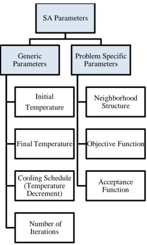
Parameters of SA can be categorized as generic parameters and problem specific parameters as presented in Figure 5. Generic parameters include initial temperature, final temperature, cooling schedule and number of iterations. Problem specific parameters are neighborhood structure, objective function and acceptance function. Literature on these parameters and their choices in this study are explained in this section.
Figure 5: Parameters of SA Algorithm SA Parameters Generic Parameters Initial Temperature Final Temperature Cooling Schedule (Temperature Decrement) Number of Iterations Problem Specific Parameters Neighborhood Structure Objective Function Acceptance Function
27
Several combinations with different initial and final temperatures, cooling schedules and number of iterations at temperatures can be tried to choose good parameter settings. However, for practical applications, this may not be possible [85]. The approaches applied in literature to choose generic parameters are reviewed in the following section.
4.2.1 Generic Parameters
A schedule resulting in near optimal solutions within reasonable computation time can be found in [85]. The initial temperature T0 and the temperature decrement
k between the temperatures Tk and Tk1. Tkis the temperature at kth iteration and Tk1 is the temperature at (k+1)st iterations. Tk and Tk1 are chosen considering the mean value c and standard deviation of the cost function using equations in (2).0 1 exp ( ) k k k k k k T c T T T T (2)
The starting temperature T0 is chosen in a way that makes the probability of accepting a solution in the interval of [ - 3 ,c c3 ] high. (0,1] effects the speed of temperature decrease. It is found out that0.7 is a good choice [85].
Alrefaei and Diabat [86] address a multi-objective inventory problem using SA. Their algorithm uses constant temperature and it accepts a solution according to their rule. This rule is related to the estimated objective function values.
Manz et al. [59] focuses on an automated manufacturing system for assembling of three products. Several values of initial and final temperatures, temperature decrements and number of iterations at each temperature are combined and assessed.
28
Uhlig and Rose [87] introduce an approach to create schedules for tool groups in semiconductor manufacturing using SA. They begin with a very high temperature and perform many iterations. The temperature decrement () is chosen in a way that the final temperature is nearly 0.
A more complicated way uses certain desired acceptance probabilities. P is the probability of accepting objective function value ( C ) difference.
( , ) exp ln( ) C C P C T T T P (3)
Then, (3) can be used to define initial temperature, T0 and temperature value at kth iteration Tk in the annealing schedule. Standard deviation of a sample of random solutions can be used to make estimations for possible difference values. After defining these two temperature values, the whole schedule can be obtained by using (4) [87].
(1/ k) 0 k k T T (4)
Busetti [83] chooses an initial temperature T0 in a way that there is an 80% chance that a worse solution is accepted. He suggests doing an initial search in which all worse solutions are accepted in order to come up with an estimate of T0 and then calculating the average objective difference observed (C).p0is the initial acceptance probability.
0 T is then calculated by (5). 0 0 ln( ) C T p (5)
29
An empirical rule is suggested to find an initial temperature T0 and perform some transitions. The rule is to multiply the T0by 2 and perform the same procedure as long as (6) is less than a previously defined w0 value.
number of accepted transitions number of proposed transitions
w (6)
(6) is referred as the acceptance ratio. Kirkpatrick et al. [105] take w0 as 0.8 [88]. This rule is adopted in some studies with a few modifications. T0 can be set by observing the average change in objective function value (C) of numerous random solutions and using (6) to find w0 for a minimization problem and using (7) for T0.
( )
C
denotes the positive difference of objective values [88].
0 ( ) 0 exp C w c (7) ( ) 0 0 ln(w 1) C T (8)
As indicated in [88], similar formula are used in works of Leong et al. [106] [107], Skiscim and Golden [108] [109], Morgenstern and Shapiro [110], Aarts and Van Laarhoven [111], Lundy and Mees [112], and Otten and Van Ginneken [113].
Bulgak and Sanders [54] generate a discrete event simulation model to search for an optimal buffer sizes for a manufacturing system. Their SA algorithm stops after reaching a maximum number of solutions generated.
Apart from setting a final temperature and executing the algorithm until it reaches this temperature, one can terminate the execution when amount of improvements decrease. Lack of improvement can be defined as no improvement (no new best solution at one
30
temperature) and/or the acceptance ratio falling below defined value [83]. The algorithm can stop when the best objective function value fails to improve by at least a defined percent after some number of cool offs. Another stopping condition can be to end the algorithm when the number of accepted moves in some predefined number of temperature decreases is less than a defined percent [82].
The temperature decrement can change the ability of SA to converge to the global optimum. This convergence is proven when there is a logarithmic temperature decrement. A low cooling rate may result in an increase in computation time, whereas a high cooling rate may lead to getting stuck in a local optimum [82].
Nahar et al. [114] fix the number of temperature decrement steps into K and they choose T kk, 1 K, the corresponding temperature values. They use 6 temperature values [88].
Skiscim and Golden [108] [109] split the interval
0,T0
into a constant number of K subintervals and Tk is chosen using (9).
0 , 1, , k K k T k K KT (9)In Huang et al. [115], the decrement ratio
k is chosen in such a way that the expected mean value of the objective function at Tk1 is in a range of around the attained mean value at Tk [85].The cooling rule presented in (10) was first proposed by Kirkpatrick et al. [105].
31
where is a constant smaller than but close to 1 and takeas 0.95 .
This cooling schedule is also used in other SA applications such as Johnson et al. [116], Bonomi and Lutton [117] [118], Burkard and Rendl [119], Leong et al. [106] [107], Morgenstern and Shapiro [110], and Sechen and Sangiovanni-Vincentelli [120], with values of
ranging from 0.5 to 0.99 [88].As in (3), we set the initial temperature and final temperature using initial acceptance and final acceptance probabilities. Initial acceptance probability is taken as 0.99 and the final acceptance probability is taken as 15
10 . Sample of 100 solutions is considered to
make estimations for objective value difference.
Cooling rule in (10) with 0.99 is used. At each temperature one iteration is performed. As explained in Section 4.2.2.2, objective value consists of Willingness to Pay (WTP) value, which corresponds to extra money that can be paid to gain one QALY. Several WTP values are considered in computational studies. The temperatures are set for each WTP value, separately.
The other abovementioned methods to set generic parameters are tried in the study. The best performance is obtained from the utilized method.
4.2.2 Problem Specific Parameters 4.2.2.1 Neighborhood Structure
Neighborhood structure is an important component of all metaheuristics. In order to define a proper neighborhood structure, efficiency and effectiveness of the neighborhood have to be taken into consideration. Efficiency refers to the quality of neighborhood structure’s performance to cover the feasible solutions. Speed, computational effort and number of neighbors can be significant factors that can have an impact on the efficiency. Effectiveness is the ability of the neighborhood structure to cover feasible solutions [82].
32
Using different neighborhoods in a systematic manner can be useful to avoid getting stuck in local optimal solutions. The Variable Neighborhood Search (VNS) is the only metaheuristic that considers changing neighborhood structures in iterations [82]. VNS is introduced by Hansen and Mladenović [89]. VNS takes increasingly further neighborhood structures into account until a better solution compared to the incumbent solution is found. Benefitting from this structure, some favorable properties of the incumbent solution can be maintained. For example, some variables may already be at their optimal values and this incumbent solution is used to obtain good neighbor solutions [89].
The following facts are used systematically in VNS.
A local minimum of one neighborhood structure may not be a local minimum to another neighborhood structure.
A global minimum is a local minimum for all possible neighborhood structures.
Local minima of one or more neighborhoods are relatively close to each other for several problems [89].
There are some different types of VNS. In this study, we use Reduced VNS which is presented as Algorithm 2.
33
Algorithm 2 Reduced VNS [89]
max
Step 1: Initialization
Choose the set of neighborhood structures , for 1,..., Choose an initial solution
Choose a stopping condition
Step 2: Repeat the following steps until the stopping con i now N i i x max th dition is met 2.1 Set =1
2.2 Repeat the following steps until a. Shaking
Generate a point randomly from the neighborhood of
i i i x i ( ( )) b. Move or not
If this point is better than the incumbent, move there ( ) and continue the sea
now i now now x x N x x x 1
rch with ( 1), otherwise set 1
N i i i
The set of neighborhoods
m
1 , 2 , ,Ni ax x
N x N x regarded around the current point
x are often nested. This means that each neighborhood includes the previous one [89]. Algorithm 2 chooses a point at random in the first neighborhood. If its objective function value is better than that of the incumbent, the search is recentered around x. Otherwise, the algorithm proceeds to the next neighborhood. After considering all neighborhoods, the algorithm returns to the first neighborhood until the stopping condition is achieved [89].
Taking imaxas one in Algorithm 2 corresponds to having a single neighborhood structure, as used in other search heuristics [89].
Upper limit on execution time allowed and upper limit on the number of iterations between two improvements can be possible stopping conditions for Algorithm 2.
34
To prevent getting stuck at a local optimum, taking the union of neighborhoods of any feasible solution x should lead to reaching the whole feasible set. This means that (11) holds.
XN x1( )N x2( ) ... Nimax( ) , x x X (11)
The neighborhood definitions may contain X without partitioning it. Covering X can easily be implemented using nested neighborhoods, satisfying (12) [89].
N x1( )N x2( ) ... Nimax( ) and Xx Nimax( ) , x x X (12)
Considering the above neighborhood structures and the factors affecting the efficiency and effectiveness of the neighborhood, problem specific neighborhood structures are generated. In all neighborhood structures, all neighbor solutions have equal probability to be the next solution. Let the current solution be x
x x x x x x x1, , , , , ,2 3 4 5 6 7
, xX. The neighborhoods of this point according to the structures
ma1 , 3 1 , 3 , 5 , i x( )
NBH x NBH x NBH x NBH x NBH x are presented in (13). The neighborhood definitions are common for the frequencies (i.e.,x x x x x2, 3, 4, 5, 6). The neighbor solution can maintain the current solution’s frequency or it can increase or decrease it by one for each frequency with equal probabilities. The neighbors differ for the starting and stopping ages (i.e., x1 and x7). In NBH x , the neighbor solution can 1
maintain the current solution’s starting age or it can increase or decrease it by one with equal probabilities. The same holds for the stopping age. In NBH3 1
x , the neighbor solution can maintain the current solution’s starting age or it can increase or decrease it by three at maximum with equal probabilities. The neighbor solution can maintain the current solution’s stopping age or it can increase or decrease it by one with equal probabilities. In NBH5
x the neighbor solution can maintain the current solution’s starting age or it can increase or decrease it by five years at maximum with equal35 probabilities. The same holds for the stopping age.
max( )
i
NBH x is defined as the entire feasible set, X .
1 1 2 3 4 5 6 7 1 1 1 2 2 2 3 3 3 4 4 4 5 5 5 6 6 6 7 7 7 { =( , , , , , , ) : 1, 1 , 1, 1 , 1, 1 , 1, 1 , 1, 1 , 1, 1 , 1, 1 , = NBH x x x x x x x x x x x x x x x x x x x x x x x x x x x x x x x X }
3 1 1 2 3 4 5 6 7 1 1 1 2 2 2 3 3 3 4 4 4 5 5 5 { ( , , , , , , ), 3, 3 , 1, 1 , 1, 1 , 1, 1 , 1, 1 , NBH x x x x x x x x x x x x x x x x x x x x x x x x
6 6 6 7 7 7 x x 1,x 1 , x x 1,x 1 , xX} (13)
1 2 3 4 5 6 7 1 1 1 2 2 2 3 3 3 4 4 4 5 5 5 6 6 6 7 7 7 3 { = , , , , , , }, 3, 3 , 1, 1 , 1, 1 , 1, 1 , 1, 1 , 1, 1 , 3, 3 , } { NBH x x x x x x x x x x x x x x x x x x x x x x x x x x x x x x x X
1 2 3 4 5 6 7 1 1 1 2 2 2 3 3 3 4 4 4 5 5 5 6 6 6 7 7 7 5 { = , , , , , , }, 5, 5 , 1, 1 , 1, 1 , 1, 1 , 1, 1 , 1, 1 , 5, 5 , } { NBH x x x x x x x x x x x x x x x x x x x x x x x x x x x x x x x X max( ) i NBH x XThese neighborhoods are nested, satisfying (14).
max
1 3 1 3 5 i ( )
NBH x NBH x NBH x NBH x NBH x X
36 4.2.2.2 Objective Function
SA compares the objective function value of the current solution and a newly created solution and then makes the move. Simulation model can be used to obtain the objective function value [34].
The objective function used in this study is constructed from Ada’s Breast Cancer Simulation Model’s outputs. QALY is a measure to evaluate the benefits of healthcare interventions. It is based on number of years of life that would be added if the healthcare intervention is done. Using some Willingness to Pay (WTP) values, total cost is converted into QALY in order to have a single objective which is in terms of life years. WTP represents the amount of money that can be spent in order to gain a QALY.
At each iteration (15) is calculated for the newly generated solution.
2080 2080 2010 2010 maximize i i i i Total Cost QALY WTP
(15) The objective function, presented in (15) consists of three components. QALY, total costand WTP. The calculation of QALY and total cost are presented in Ada [21]. QALY and total cost values are added for years 2010 - 2080 for the women who were born in 1980. These women become 30 in 2010 and since the starting screening age is between 30 and 49 (30 and 49 are included), the summation begins from 2010. WTP value is not fixed. Because of that eleven different WTP values are used in SA. These are 0 TL; 100 TL; 500 TL; 1,000TL; 2,000 TL; 3,000 TL; 4,000 TL; 5,000 TL; 10,000 TL; 25,000TL and 5,0000 TL. The objective function is in terms of QALY, so the objective is to maximize this value.
37 4.2.2.3 Acceptance Function
SA accepts worse solutions considering the acceptance function. Because of that it has an important role to obtain better solutions [82]. The acceptance function used in this study is offered by Kirkpatrick et al. [41] and it is presented in (16).
Rexp
C T/ k
(16) R is a uniformly generated number and R(0,1). C is the objective functiondifference between the current and the newly generated solution. is the temperature value at kth iteration. If the objective function value of the new solution is worse than the current solution. SA generates aRvalue and checks (16). If it holds, then the worse solution is accepted [68]. In this study, approximation of acceptance function proposed by Johnson et al. [121], presented in (17), is used. Johnson et al. [121] found that acceptance calculation take nearly one third of the computation time. This approximation is useful in terms reducing computation time.
R 1
C/Tk
(17) 4.3 Applied Methods Using SAWith the parameter selections presented in Section 4.2, SA algorithm is applied in the following methods. Pure SA, presented as Algorithm 1, with
1 , 3 1 , 3 ,
NBH x NBH x NBH x and N HB 5
x ,NBHimax( )x neighborhood structures.SA can be combined with the Reduced VNS heuristic. Reduced VNS with SA is presented as Algorithm 3.
k
38 Algorithm 3 Reduced VNS with SA
0
Step 1: Initialization
1.1 Choose an initial solution
1.2 Choose an initial temperature 0
Set 0 and 0
Set 0 and final temperature Choose a temperat now f x X T iteration count k nrep T 1 1 max
ure reduction function 1.3
1.4 Choose the set of neighborhood structures , for 1,..., Step 2: Choice and Termination
2.1 Set =1
2.2 Repeat the following steps 2.2.1 If k k k best now i T T x x N i i i iter 1 1 , then set 1,
reduce the temperature ( ) and set 0
2.2.2 Terminate when , return
2.2.3 If , increase by one
Rando
k k k
k f best
k f
ation count nrep k k
T T iteration count T T x T T iteration count
mly choose from ( )
Set ( ) - ( )
2.2.4 If 0 proceed to Step 3 (Accepted) and set 1 Else, generate uniformly in the range (0,1)
2.
next i now
now next
x N x
C objective function x objective function x
C i R max max
2.5 If exp(- / ) then set 1 (if set 1) and proceed to Step 3 (Accepted)
Else set 1 (if set 1) and proceed to Step 2.2.1 (Rejected) Step 3: U k R C T i i i i i i i i i i pdate 3.1 Set If ( ) ( ) 3.2 Go to Step 2 now next now best best now x x
objective function x objective function x
x x xx
39
Like Pure SA, the algorithm begins with setting initial solution, initial temperature and temperature reduction function. In addition to these, the neighbor structures are also defined. Difference between Pure SA and Reduced VNS with SA is that neighborhood structure to be used in the next iteration to find the next solution depends on whether a good solution is reached or not in the current iteration.
The search for next solution begins in the first neighborhood. If the solution gives better result, then the search continues in this neighborhood. If it is not better but if it is accepted, the search continues in the second neighborhood which is larger than the first neighborhood. Performing the search in the second neighborhood also occurs if the solution is rejected.
During the search, moving to a better solution results in narrowing the search region to first neighborhood and finding a worse next solution leads to enlarging the neighborhood by using the next neighborhood structure. When the largest neighborhood is reached, then the search returns to the first neighborhood. This is repeated until the final temperature is larger than the current temperature.
Random Search, presented as Algorithm 4, is also applied in order to assess the performances of Pure SA and Reduced VNS with SA.
40 Algorithm 4 Random Search
Step 1:Initialization
1.1 Choose an initial solution
1.2 Set 0
1.3
Step 2: Repeat the following until reaches a defined number 2.1 Randomly ch now best now x X iteration count x x iteration count oose from Increase by 1 Set ( ) - ( ) 2.2 If 0 proceed to 1.4.3 (Accepted) 2.3 Set If next now next now next x X iteration count
C objective function x objective function x C x x objec ( ) ( ) now best best now
tive function x objective function x
x x
![Figure 2: Stages of Breast Cancer (reproduced from [7])](https://thumb-eu.123doks.com/thumbv2/9libnet/6019299.127045/11.918.173.812.554.758/figure-stages-breast-cancer-reproduced.webp)
![Figure 4: Flow Chart of Ada’s Simulation Model (adapted from [21])](https://thumb-eu.123doks.com/thumbv2/9libnet/6019299.127045/27.918.170.711.227.861/figure-flow-chart-ada-s-simulation-model-adapted.webp)