© Author(s) 2018. This work is distributed under the Creative Commons Attribution 4.0 License.
Carbonaceous material export from Siberian permafrost tracked
across the Arctic Shelf using Raman spectroscopy
Robert B. Sparkes1, Melissa Maher1, Jerome Blewett2,a, Ayça Do˘grul Selver2,3, Örjan Gustafsson4, Igor P. Semiletov5,6,7, and Bart E. van Dongen2
1School of Science and the Environment, Manchester Metropolitan University, Manchester, UK
2School of Earth and Environmental Sciences and Williamson Research Centre for Molecular Environmental Science,
University of Manchester, Manchester, UK
3Balıkesir University, Geological Engineering Department, Balıkesir, Turkey
4Department of Environmental Science and Analytical Chemistry (ACES) and the Bolin Centre for Climate Research,
Stockholm University, Stockholm, Sweden
5Pacific Oceanological Institute Far Eastern Branch of the Russian Academy of Sciences, Vladivostok, Russia 6International Arctic Research Center, University of Alaska, Fairbanks, USA
7National Tomsk Research Polytechnic University, Tomsk, Russia
anow at: Organic Geochemistry Unit, School of Chemistry, Cabot Institute, University of Bristol, Bristol, UK
Correspondence: Robert B. Sparkes ([email protected]) Received: 19 January 2018 – Discussion started: 9 March 2018
Revised: 17 August 2018 – Accepted: 6 September 2018 – Published: 11 October 2018
Abstract. Warming-induced erosion of permafrost from Eastern Siberia mobilises large amounts of organic carbon and delivers it to the East Siberian Arctic Shelf (ESAS). In this study Raman spectroscopy of carbonaceous material (CM) was used to characterise, identify and track the most re-calcitrant fraction of the organic load: 1463 spectra were ob-tained from surface sediments collected across the ESAS and automatically analysed for their Raman peaks. Spectra were classified by their peak areas and widths into disordered, in-termediate, mildly graphitised and highly graphitised groups and the distribution of these classes was investigated across the shelf. Disordered CM was most prevalent in a permafrost core from Kurungnakh Island and from areas known to have high rates of coastal erosion. Sediments from outflows of the Indigirka and Kolyma rivers were generally enriched in inter-mediate CM. These different sediment sources were identi-fied and distinguished along an E–W transect using their Ra-man spectra, showing that sediment is not homogenised on the ESAS. Distal samples, from the ESAS slope, contained greater amounts of highly graphitised CM compared to the rest of the shelf, attributable to degradation or, more likely, winnowing processes offshore. The presence of all four spec-tral classes in distal sediments demonstrates that CM
de-grades much more slowly than lipid biomarkers and other traditional tracers of terrestrial organic matter and shows that alongside degradation of the more labile organic matter com-ponent there is also conservative transport of carbon across the shelf toward the deep ocean. Thus, carbon cycle calcula-tions must consider the nature as well as the amount of car-bon liberated from thawing permafrost and other erosional settings.
1 Introduction
Extensive Northern Hemisphere permafrost deposits contain approximately 40 % of the global soil organic carbon (OC) budget (Schuur et al., 2015; Tarnocai et al., 2009). The ma-jority of this carbon is currently freeze-locked, but rapid warming at high latitudes is making it increasingly vulner-able to mobilisation via fluvial and coastal erosion. Thawing also leads to degradation, both in situ and post-mobilisation, to greenhouse gases, providing a positive feedback response to warming (Stendel and Christensen, 2002; Vonk et al., 2010, 2015). The Eurasian Arctic region contains the major-ity of Northern Hemisphere permafrost OC, and the release
rate of both OC and sediment from this area into the Arc-tic Ocean is predicted to rise during the next century (van Dongen et al., 2008; Holmes et al., 2002, 2012; O’Donnell et al., 2014; Peterson et al., 2002). Deepening hydrologi-cal flow paths and thermokarst erosion events are mobilis-ing “old” carbon that has been stored in deep permafrost for thousands of years (Gustafsson et al., 2011; Feng et al., 2013, 2015; Vonk et al., 2012; Vonk and Gustafsson, 2013; IPCC, 2013). OC delivered by fluvial erosion and transport has been identified offshore using molecular biomarkers and has been shown to deposit and/or degrade rapidly on the shelf (Bröder et al., 2016; Do˘grul Selver et al., 2015; Karlsson et al., 2015; Sparkes et al., 2015, 2016; Tesi et al., 2014, 2016). In ad-dition to fluvial erosion, coastal erosion delivers a significant amount of sediment and OC (44±10 Tg OC yr−1) to the Arc-tic Ocean (Vonk et al., 2012). Poorly lithified coastal cliffs, combined with stormy weather, have caused erosion rates of up to 10 m yr−1(Lantuit et al., 2011). Reducing sea ice cover, and therefore increased wave fetch and storm impact, is also likely to increase coastal erosion rates during the next cen-tury (Feng et al., 2015; Stein and MacDonald, 2004; Vonk et al., 2010).
1.1 Recalcitrant organic matter export from permafrost
Erosion of ancient carbon from Arctic permafrost may lead to degradation of carbon into greenhouse gases and a positive feedback effect on global climate, or the absence of degra-dation may allow this material to be used to track eroded sediment across the continental shelf. Alongside modern OC transport, erosion mobilises petrogenic OC from rocks and soils (also known as carbonaceous material, CM) and deliv-ers this to the ocean. CM consists of recalcitrant material, such as coal, lignite, combustion-derived black carbon, kero-gen (insoluble hydrocarbons; Durand, 1980) and graphite, which is stable over millions of years. CM is (apart from black carbon) formed from the maturation of buried organic matter, with the degree of diagenesis and metamorphism controlling the molecular and crystalline structure (Beyssac et al., 2002b, 2003a, 2007). High temperatures during burial and metamorphism drive the transition from disordered kero-gen and lignite to highly crystalline graphite, allowing CM from different areas to be identified due to differences in the geological history of the source rocks (Sparkes et al., 2013). CM represents a major fraction of the global OC bud-get, sequestered in sedimentary and metamorphic rocks over million-year timescales (Bouchez et al., 2010; Galy et al., 2007; Hilton, 2008; Smith et al., 2013). Any oxidation of CM during erosion, transport and burial represents a movement of carbon between the long-term and short-term carbon cycles. During transport, bioavailability of CM is believed to be low, but there is evidence that extremely long transport distances can degrade disordered CM, leaving only crystalline graphite (Bouchez et al., 2010; Galy et al., 2007). Previous work has
investigated CM in tropical and subtropical settings, but, in contrast to extractable OC, no work has been done to charac-terise or trace CM in the Arctic. The only studies on recalci-trant Arctic OC involve (usually submicron-sized) soot black carbon particles (Coppola et al., 2014; Salvadó et al., 2017; Winiger et al., 2017).
Salvadó et al. (2017) measured the distribution of soot black carbon (SBC) across the ESAS. SBC was isolated us-ing chemothermal oxidation at 375◦C, a method that has been thoroughly tested to isolate combustion-derived SBC from other recalcitrant species (such as coal of various degree of maturity, pollen and other biomacromolecules; Gustafs-son et al., 2001; Elmquist et al., 2006). The highest con-centrations (up to 0.22 wt % SBC) and proportions (11% of the total OC) of SBC were found at the mouths of the Lena and Kolyma rivers, with concentrations and proportions de-creasing offshore as SBC was deposited and marine pri-mary productivity became the dominant OC source. How-ever, the relative importance of the recalcitrant SBC within the permafrost-derived carbon pool increased as more labile material degraded during transport. This pattern was seen consistently along a W–E transect from the Laptev Sea to the Eastern ESAS. The authors concluded that the source of SBC was not atmospheric deposition (e.g. via biomass burn-ing) but permafrost erosion. Goñi et al. (2005) report anoma-lously old radiocarbon ages for distal sediments on the Beau-fort Shelf, attributed to highly recalcitrant terrestrial OC that has been matured to kerogen grade or higher, but the nature and origin of the material has not been investigated in detail. Therefore, there is a need to assess whether the various inputs of carbon to the Arctic Ocean system can explain these old radiocarbon ages, and whether they form an active or passive part of the carbon cycle.
This study uses Raman spectroscopy to identify the sources of CM in the Eastern Siberian region and tracks the export of CM from these sources across the East Siberian Arctic Shelf (ESAS). This is the first Raman study of sedi-mentary CM in the Arctic. Automated Raman spectra fitting procedures were used to analyse > 1400 spectra measured from CM in sediments collected across 1 million km2of the (ESAS). Multiple heterogeneous sources of sediment were studied, including several of the world’s largest river catch-ments and thousands of kilometres of shoreline experiencing rapid coastal erosion (Lantuit et al., 2011).
1.2 Raman spectroscopy
Raman spectroscopy is a precise and powerful tool for quan-tifying the degree of crystallinity within CM (Beyssac et al., 2002a, 2003b). In this study, it is used to identify permafrost-sourced CM offshore. Monochromatic incident light inter-acts with the crystal lattice of the targeted particle and re-flects with a changed wavelength due to the energy shift introduced by lattice vibrations (phonons). When analysed with in a Raman spectrometer, graphitic and disordered
car-bon can be characterised by studying the response within the range of 800–2000 wave numbers. In a pure graphite crystal, lattice vibrations are restricted to bond stretching of sp2 atom pairs only, leading to only one Raman peak at 1580 cm−1 (known as G1). Disordered CM allows for “breathing” of aromatic rings, and longitudinal oscillations (Ferrari, 2007). This introduces more peaks into a Raman spectrum, at 1350 cm−1 (D1), 1620 cm−1 (D2), 1500 cm−1 (D3) and 1200 cm−1 (D4). These peaks appear and grow as the degree of disorder increases. Highly graphitised CM is dominated by the G peak, with minor contributions from D1 and D2. In a highly disordered sample the largest peak will be D1, the D2 and G peaks will overlap to form a sin-gle peak at approximately 1600 cm−1, and the D3 and D4 peaks will form a noticeable part of the spectrum (see Sup-plement Fig. S1). Advances in computing power have al-lowed the analysis of these spectra to transition from manual peak fitting to an automated approach, in which a combina-tion of difference-minimising algorithms and defined limits fits multiple peaks to a Raman spectrum. CM ranging from highly disordered to highly graphitised can be characterised and differentiated (Lee et al., 2016; Sparkes et al., 2013). Fur-ther details of the fitting script are found in Sect. 2.4.
Since Raman spectroscopy can differentiate CM in litholo-gies that have experienced different metamorphic condi-tions, it has been used as a geothermometer in orogenic belts (Beyssac et al., 2007). Peak area ratios have been calibrated against metamorphic temperatures for mildly to highly graphitised CM (Beyssac et al., 2002a, 2003b) and for more disordered CM (Lahfid et al., 2010). Furthermore, the recalcitrance of CM allows it to be identified down-stream, following weathering and erosion. CM, especially highly graphitised material eroded from the Himalaya and Andes, has been identified thousands of kilometres down-stream in the Bengal Fan and Amazon River (Galy et al., 2007; Bouchez et al., 2010). During long-distance transport, disordered CM appears to be preferentially degraded. Over shorter distances, the relative distribution of disordered and graphitised CM allows the use of Raman spectroscopy as a tool for tracing erosion from separate lithologies. This tech-nique has been applied in single river catchments in Taiwan and New Zealand (Nibourel et al., 2015; Sparkes et al., 2013) but up to now has not been applied to wider, continental shelf systems. Given the complex interplay between fluvial and coastal erosion in the Eastern Siberian region, this is the most geologically complex application of Raman spectroscopy of CM to date. Raman spectroscopy was used to characterise the CM in each sediment sample (disordered through to ex-tremely graphitised), with the changing distribution of spec-tral groups being used to (i) identify whether extremely het-erogeneous sedimentary systems can be characterised using Raman spectroscopy of CM, (ii) differentiate the CM present in sediments delivered to the ESAS via fluvial and/or coastal erosion, (iii) track the CM (and therefore sediment) from these various inputs across the ESAS and (iv) evaluate the
impact of CM erosion and transport on the carbon cycle in Arctic permafrost systems
2 Materials and methods 2.1 Study area
Samples used in this study were collected from across the East Siberian Arctic Shelf, from 130 to 175◦E and from 70 to 77◦N. This area includes the outflows of four of the ma-jor rivers: the Lena, Yana, Indigirka and Kolyma rivers (see Fig. 1). Collectively, these rivers drain 3680 × 103km2 of Siberia, including tundra and taiga environments. This area is largely underlain by permafrost, where soil temperatures remain below 0◦C year round. Northern and eastern areas contain continuous permafrost, where frozen ground forms a layer impenetrable to water, while discontinuous permafrost in the southern and eastern parts of the catchment allows wa-ter ingress to lower soil levels (Kotlyakov and Khromova, 2002). The uppermost portion (also known as the “active layer”) freezes and thaws on an annual basis and contains both open tundra and taiga forests. The active layer is ex-pected to deepen as the climate warms in the next century, which will also lead to a reduction in continuous permafrost area and an increase in fluvial erosion (Feng et al., 2015). Additionally, the Eastern Siberian coastline contains large ice complex deposits (ICD, also known as “Yedoma”). These Plio-Pleistocene permafrost deposits are weakly lithified and rich in well-preserved OC, providing a major influx of sedi-ment and carbon to the Arctic Ocean (Bischoff et al., 2016; Lantuit et al., 2013; Schirrmeister et al., 2008, 2011; Strauss et al., 2012, 2013; Sparkes et al., 2016; Vonk et al., 2010, 2012).
Sediment sourcing in Eastern Siberia is due to fluvial and coastal erosion. Run-off from the surface carries soil from the active layer into lakes and rivers. Lateral cutting can mo-bilise sediment from deep permafrost layers directly into the rivers. The Lena, Yana, Indigirka and Kolyma rivers deliver 523, 32, 54 and 122 km3yr−1 of water and 21, 4, 11 and 10 Mt yr−1 sediment respectively (Gordeev, 2006). Coastal erosion is another major source of sediment to the ESAS. Coastal erosion rates of up to 10 m yr−1have been measured (see Fig. 1) and are among the fastest in the Arctic (Lantuit et al., 2011). Erosion rates from ICD are 5 to 7 times greater than other coastal permafrost (Lantuit et al., 2011).
The river catchments in this region extend as far south as 52◦N, underlain by a wide range of lithologies.
Carbona-ceous material exported to the ESAS could have been trans-ported over 4000 km from the Lena River headwaters. This is a much larger system than has been studied using the Raman sedimentary provenance tool before (Sparkes et al., 2013; Nibourel et al., 2015). Potential CM source litholo-gies include extensive coal basins within the Lena catchment (Kuznetsov et al., 2009) and metamorphic zones within the
Chersky collision belt that have experienced greenschist to amphibolite metamorphic conditions, with temperatures up to 620◦C (Oxman, 2003). This is enough to form crystalline
graphite (Beyssac et al., 2002b).
The ESAS is extremely shallow, generally less than 100 m (see Fig. 1). The seabed consists of permafrost that devel-oped sub-aerially, was flooded during Holocene sea-level rise and is now being buried by sediment sourced from fluvial and coastal erosion (Kienast et al., 2005). Geochemical stud-ies investigating the sources and offshore distribution of or-ganic matter have noted differences between east and west, nearshore and offshore sections of the shelf (Bischoff et al., 2016; Karlsson et al., 2015; Semiletov et al., 2005; Sparkes et al., 2015, 2016; Tesi et al., 2014).
2.2 Sample collection
This study analysed 56 samples collected from terrestrial and marine settings in Eastern Siberia, 47 of which were surface sediment samples (samples YS-XX and TB-XX) collected from across the ESAS during the International Siberian Shelf Study research cruise in 2008 (ISSS-08; Semiletov and Gustafsson, 2009). GEMAX sediment cores were sliced into 1 cm sections and transferred into pre-cleaned polyethylene containers, while van Veen grab samples were subsampled using stainless steel instruments into pre-cleaned polyethy-lene containers. Only the top 0–1 cm of cores and the upper 2 cm of grab samples were used in this study. Three terrestrial locations provided information on permafrost material from the Lena, Indigirka and Kolyma river catchments, although single locations cannot, of course, be representative of such large catchments. In the Lena Delta, this comprised subsam-ples from a permafrost core collected from Kurungnakh Is-land (samples KUR-XXXX; Russian-German LENA 2002 expedition; Bischoff et al., 2013; Grigoriev et al., 2003). Sub-samples at 0.34, 14.4 and 22.0 m were analysed. Six ICD samples were collected from the upper, middle and lower portions of riverbank profiles in the Indigirka River (sam-ples KY-XXX) and Kolyma River (sam(sam-ples CH-XXX) catch-ments (Tesi et al., 2014). All samples were kept frozen below −18◦C before being stabilised by freeze-drying. Sample lo-cations are shown in Fig. 1 and reported in the Sample Meta-data table in the Supplement.
A minority of sediments used in this study were sol-vent extracted for biomarker analysis prior to collecting Raman spectroscopy measurements (Bischoff et al., 2016; Do˘grul Selver et al., 2015; Sparkes et al., 2015). An ul-trasonic extraction process used methanol, dichloromethane and pH-buffered distilled water in order to remove ex-tractable material. This represents approximately 5 % of the total OC content, OC that is not likely to be Raman-amenable. Comparison of Raman spectra collected from ex-tracted and non-exex-tracted sediments showed that there was no noticeable effect on the distribution of spectra; for
com-pleteness the extracted sediments have been identified in the Sample Metadata table.
2.3 Raman spectroscopy
Raman spectra were collected following the procedure of (Sparkes et al., 2013). Approximately 1 g of sediment from each sample was collected and homogenised by being stirred in a glass vial. Samples with sand- or silt-sized grains were crushed using a pre-cleaned pestle and mortar to obtain a fine-grained sediment. Core samples (KUR-XXXX) were ground using a planetary mill. It has been shown that physical grinding, even over several hours, does not affect carbona-ceous material crystallinity, nor does it reduce grain sizes to below the analytical scope of the instrument (Nakamizo et al., 1978; Sparkes et al., 2013). Sedimentary particles smaller than 1 µm would not have been easily measurable, but are also unlikely to be deposited in these sediments; in-stead they are likely to be winnowed out and transported to the deep ocean. Atmospheric soot particles on the nanometre scale are smaller than the analytical window.
A subsample of 0.25 g was taken and placed onto a glass slide, forming a circle of diameter 1–2 cm. This was pressed below another slide to produce a uniform horizontal sur-face in order to aid focussing and align tabulate particles with the incident light beam. The sample was rastered un-der the microscope and all potential CM particles were in-vestigated using a brief exposure (2 s at 10 % laser power). Those confirmed as being carbonaceous were analysed using an extended acquisition, using the following settings. Sam-ples were exposed to a 514 nm Argon ion laser set at ∼ 1 W power, under a 50× magnifying lens. Laser spot size was approximately 5 µm. The reflected light was analysed using a Renishaw InVia Raman spectrometer with a grating spac-ing of 1800 L mm−1. Synchroscan mode was used to allow a spectral window of 800 to 2200 cm−1. Three 20 s acquisi-tions were made at 10 % laser power for a total of 60 s acqui-sition time. Where possible, 30 spectra were collected from each sample. Data were exported as a text file (wave number, intensity) for subsequent analysis.
2.4 Automated processing of Raman spectra
Raman spectra from carbonaceous material are often com-plex, consisting of up to five overlapping peaks with an addi-tional offset increasing with wave number (see Supplement Fig. S1). The peak width and number of peaks is highest in the most disordered CM (Beyssac et al., 2002a, 2003b; Lah-fid et al., 2010; Sparkes et al., 2013). An automated com-puter script was used to quantify, quickly and objectively, the peak locations, heights, widths and areas for further analysis (Sparkes et al., 2013). Briefly, the script determines whether it is appropriate to use three Voigt peaks (Beyssac et al., 2002b, 2003a) or five Lorentzian peaks (Lahfid et al., 2010) to best fit the spectrum. These peaks are adjusted to find the
! ! ! " " # * " " " # * # * # * ! ( ! ( ! ( ! ( ! ( $ $ " "" " ) " ) ")") $ $ $ $ $ " ) " ) " ) # # # " ) # # " # # " " # * ! ( ! ( ! ( ! ( KY CH KUR YS-9 YS-6 YS-5 YS-4 YS-99 YS-93 YS-91 YS-90 YS-41 YS-40 YS-39 YS-38 YS-37 YS-36 YS-35 YS-34 YS-33 YS-32 YS-31 YS-30 YS-29 YS-28 YS-27 YS-24 YS-22 YS-20 YS-17 TB-59 TB-47 TB-43 TB-34 TB-23 YS-131 YS-120 YS-116 YS-112 YS-106 YS-104 YS-102
YS-100 YS-26 YS-23 YS-15 TB-46 TB-33 TB-30 TB-17 160° E 140° E 75 ° N 75 ° N 70 ° N 70 ° N 18 0° 12 0° E 0 50100 200 300 400 km Sample groups ! Terrestrial #
* Lena/BKB - river mouth " Lena/BKB - offshore
"
) Coastal erosion areas !
( ESAS slope $ Indigirka River outflow # Kolyma River outflow Lena
Kolyma
Yana Indigirka
East Siberian Sea Laptev Sea
Dmitry Laptev Strait New Siberian Islands
-100 m
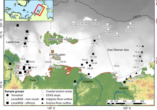
Figure 1. Map of the East Siberian Arctic Shelf (ESAS) showing the location of surface sediment and permafrost samples used in this study. The thin black line represents the −100 m bathymetric contour. Grey to white colours offshore represent the transition from −100 to 0 m water depth, highlighting both the shallow nature of the ESAS and the minor bathymetric features present. Major rivers are labelled. Areas of rapid coastal erosion (> 1 m yr−1; Lantuit et al., 2011) are shown in red. Groups of samples are denoted by marker shape and colour: black circles is terrestrial ICD and permafrost cores, white triangles is nearshore Lena River outflow/Buor-Khaya Bay, black squares is offshore Lena River outflow/Buor-Khaya Bay, white squares is areas of high coastal erosion and little fluvial input, white circles is distal ESAS areas, black pentagons is Indigirka River outflow and black triangles is Kolyma River outflow.
optimum combination of peak location, width and height us-ing the best-fit algorithms implemented by the open-source software package Gnuplot (version 4.6). A linear background subtraction was made as part of this automated fitting. For full details of the fitting process, see Sparkes et al. (2013). The fitting script used in this study is included as a support-ing file and developed at https://github.com/robertsparkes/ raman-fitting (last access: 29 September 2018).
As well as peak shape parameters (location, height, width, area), the fitting script calculates two additional values. The implied maximum burial temperature experienced by the car-bonaceous material is calculated based on the peak area ratio. For mildly and highly graphitised material, fitted using three Voigt peaks, the R2 ratio compares the G, D1 and D2 peaks (Beyssac et al., 2002b):
R2 = D1
G + D1 + D2. (1)
For more disordered CM fitted using five Lorentzian peaks, the RA2 ratio compares the G, D1, D2, D3 and D4
Lorentzian peaks (Lahfid et al., 2010): RA2 = (D1 + D4)
(G + D2 + D3). (2)
The temperature value derived from these calculations rep-resents the degree of graphite crystallinity in the carbona-ceous material. Highly graphitic samples have higher meta-morphic temperatures, up to 650◦C (Beyssac et al., 2002a). Less graphitised samples have lower temperatures, calibrated down to 200◦C (Lahfid et al., 2010). It relates to the peak metamorphic conditions experienced by the CM (Beyssac et al., 2002b), and when dealing with sedimentary samples is used as a tracer for CM from different lithologies (Sparkes et al., 2013). The second parameter is the sum of peak widths parameter, which is the sum of the G, D1 and D2 peak widths at half-maximum. This value is lowest for highly graphi-tised CM and increases with increasing CM disorder. Al-though it is a non-standard method for classifying Raman spectra, this parameter differentiates CM better than other potential parameters. For example, measuring just the width
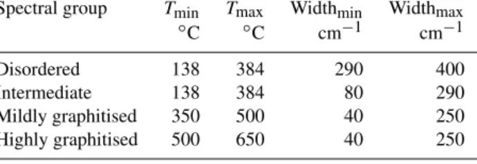
Table 1. Parameters for classifying Raman spectra into four groups based on their metamorphic temperature (determined from the R2 or RA2 peak area ratio; see Sparkes et al., 2013) and total width parameter (G + D1 + D2). Note that there are overlaps between the defined regions. Mildly graphitised takes precedence over interme-diate grade if a sample plots in the overlapping region.
Spectral group Tmin Tmax Widthmin Widthmax ◦ C ◦C cm−1 cm−1 Disordered 138 384 290 400 Intermediate 138 384 80 290 Mildly graphitised 350 500 40 250 Highly graphitised 500 650 40 250
of peak D1 can limit the ability to differentiate between mod-erately and extremely disordered CM, as the D1 peak width saturates at high amounts of disorder. When analysing only mildly and highly graphitised CM, the D1 width parameter could be used instead of total width. Extremely disordered CM has the highest total width value, and this factor can be used to discriminate between samples that are mildly meta-morphosed (and legitimately sit on the calibration of Lah-fid et al., 2010) and those that have undergone only dia-genetic alteration (e.g. lignite-grade CM). These extremely low-grade CM particles, for which metamorphic tempera-ture calibrations are not available, can still be distinguished and identified via their Raman spectra despite the lack of calibrated temperature (Sparkes et al., 2013). Using a com-bination of these two parameters, spectra were divided into four classes: disordered, intermediate, mildly graphitised and highly graphitised (see Table 1).
3 Results
3.1 Raman spectra collection
The 1463 spectra collected span the entire range from per-fectly crystalline graphite to highly disordered CM. Max-imum implied metamorphic temperatures were 641◦C, i.e. spectra with no discernible D1 peak. The highest total peak width values were 366 cm−1, i.e. extremely disordered spec-tra implying minimal CM crystallinity. Between these two endmembers, a complete range of spectra was collected. When rastering the microscope focus point across the ples, CM was easiest to find and measure in nearshore sam-ples. CM in samples collected from the distal shelf was more disperse and often consisted of smaller particles. However, since samples were ground before analysis, the size of each CM particle was not recorded.
3.2 Grouping spectra by Raman parameters
For each sample, Raman spectra were classified into disor-dered, intermediate, mildly graphitised and highly
graphi-tised CM as described above. This allowed the proportion of each spectral type in each sample to be investigated sta-tistically. The most common group of spectra was interme-diate, comprising 50 % of the data set, 27 % of the spec-tra were classified as disordered, 18 % as mildly graphitised and 5 % as highly graphitised. Based on the location of sam-ples on the shelf and guided by the proportion of spectra in each group, groupings were defined for various regions of the ESAS (Fig. 1) as follows:
1. Terrestrial samples. These comprised the Kurungnakh Island permafrost core, and permafrost samples col-lected from the Indigirka and Kolyma catchments. 2. Nearshore Buor-Khaya Bay. This group contained
sam-ples that were collected within 55 km of outflows from the Lena River (as measured by ArcGIS – see values in the Sample Metadata table in the Supplement).
3. Offshore Buor-Khaya Bay. These samples were col-lected further than 55 km from outflows of the Lena River.
4. Coastal erosion. This group comprised samples that were collected from areas known to have high rates of coastal erosion (Lantuit et al., 2011). This includes the Dmitry Laptev Strait, samples 31, 32 and YS-33, which lie to the west of the Kolyma River, and sam-ple YS-37, which lies near Ayon Island. According to Lantuit et al. (2011), Ayon Island is eroding slowly (0– 1 m yr−1) compared to the Dmitry Laptev Strait and re-gions west of Kolyma (2–10 m yr−1). However, sample
YS-37 was included in the coastal erosion group since the proximity of sample YS-37 to the island (20 km) is significantly lower than its proximity to the Kolyma River (245 km), and the spectral distribution in sample YS-37 is significantly different if compared to neigh-bouring samples in the Kolyma region (34 to YS-41; see Fig. 2).
5. Distal ESAS. This group contained the samples located furthest offshore, at the edge of the shelf and the start of the continental slope. The ESAS is particularly shallow for hundreds of kilometres offshore, and these samples were collected in water depths ranging from 32 to 69 m. 6. Indigirka outflow. This group comprised a transect of samples from the mouth of the Indigirka River onto the ESAS.
7. Kolyma outflow. This group comprised a transect of samples from the mouth of the Kokyma River onto the ESAS.
Within each of these sample groups, the distribution of spec-tra is shown in Fig. 3 and Table 2.
! ! ! ! ! ! ! ! ! ! ! ! ! ! ! ! ! ! ! ! !! ! ! !! ! ! ! ! ! ! ! ! ! ! ! ! ! ! ! ! ! ! ! ! ! ! ! ! 160° E 140° E 75 ° N 70 ° N 70 ° N 18 0° 12 0° E 0 50100 200 300 400 km Disordered Intermediate Mildly graphitised Highly graphitised
Figure 2. Raman spectroscopy results showing the relative amount of each carbonaceous material spectral class within each sample as pie charts.
3.3 Distribution of spectral classes within each group of samples
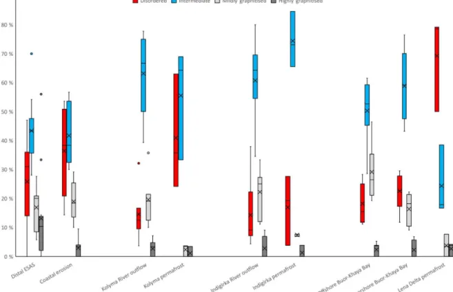
The terrestrial group contains the largest proportion of dis-ordered CM (42 %) and the smallest proportion of mildly graphitised (5 %) and highly graphitised CM (2 %). There is no apparent difference with depth in the terrestrial samples (KUR, KY, CH). The Buor-Khaya Bay nearshore and off-shore samples contain much less disordered CM than the ter-restrial Kurungnakh Island core samples (23 % and 18 % for the BKB vs. 68 % for the Kurungnakh Island core samples) and contain an increasing amount of mildly graphitised CM offshore (16 % and 29 %). Indigirka River and Kolyma River outflow samples contain the highest amounts of intermedi-ate CM (61 % and 63 % respectively) and the lowest propor-tion of disordered CM (14 % and 15 %). In contrast, coastal erosion samples contain relatively high proportions of disor-dered CM (36 %) and the joint-lowest amount of intermedi-ate CM (42 %). Distal ESAS samples contain 43 % interme-diate CM and the highest amount of highly graphitised CM (13 %). The highest amount of highly graphitised CM was found in the two samples positioned furthest from the con-tinental mainland, excluding the New Siberian Islands, (YS-104 (56 %) and YS-102 (33 %); see Fig. 2).
4 Discussion
4.1 Principal component analysis of spectral groups In order to observe patterns in the spectral classes between samples and sample groups, principal component analysis
(PCA) was applied using the software package R (R Core Team, 2015). For each sample, the proportion of each spec-tral class was analysed (e.g. Ndisordered/Ntotal), and principal
components were derived using the prcomp function. Due to the extreme amounts of highly graphitised CM in samples YS-102 and YS-104, the analyses were run with (see Sup-plement Fig. S3) and without (see Fig. 4) these two samples to investigate whether they biased the results. Considering that there was no significant difference between the two PCA analysis runs, except that the large amount of highly graphi-tised CM in samples YS-102 and YS-104 created a greater amount of scatter in the distal ESAS group, the PCA calcu-lations excluding samples YS-102 and YS-104 are used in further discussions.
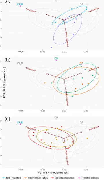
Principal component 1, explaining 74 % of the variance, shows the interplay between intermediate and disordered CM. These two spectral classes are plotted in opposition to each other. Principal component 2, explaining 22 % of the variance, denotes the relative enrichment in mildly graphi-tised CM. Principal component 3, representing only 4 % of the variance, contains the varying amount of highly graphi-tised CM, but is a minor component and the distribution of this material will be discussed in Sect. 4.3. The various sam-ple groups defined in Table 1 are plotted in well-defined re-gions (see Fig. 4).
The Kurungnakh Island core is plotted in the top left cor-ner of Fig. 4a. This position is noticeably different to the Buor-Khaya Bay samples, suggesting that bulk sediment de-livered from the Lena River is not the same as permafrost in the downstream area. Since the Lena catchment is one of the largest on Earth, this is not surprising. The nearshore BKB
Figure 3. Box and whisker chart showing the mean, median and quartile proportions of each spectral class within each group of samples. Sample groups are mapped in Fig. 1 and listed in the Sample Metadata table in the Supplement.
Table 2. Distribution of spectral classes within each group of samples. Percentage values are averages of the proportions within each group, rather than the proportion of the entire group. This corrects for samples in which it was not possible to collect 30 Raman spectra.
Sample group nsamples nspectra Disordered Intermediate Mildly Highly
graphitised graphitised
Lena Delta permafrost 3 80 69 % ± 14 % 24 % ± 10 % 4 % ± 3 % 3 % ± 2 %
BKB – nearshore 5 132 23 % ± 6 % 59 % ± 11 % 16 % ± 5 % 2 % ± 3 % BKB – offshore 7 197 18 % ± 6 % 50 % ± 10 % 29 % ± 9 % 2 % ± 2 % Indigirka permafrost 3 81 17 % ± 10 % 74 % ± 8 % 7 % ± 0 % 1 % ± 2 % Indigirka outflow 7 134 14 % ± 11 % 61 % ± 13 % 22 % ± 8 % 3 % ± 4 % Kolyma permafrost 3 84 41 % ± 16 % 56 % ± 16 % 2 % ± 2 % 1 % ± 2 % Kolyma outflow 7 188 15 % ± 8 % 63 % ± 13 % 20 % ± 8 % 3 % ± 3 % Coastal erosion 8 244 36 % ± 14 % 42 % ± 10 % 19 % ± 6 % 3 % ± 3 % Distal ESAS 13 325 26 % ± 14 % 43 % ± 10 % 17 % ± 7 % 13 % ± 15 %
samples are noticeably different to the offshore BKB ples, as shown by their confidence ellipses. Nearshore sam-ples have higher values of PC1 compared to the Kurungnakh Island core (average 0.06 ± 0.12 c.f. −0.5; all errors given as 1 standard deviation), but show a range of PC2 values ranging from nearly equivalent to substantially lower (aver-age 0.05 ± 0.06, range −0.03 to 0.13, c.f. 0.16). Offshore BKB samples have similar PC1 values to the nearshore sam-ples (average 0.04 ± 0.10), with a lower PC2 value (aver-age −0.11 ± 0.11). This denotes a high amount of disordered
CM and a low amount of intermediate and mildly graphi-tised CM in the Kurungnakh Island core compared to the BKB samples and that the offshore BKB samples contain more mildly graphitised CM than the nearshore BKB sam-ples. This could be a degradation or distribution effect, or it could be that the BKB offshore samples have less influence from the Lena outflow and more influence from coastal ero-sion within the Buor-Khaya Bay, such as Moustakh Island (Vonk et al., 2012).
● ● ● ● ● ● ● ● ● ● ● ● ● ● ● ● ● ● ● ● ● ● ● ● ● ● ● ● ● Disordered Intermediate Mildly grapitised −0.3 −0.2 −0.1 0.0 0.1 0.2 −0.50 −0.25 0.00 0.25 PC1 (73.7 % explained var.) ● ● ● ● ● ● ● ● ● ● ● ● ● ● ● ● ● ●● KUR CH KY ● ● ● ● ● ● ● ● ● ● ● ● ● ● ● ● ● ● ● ● ● ● Disordered Intermediate Mildly grapitised −0.3 −0.2 −0.1 0.0 0.1 0.2 −0.50 −0.25 0.00 0.25 P C 2 (2 2. 1 % e xp la in ed v ar .) ● ● ● ● ● ● ● ● ● ● ● ● ● ● ● ● ● ● ● ● ● ● ● ● ●● KUR CH KY ● ● ● ● ● ● ● ● ● ● ●● ● Disordered Intermediate Mildly grapitised −0.3 −0.2 −0.1 0.0 0.1 0.2 −0.50 −0.25 0.00 0.25 ● ● ● ● ● ● ● ● ● ● ● ● ● ● ● ● ● ● ● ● ● ● ● ● ● ● ● ● ● ● ● ● ● KUR ● CH ● KY ● ●
Coastal erosion areas ●
●
Indigirka River outflow Kolyma River outflow
● ● BKB - nearshore BKB - offshore ● Terrestrial samples (a) (b) (c) Distal ESAS
Figure 4. Principal component analysis plots of PC2 vs. PC1 for the sample groups. Terrestrial samples are shown individually. Vectors showing the contribution of spectral classes to the principal compo-nents are shown in red. Confidence ellipses (1 standard deviation) are shown in colours matching the sample groups. (a) Buor-Khaya Bay nearshore and offshore groups. (b) Kolyma and Indigirka river outflows. (c) Coastal erosion and distal ESAS groups. Data labels showing sample names are included in Supplement Fig. S2.
Onshore permafrost samples from the Indigirka and Kolyma catchments have high values of PC2 (0.171 and 0.218 respectively), which is similar to the Kurungnakh Is-land core and denotes a low amount of mildly graphitised CM. Offshore, the Indigirka and Kolyma outflows are plotted in similar locations on Fig. 4b. Their respective PC1 values are 0.14±0.16 and 0.15±0.14; PC2 values are −0.02±0.10 and 0.01 ± 0.10. These PC1 values are the highest of all sam-ple groups, denoting that the river outflows are the richest
in intermediate CM and poorest in disordered CM of the whole ESAS data set. As seen in the Bour-Khaya Bay, the offshore Indigirka and Kolyma samples have lower PC2 val-ues than the corresponding terrestrial samples, suggesting a higher amount of mildly graphitised CM offshore.
The coastal erosion data set has relatively low values of PC1 (average −0.15 ± 0.16) and PC2 values (−0.00 ± 0.08), which are similar to the Kolyma, Indigirka, distal ESAS and nearshore BKB groups. The low PC1 values denote a high amount of disordered CM in this group, which is supported by the trend within the sample set as a whole – the confi-dence ellipse in Fig. 4c for this group lies along the vector for disordered CM.
Samples from the distal ESAS have similar principal com-ponent values to the coastal erosion samples. PC1 averages −0.08 ± 0.15; PC2 0.00 ± 0.07. This set of values denotes that, similar to the coastal erosion group, the distal ESAS sediments contain high proportions of disordered CM, low proportions of intermediate CM and moderate amounts of mildly graphitised CM (more than the terrestrial samples, but less than the offshore Buor-Khaya Bay). It is noticeable that the distal ESAS confidence ellipse in Fig. 4c almost overlays the coastal erosion ellipse and is different to the ellipses from river outflow groups (Buor-Khaya Bay, Indigirka, Kolyma). This suggests that the distal ESAS sediments are mostly sourced from coastal erosion and that on-shelf homogenisa-tion processes are not sufficient to mix coastal-erosion- and river-derived sediments (see sedimentological data from Tesi et al., 2016).
4.2 Spatial pattern of principal component 1
To investigate further, the value principal component 1 was plotted across the ESAS (Fig. 5; Supplement Fig. S4). It shows that the Dmitry Laptev Strait, the region between the Indigirka and Kolyma rivers, and the north-eastern part of the distal ESAS have the lowest values of PC1. Highest values of PC1 are in the outflows of the Indigirka and Kolyma rivers, and in the central distal part of the ESAS (around 150◦E).
In the offshore area of the Lena River, the variation is more moderate, trending from mildly positive (somewhat enriched in intermediate OC) near the river to mildly negative (some-what enriched in disordered OC) on the ESAS at 130◦E. These patterns demonstrate that there are longitudinal zones of disordered and intermediate CM across the entire ESAS. In the western section, disordered CM is prevalent offshore in contrast to the Buor-Khaya Bay sediments. The permafrost core from Kurungnakh Island is enriched in disordered CM, as are the samples from the Dmitry Laptev Strait, which is known to have high rates of coastal erosion. This sug-gests that distal sediment in this region may be dominated by coastal erosion of permafrost, and that sediment from the Lena River is less likely to be deposited in the area north of the Lena Delta.
160° E 140° E 75 ° N 70 ° N 70 ° N 18 0° 0 50 100 200 300 400 km Principal component 1 -0.35 (disorder dominated) 0.33 (intermediate dominated)
Figure 5. Spatial distribution of principal component 1 across the ESAS. An interpolated map of the distribution is included as Supplement Fig. S4.
In the central section, from 140 to 160◦E, PC1 has a pos-itive value on the distal ESAS; the proportion of disordered CM is low, while intermediate CM dominates. This distribu-tion is similar to that of the Indigirka River outflow at 150◦E. It is likely that the sediments from the Indigirka have been transported out to this part of the shelf. However, there is a possibility that the New Siberian Islands, which are much closer to the distal ESAS than the Indigirka Outflow, could be the source of this intermediate CM. Unfortunately there are no samples from the New Siberian Islands for comparison.
In the eastern part of the distal ESAS, beyond 160◦E, PC1 has a negative value that is similar to samples collected to the west of the Kolyma River outflow, but different to the sam-ples collected east of the outflow. Pyrolysis-GC-MS studies of macromolecular OC in this region suggest that most of the OC delivered by the Kolyma River is distributed to the east of the outflow and that the samples to the west of the out-flow are likely dominated by coastal erosion (Sparkes et al., 2016). This would imply that the distal ESAS sediments east of 160◦E are mostly composed of material eroded from the coastline between the Indigirka and Kolyma rivers, known to have high rates of coastal erosion (Lantuit et al., 2011). Material delivered by the Kolyma River may be travelling even further to the east, and future sample campaigns beyond 170◦E may find material that is more enriched in intermedi-ate CM.
4.3 Distribution of highly graphitised CM
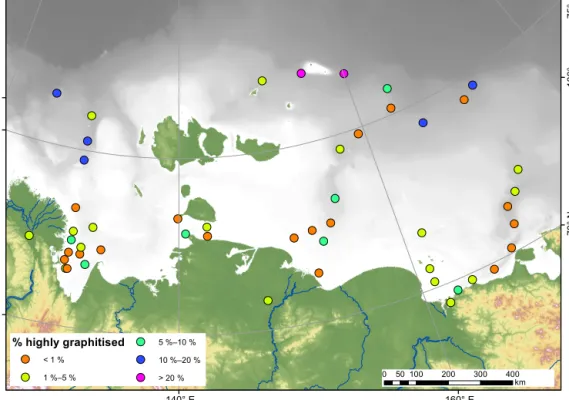
The relative proportion of highly graphitised CM in the dis-tal ESAS sample group was much higher than the other sam-ples (see Table 2 and Fig. 3). Throughout the distal ESAS group, highly graphitised CM represents 12 % of all spectra collected (38 spectra out of 325). Averaging the proportion of highly graphitised CM in each of these samples, the dis-tal ESAS group has 13 % ± 15 % (1 s.d.) highly graphitised CM, with a range from 0 % to 55 %. This heterogeneity is seen in Fig. 2, but there is still significantly (P = 0.0001) more highly graphitised CM in the distal ESAS group than the remaining samples (3 % ± 3 %), and the greatest propor-tion of highly graphitised CM found in any other sample is 10 % (sample YS-22). As mentioned earlier, two samples, YS-102 and YS-104, have extremely high amounts of highly graphitised CM, far exceeding the proportion measured in any other sample (33 % and 56 % respectively). Even with-out these samples in the calculation, the distal ESAS group is still significantly different from the remaining samples (7.4 % ± 5.5 % c.f. 3 % ± 3 %, P = 0.0001).
There is more highly graphitised CM in the distal ESAS samples than in both the nearshore ESAS samples and the terrestrial samples (1.7 % ± 1.9 % for terrestrial samples c.f. 7.4 % ± 5.5 % in the distal ESAS; P < 0.05). There is an in-creased amount of highly graphitised CM in the nearshore ESAS than the terrestrial samples, but this increase is not significant (2.7 % ± 2.9 % for the non-slope offshore
sam-! ! ! ! ! ! ! ! ! ! ! ! ! ! ! ! ! ! ! ! !! ! ! !! ! ! ! ! ! ! ! ! ! ! ! ! ! ! ! ! ! ! ! ! ! ! ! ! 160° E 140° E 75 ° N 75 ° N 70 ° N 70 ° N 18 0° 12 0° E 0 50100 200 300 400 km % highly graphitised < 1 % 1 %–5 % 5 %–10 % 10 %–20 % > 20 %
Figure 6. The distribution of highly graphitised CM across the ESAS. An interpolated map is included as Supplement Fig. S5.
ples, 1.7 % ± 1.9 % for terrestrial samples; P = 0.19). There-fore, there must be a process leading to an enhanced amount of highly graphitised CM present in the furthest offshore samples. Three possibilities exist for this: unseen sources of graphite, preferential preservation of graphite and sorting of sediment particles.
The terrestrial samples available for this project may not represent all of the eroded material from the ESAS. East-ern Siberia contains some of the world’s largest drainage basins and longest rivers, and therefore CM could be eroded from thousands of kilometres inland before being delivered to the ESAS. Highly graphitised CM has been shown to sur-vive long-distance river transport (Bouchez et al., 2010; Galy et al., 2007). There could be a source of graphite inland that, coupled with sorting effects, is responsible for the offshore graphite. In this case, rivers would deliver highly graphitised CM that is diluted by erosion of non-graphitic CM close to the river mouth and along the coastline. Further processing offshore, either the loss of non-graphitic CM or the concen-tration of graphitic CM, means that, while the graphite is a minor component of the nearshore samples, it can be seen in the distal samples.
However, samples collected near to the Lena and Indi-girka river mouths show no increase in graphite compared to nearby areas dominated by coastal erosion, suggesting that there is not even a diluted graphite signature coming from the rivers. Nearshore BKB samples (2.3 % ± 2.9 %) and the sam-ple nearest to the Indigirka River (YS-30; 0 %) have little or
no highly graphitised CM. The sample closest to the Kolyma River outflow has some highly graphitised CM (YS-34; 7 %), so there may be graphite erosion from within the Kolyma catchment. Nokleberg et al. (1993) report graphite bearing ore bodies from multiple locations within the Kolyma catch-ment, which form part of the Kolyma–Omolon superter-rane metamorphic belt. This material could survive trans-port through the Kolyma River (Bouchez et al., 2010), ex-plaining the increase in highly graphitised CM in the north-eastern part of the ESAS. Given the increasing proportion of highly graphitised CM observed offshore across the entire E–W transect, it is more likely that the graphite is sourced in low concentrations across the region and that offshore pro-cesses are responsible for increasing the proportion in distal areas.
Regardless of the graphite source, other processes are re-quired to explain the offshore trend in highly graphitised CM. There is a clear offshore transition from lower to greater amounts of highly graphitised CM (Fig. 6; Supple-ment Fig. S5), which could have been caused by a preserva-tion effect. As seen in transects along the Bengal Fan, there is often a trend to more crystalline graphite with transport distance (Galy et al., 2007). This has been explained as a re-sistance to physical, chemical and/or biological degradation. If disordered, intermediate or mildly graphitised CM is pref-erentially degraded during transport across the ESAS, distal samples would be relatively enriched in highly graphitised CM even if the proportion of this material in the sediment
delivered to the shelf is low, but there is not an offshore trend in the other classes of spectra. If graphitisation increases re-silience to degradation, it would be expected that disordered CM was the least resistant group of CM, and that this would be seen as a trend away from disordered CM offshore. How-ever, this is not the case and the distal ESAS samples contain large amounts of disordered CM. All CM analysed in this study must be autochthonous, even disordered CM. In situ production or flocculation of marine organic matter could not produce Raman-amenable CM particles.
There could also be a sorting effect across the shelf, rather than degradation. Whereas solvent extractable biomarkers of terrestrial processes have been shown to reduce rapidly across the ESAS (Bröder et al., 2016; Bischoff et al., 2016; Sparkes et al., 2015), most of the Raman-amenable CM present in these samples is likely to be resistant to degra-dation (Galy et al., 2008). Therefore, an alternative reason for highly graphitised CM to be present in high concentra-tions on the distal ESAS is that it is preferentially delivered and deposited there. Tesi et al. (2016) showed that organic carbon was mostly associated with fine particles in the dis-tal ESAS, and that larger particulate OC was deposited close to the coastline. Graphite flakes have a lower density than many silicate minerals and have a tabulate form. Winnow-ing is used commercially to separate graphite flakes from bulk sediments using liquid froth or air jet (Mitchell, 1993). Stokes’ law predicts that low-density graphite flakes travel-ling independently should settle slower than denser silicate minerals or large conglomerate grains. Less graphitic CM may be part of a sedimentary conglomerate or the individ-ual particles may be larger and have a higher settling veloc-ity. Thus, even if highly graphitised CM is present as only a minor fraction in the bulk sedimentary input to the ESAS, if other fractions are preferentially deposited on the shelf, then the most distal samples will be enriched in highly graphitised CM.
The current data set does not allow a definitive determi-nation of whether degradation or distribution is the primary cause of the offshore trend towards highly graphitised CM. The distal ESAS samples are located in deeper water com-pared to the other sample groups (see the Sample Metadata table in the Supplement). The deeper water setting allows increased settling time before burial, which would enhance both degradation and winnowing effects. It is noticeable, however, that there are no offshore trends in the distribution of disordered, intermediate or mildly graphitised CM. There-fore, whichever process is driving the highly graphitised CM pattern must be mostly affecting only the crystalline parti-cles.
4.4 Comparison with soot black carbon
Soot black carbon (SBC) is a complementary portion of the recalcitrant OC load in the ESAS. Salvadó et al. (2017) stud-ied SBC using chemical methods (chemothermal oxidation
to remove non-SBC, followed by elemental analysis and sta-ble/radiocarbon isotope mass spectrometry), which allowed for quantification of SBC and source apportionment. This method does not directly measure the nature of SBC parti-cles, in contrast to Raman analysis, but allows for quantifica-tion rather than investigating relative changes. They showed that, while the total amount of SBC diminished offshore, along with the proportion of SBC as a fraction of total OC, the proportion of SBC as a fraction of permafrost-sourced OC increased offshore, especially in the eastern ESAS. This pattern matches our findings regarding the proportion of highly graphitised CM in the ESAS sediments (see Figs. 3 and 4). The authors concluded that SBC is recalcitrant com-pared to other forms of permafrost OC and avoids degrada-tion during transport. Our Raman study supports this finding, while also adding information about the longitudinal distri-bution of CM. Longitudinal variations in SBC amount, pro-portion and radiocarbon signature are small, but Raman sug-gests that river-sourced and coastal-erosion-sourced recalci-trant organic matter can be differentiated and tracked across the shelf.
One consideration when comparing the chemical SBC and spectroscopic Raman studies is whether there is crossover between the two carbon pools. SBC particles can have a wide range of chemical structures and grain sizes. Some SBC grains may be large enough to be seen using a Raman micro-scope (greater than approx. 5 µm), but most SBC particles are smaller than submicron size and would not be analysed. Some CM, especially highly graphitised CM, may survive the chemothermal oxidation process and be counted amongst the SBC pool. Intermediate and disordered grade CM are more likely to be lost during the chemothermal oxidation, and it is these two forms of CM that demonstrated longitu-dinal variation, highlighting the difference between river and coastal permafrost carbon. Thus, there is value in measur-ing both the chemical properties and crystallographic form of recalcitrant organic matter as a way of tracking exported carbon and sediment.
4.5 Implications for carbon cycling in the ESAS The results of this study indicate that terrestrially sourced CM in the East Siberian Arctic region can be found in sed-iments hundreds of kilometres offshore. Whilst direct quan-tification of CM as a fraction of total OC is not possible us-ing Raman spectroscopy, chemical analyses show that SBC could account for 14 % of terrestrial OC in distal sediments (Salvadó et al., 2017). Highly graphitised CM is structurally similar to SBC and the chemothermal treatment used in these studies likely removes low-grade CM, implying that CM concentrations could be similar to, if not higher than, SBC offshore.
Whereas biomarker studies suggest that terrestrially sourced organic compounds are often absent or have very low concentrations in offshore settings in this region (Sparkes
et al., 2015; Bischoff et al., 2016; Do˘grul Selver et al., 2015; Bröder et al., 2016), CM was observed in every offshore sample and there does not seem to be a consistent decline in any of the CM groups – there are distal ESAS samples with significant proportions of each of these classes. Halfway between extractable lipids and Raman-amenable CM parti-cles is macromolecular organic matter, such as lignin. Tesi et al. (2014) extracted these same samples and found that concentrations of lignin phenols were also very low in the outer shelf. Thus, the CM observed using Raman behaves very differently to extractable and pyrolysable OC. While there are observable offshore trends, it appears that this ma-terial is much more resilient than the labile organic matter traditionally used to track OC export from terrestrial settings. This observation likely accounts for the old radiocarbon val-ues observed in ESAS sediments (Sparkes et al., 2016; Vonk et al., 2012), where carbon eroded from coastal sediments is thought to be a major contributor to offshore sedimentary OC, whereas modern terrestrial OC is a minor component far offshore. CM has undergone diagenesis and/or metamor-phism, a process that takes a significant amount of time and should therefore have no radiocarbon remaining. Conserva-tive offshore transport also addresses the anomalous radio-carbon values measured in the Beaufort Sea by Goñi et al. (2005). If CM can be transported for large distances offshore without significant degradation, it could lead to unusually old radiocarbon in seafloor sediments but potentially also sus-pended particulate matter.
Long-distance CM transport also has implications for the carbon cycle in this region. Vonk et al. (2012) esti-mated, using bulk isotope analysis, that 66 % ± 16 % of the 44 ± 10 Tg OC eroded from ice complexes along the ESAS coastline is released as CO2, with the remaining third buried
in the shelf or deep ocean. Distal shelf sediments were esti-mated as containing up to 50 % of their OC from coastal ero-sion sources. However, subsequent molecular analyses have suggested that organic matter degradation is extremely preva-lent by the outer shelf. Solvent extractable material, while only accounting for 5 % to 10 % of the total OC content of exported sediment, have predicted a significant loss of terres-trial OC during transport across the ESAS (Bischoff et al., 2016; Bröder et al., 2016; Karlsson et al., 2015; Sparkes et al., 2015; Tesi et al., 2014). Pyrolysis GC-MS, investi-gating larger, non-extracted, biomolecules, also found that terrestrial markers were much diminished on the outer shelf (Sparkes et al., 2016). Therefore, this study provides a sys-tematic characterisation of the most likely form of terres-trial carbon in distal offshore settings. Erosion of recalcitrant OC from permafrost, without subsequent degradation, will transpose carbon from land into ESAS sediments or the deep Arctic Ocean basin, with no net effect on atmospheric CO2
levels. If the recalcitrant CM analysed in this study forms a significant proportion of the OC load of the ESAS, then the warming-induced carbon cycle feedbacks will not be as se-vere as if all terrestrial OC was degraded. Thus, when
mod-elling the impact of permafrost erosion on climate change, and vice versa, researchers should not consider the total or-ganic carbon content of the mobilised sediment but its labile fraction. Note that some of this labile fraction could be an-cient carbon, currently locked in permafrost deposits across Eastern Siberia (Tarnocai et al., 2009), and therefore per-mafrost thaw can still cause a net increase in atmospheric CO2levels and an associated positive feedback relationship
with climate warming.
5 Conclusions
Raman spectroscopy of carbonaceous material has been suc-cessfully applied across the East Siberian Arctic Shelf, a complex and heterogeneous sedimentary system. By group-ing collected spectra into classes and applygroup-ing principal com-ponent analysis, CM from river and coastal erosion has been differentiated – coastal erosion delivers more disordered CM, while rivers deliver more intermediate CM. Across the ESAS, two main processes have been identified. Firstly, there is a trend across the entire shelf towards highly graphi-tised CM in the furthest offshore samples, collected from the distal ESAS. This could be due to degradation of weaker CM during transport or preferential winnowing of crystalline graphite to more distal settings; given the presence of disor-dered CM in the most distal settings, winnowing is the pre-ferred explanation. In addition to this, an east–west pattern is observed in the distribution of disordered and intermediate CM. This suggests that there are areas where sedimentation is dominated by material sourced from rivers and areas domi-nated by coastal erosion sediment. Despite the shelf being ex-tremely wide and shallow, sediment transport processes have not homogenised the sediments and three individual sections can be identified along the shelf. Raman spectroscopy is thus a valuable tool for identifying and tracking eroded sediment in complex environments. Furthermore, the presence of CM ranging from disordered to highly graphitised in distal sedi-ments, hundreds of kilometres from the coastline, shows that Raman-amenable carbon is generally resistant to oxidation and thus a conservative part of the organic carbon cycle in this region.
Code and data availability. Supplementary information is supplied with this paper.
Supplementary information included with the article:
– Sample Metadata: a spreadsheet containing sample locations, previously measured geochemical parameters and results from principal component analysis.
– Supplementary Figure S1: an example of peak-fitting results for disordered/intermediate, mildly graphitised and highly graphitised spectra.
– Supplementary Figure S2: principal component analysis re-sults, as shown in Fig. 4, but with each sample location identi-fied.
– Supplementary Figure S3: principal component analysis re-sults if samples YS-102 and YS-104 are also included in the procedure.
– Supplementary Figure S4: interpolated map of principal com-ponent 1 across the ESAS. Interpolation was carried out using the nearest-neighbour algorithm within ArcMap.
– Supplementary Figure S5: interpolated map of percentage highly graphitised CM across the ESAS. Interpolation was car-ried out using the nearest-neighbour algorithm within ArcMap. Colour scale transition has a geometric profile to enable re-gions with smaller amounts of highly graphitised CM to be differentiated.
Supporting data and code underlying this study are available via the MMU research repository:
– The shell script used to fit Raman data: https://doi.org/10. 23634/MMUDR.00620208 (Sparkes, 2018)
– Unprocessed Raman spectra as x,y text files: https://doi.org/10. 23634/MMUDR.00620205 (Sparkes et al., 2018)
– Fitted spectra, showing the automatically fitted peaks, as a PDF file: https://doi.org/10.23634/MMUDR.00620207 (Sparkes and Maher, 2018a)
– Parameters of the fitted peaks including height, width, lo-cation and area: https://doi.org/10.23634/MMUDR.00620209 (Sparkes and Maher, 2018b)
Raman fitting procedures are also published and main-tained at https://github.com/robertsparkes/raman-fitting (last ac-cess: 29 September 2018).
Supplement. The supplement related to this article is available online at: https://doi.org/10.5194/tc-12-3293-2018-supplement.
Author contributions. ÖG, BEvD, and IPS collected samples along with the crew of ISSS-08. RBS designed the study. ADS assisted in preparing the samples for analysis. Raman spectroscopy measure-ments were carried out by MM, JB and RBS. Data analysis was carried out by RBS. RBS and BEvD prepared the manuscript with contributions from all co-authors.
Competing interests. The authors declare that they have no conflict of interest.
Acknowledgements. We gratefully acknowledge receipt of NERC research grants (NE/I024798/1 and NE/P006221/1) to Bart E. van Dongen, an MMU studentship to Robert B. Sparkes/Melissa Maher, an MMU-EERC research grant to Robert B. Sparkes, Swedish Research Council (VR contracts 621-2007-4631, 621-2013-5297 and the Distinguished Professors Grant 2017-01601) and the European Research Council (ERC-AdG CC-TOP project #695331) support to Örjan Gustafsson, and support from the Government
of the Russian Federation (mega-grant 14.Z50.31.0012) to Igor P. Semiletov. We thank the crew and personnel of the R/V Yakob Smirnitskyi and all colleagues in the International Siberian Shelf Study (ISSS) Program for support, including sampling. We thank Tomasso Tesi for providing the Yedoma samples for the Kolyma and Indigirka catchment areas. We thank Juliane Bischoff and Dirk Wagner for providing the Kurungnakh Island core. Hayley Andrews provided technical support for the MMU Raman Spectrometer. The ISSS program is supported by the Knut and Alice Wallenberg Foundation, the Far Eastern Branch of the Russian Academy of Sciences, the Swedish Research Council (VR contract no. 621-2004-4039, 621-2007-4631 and 621-2013-5297), the US National Oceanic and Atmospheric Administration (OAR Climate Program Office, NA08OAR4600758/Siberian Shelf Study), the Russian Foundation of Basic Research (08-05-13572, 08-05-00191-a, and 07-05-00050a), the Swedish Polar Research Secretariat, the Nordic Council of Ministers and the US National Science Foundation (OPP ARC 0909546). Finally, we thank the editor and two anonymous reviewers for their comments and suggestions.
Edited by: Florent Dominé
Reviewed by: two anonymous referees
References
Beyssac, O., Goffe, B., Chopin, C., and Rouzaud, J.: Ra-man spectra of carbonaceous material in metasediments: a new geothermometer, J. Metamorph. Geol., 20, 859–871, https://doi.org/10.1046/j.1525-1314.2002.00408.x, 2002a. Beyssac, O., Rouzaud, J., Goffe, B., Brunet, F., and Chopin, C.:
Graphitization in a high-pressure, low-temperature metamorphic gradient: a Raman microspectroscopy and HRTEM study, Con-trib. Mineral. Petr., 143, 19–31, https://doi.org/10.1007/s00410-001-0324-7, 2002b.
Beyssac, O., Brunet, F., Petitet, J.-P., Bruno Goffe, B., and Rouzaud, J.-N.: Experimental study of the microtextural and structural transformations of carbonaceous materials under pressure and temperature, Eur. J. Mineral., 15, 937–951, 2003a.
Beyssac, O., Goffe, B., Petitet, J.-P., Froigneux, E., Moreau, M., and Rouzaud, J.-N.: On the characterization of disordered and heterogeneous carbonaceous materials by Raman spectroscopy, Spectrochim. Acta, 59, 2267–2276, 2003b.
Beyssac, O., Simoes, M., Avouac, J., Farley, K., Chen, Y.-G., Chan, Y.-C., and Goffe, B.: Late Cenozoic metamorphic evolu-tion and exhumaevolu-tion of Taiwan, Tectonics, 26, TC6001–1–32, https://doi.org/10.1029/2006TC002064, 2007.
Bischoff, J., Mangelsdorf, K., Gattinger, A., Schloter, M., Kur-chatova, A. N., Herzschuh, U., and Wagner, D.: Response of methanogenic archaea to Late Pleistocene and Holocene climate changes in the Siberian Arctic, Global Biogeochem. Cy., 27, 305–317, https://doi.org/10.1029/2011GB004238, 2013. Bischoff, J., Sparkes, R. B., Do˘grul Selver, A., Spencer, R. G.
M., Gustafsson, Ö., Semiletov, I. P., Dudarev, O. V., Wag-ner, D., Rivkina, E., van Dongen, B. E., and Talbot, H. M.: Source, transport and fate of soil organic matter inferred from microbial biomarker lipids on the East Siberian Arctic Shelf, Biogeosciences, 13, 4899–4914, https://doi.org/10.5194/bg-13-4899-2016, 2016.
Bouchez, J., Beyssac, O., Galy, V., Gaillardet, J., France-Lanord, C., Maurice, L., and Moreira-Turcq, P.: Oxida-tion of petrogenic organic carbon in the Amazon floodplain as a source of atmospheric CO(2), Geology, 38, 255–258, https://doi.org/10.1130/G30608.1, 2010.
Bröder, L., Tesi, T., Salvadó, J. A., Semiletov, I. P., Dudarev, O. V., and Gustafsson, Ö.: Fate of terrigenous organic matter across the Laptev Sea from the mouth of the Lena River to the deep sea of the Arctic interior, Biogeosciences, 13, 5003–5019, https://doi.org/10.5194/bg-13-5003-2016, 2016.
Coppola, A. I., Ziolkowski, L. A., Masiello, C. A., and Druf-fel, E. R. M.: Aged black carbon in marine sediments and sinking particles, Geophys. Res. Lett., 41, 2427–2433, https://doi.org/10.1002/2013GL059068, 2014.
Do˘grul Selver, A., Sparkes, R. B., Bischoff, J., Talbot, H. M., Gustafsson, Ö., Semiletov, I. P., Dudarev, O. V., Boult, S., and van Dongen, B. E.: Distributions of bacterial and ar-chaeal membrane lipids in surface sediments reflect differ-ences in input and loss of terrestrial organic carbon along a cross-shelf Arctic transect, Org. Geochem., 83, 16–26, https://doi.org/10.1016/j.orggeochem.2015.01.005, 2015. Durand, B.: Kerogen: Insoluble Organic Matter from Sedimentary
Rocks, Editions technip, 1980.
Elmquist, M., Cornelissen, G., Kukulska, Z., and Gustafs-son, O.: Distinct oxidative stabilities of char versus soot black carbon: Implications for quantification and environ-mental recalcitrance, Global Biogeochem. Cy., 20, gB2009, https://doi.org/10.1029/2005GB002629, 2006.
Feng, X., Vonk, J. E., van Dongen, B. E., Gustafsson, Ö., Semile-tov, I. P., Dudarev, O. V., Wang, Z., Montluçon, D. B., Wacker, L., and Eglinton, T. I.: Differential mobilization of terrestrial carbon pools in Eurasian Arctic river basins, P. Natl. Acad. Sci. USA, 110, 14168–14173, https://doi.org/10.1073/pnas.1307031110, 2013.
Feng, X., Gustafsson, Ö., Holmes, R. M., Vonk, J. E., van Don-gen, B. E., Semiletov, I. P., Dudarev, O. V., Yunker, M. B., Macdonald, R. W., Wacker, L., Montluçon, D. B., and Eglinton, T. I.: Multimolecular tracers of terrestrial carbon transfer across the pan-Arctic: 14C characteristics of sedimentary carbon com-ponents and their environmental controls, Global Biogeochem. Cy., 29, 1855–1873, https://doi.org/10.1002/2015GB005204, 2015GB005204, 2015.
Ferrari, A. C.: Raman spectroscopy of graphene and graphite: Disorder, electron-phonon coupling, doping and nona-diabatic effects, Solid State Commun., 143, 47–57, https://doi.org/10.1016/j.ssc.2007.03.052, 2007.
Galy, V., France-Lanord, C., Beyssac, O., Faure, P., Kudrass, H., and Palhol, F.: Efficient organic carbon burial in the Bengal fan sustained by the Himalayan erosional system, Nature, 450, 407– 410, https://doi.org/10.1038/nature06273, 2007.
Galy, V., Beyssac, O., France-Lanord, C., and Eglinton, T.: Re-cycling of Graphite During Himalayan Erosion: A Geological Stabilization of Carbon in the Crust, Science, 322, 943–945, https://doi.org/10.1126/science.1161408, 2008.
Goñi, M. A., Yunker, M. B., Macdonald, R. W., and Eglin-ton, T. I.: The supply and preservation of ancient and mod-ern components of organic carbon in the Canadian Beau-fort Shelf of the Arctic Ocean, Mar. Chem., 93, 53–73, https://doi.org/10.1016/j.marchem.2004.08.001, 2005.
Gordeev, V. V.: Fluvial sediment flux to the
Arctic Ocean, Geomorphology, 80, 94–104,
https://doi.org/10.1016/j.geomorph.2005.09.008, 2006. Grigoriev, M. N., Rachold, V., and Bolshiyanov, D.:
ussian-German cooperation SYSTEM LAPTEV SEA: the expedition LENA 2002, Berichte zur Polar- und Meeresforschung (Re-ports on Polar and Marine Research), Bremerhaven, Alfred We-gener Institute for Polar and Marine Research, 466, 341 pp., https://doi.org/10.2312/BzPM_0466_2003, 2003.
Gustafsson, O., Bucheli, T. D., Kukulska, Z., Andersson, M., Largeau, C., Rouzaud, J.-N., Reddy, C. M., and Eglinton, T. I.: Evaluation of a protocol for the quantification of black carbon in sediments, Global Biogeochem. Cy., 15, 881–890, https://doi.org/10.1029/2000GB001380, 2001.
Gustafsson, Ö., van Dongen, B. E., Vonk, J. E., Dudarev, O. V., and Semiletov, I. P.: Widespread release of old carbon across the Siberian Arctic echoed by its large rivers, Biogeosciences, 8, 1737–1743, https://doi.org/10.5194/bg-8-1737-2011, 2011. Hilton, R. G.: Erosion of Organic Carbon from Active Mountain
Belts, PhD thesis, University of Cambridge, 2008.
Holmes, R. M., McClelland, J. W., Peterson, B. J., Shiklomanov, I. A., Shiklomanov, A. I., Zhulidov, A. V., Gordeev, V. V., and Bobrovitskaya, N. N.: A circumpolar perspective on fluvial sedi-ment flux to the Arctic ocean, Global Biogeochem. Cy., 16, 1098, https://doi.org/10.1029/2001GB001849, 2002.
Holmes, R. M., Coe, M. T., Fiske, G. J., Gurtovaya, T., McClelland, J. W., Shiklomanov, A. I., Spencer, R. G. M., Tank, S. E., and Zhulidov, A. V.: Climate Change Impacts on the Hydrology and Biogeochemistry of Arctic Rivers, John Wiley & Sons, Ltd, 1– 26, https://doi.org/10.1002/9781118470596.ch1, 2012.
IPCC: Climate Change 2013: The Physical Science Basis. Contri-bution of Working Group I to the Fifth Assessment Report of the Intergovernmental Panel on Climate Change, Tech. rep., 2013. Karlsson, E., Brüchert, V., Tesi, T., Charkin, A., Dudarev,
O., Semiletov, I., and Gustafsson, Ö.: Contrasting regimes for organic matter degradation in the East Siberian Sea and the Laptev Sea assessed through microbial incuba-tions and molecular markers, Mar. Chem., 170, 11–22, https://doi.org/10.1016/j.marchem.2014.12.005, 2015.
Kienast, F., Schirrmeister, L., Siegert, C., and Tarasov, P.: Palaeob-otanical evidence for warm summers in the East Siberian Arc-tic during the last cold stage, Quaternary Res., 63, 283–300, https://doi.org/10.1016/j.yqres.2005.01.003, 2005.
Kotlyakov, V. and Khromova, T.: Maps of Permafrost and Ground Ice, Version 1, in: Land Resources of Russia, 2002.
Kuznetsov, P., Kolesnikova, S., Kuznetsova, L., Okhlopkov, S., and Safronov, A.: Composition of Coals from Northern Fields of the Lena Coal Basin Estimating the Conversion into Liquid Fuel, Chemistry for Sustainable Development, 17, 35–41, 2009. Lahfid, A., Beyssac, O., Deville, E., Negro, F., Chopin,
C., and Goffe, B.: Evolution of the Raman spectrum of carbonaceous material in low-grade metasediments of the Glarus Alps (Switzerland), Terra Nova, 22, 354–360, https://doi.org/10.1111/j.1365-3121.2010.00956.x, 2010. Lantuit, H., Overduin, P. P., Couture, N., Wetterich, S., Aré, F.,
Atkinson, D., Brown, J., Cherkashov, G., Drozdov, D., Forbes, D. L., Graves-Gaylord, A., Grigoriev, M., Hubberten, H.-W., Jordan, J., Jorgenson, T., Ødegård, R. S., Ogorodov, S., Pol-lard, W. H., Rachold, V., Sedenko, S., Solomon, S., Steenhuisen,