On the numerical analysis of infinite multi-dimensional Markov chains

(1)

ON THE NUMERICAL ANALYSIS OF

INFINITE MULTI-DIMENSIONAL MARKOV

CHAINS

a dissertation submitted to

the graduate school of engineering and science

of bilkent university

in partial fulfillment of the requirements for

the degree of

doctor of philosophy

in

computer engineering

By

Muhsin Can Orhan

July 2017

(2)

ON THE NUMERICAL ANALYSIS OF INFINITE MULTI-DIMENSIONAL MARKOV CHAINS

By Muhsin Can Orhan July 2017

We certify that we have read this dissertation and that in our opinion it is fully adequate, in scope and in quality, as a dissertation for the degree of Doctor of Philosophy.

Tu˘grul Dayar(Advisor)

Nail Akar

Murat Manguo˘glu

Selim Aksoy

Mehmet Halit Seyfullah O˘guzt¨uz¨un Approved for the Graduate School of Engineering and Science:

Ezhan Kara¸san

(3)

ABSTRACT

ON THE NUMERICAL ANALYSIS OF INFINITE

MULTI-DIMENSIONAL MARKOV CHAINS

Muhsin Can Orhan Ph.D. in Computer Engineering

Advisor: Tu˘grul Dayar July 2017

A system with multiple interacting subsystems that exhibits the Markov prop-erty can be represented as a multi-dimensional Markov chain (MC). Usually the reachable state space of this MC is a proper subset of its product state space, that is, Cartesian product of its subsystem state spaces. Compact storage of the infinitesimal generator matrix underlying such a MC and efficient implementa-tion of analysis methods using Kronecker operaimplementa-tions require the set of reachable states to be represented as a union of Cartesian products of subsets of subsystem state spaces.

We first show that the problem of partitioning the reachable state space of a three or higher dimensional system with a minimum number of partitions into Cartesian products of subsets of subsystem state spaces is NP-complete. Two algorithms, one merge based the other refinement based, that yield possibly non-optimal partitionings are presented. Results of experiments on a set of problems from the literature and those that are randomly generated indicate that, although it may be more time and memory consuming, the refinement based algorithm almost always computes partitionings with a smaller number of partitions than the merge based algorithm.

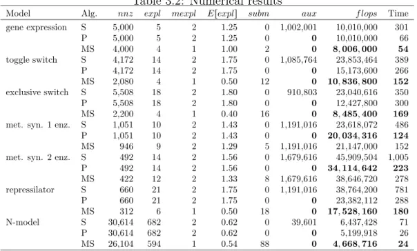
When the infinitesimal generator matrix underlying the MC is repre-sented compactly using Kronecker products, analysis methods based on vector– Kronecker product multiplication need to be employed. When the factors in the Kronecker product terms are relatively dense, vector–Kronecker product multipli-cation can be performed efficiently by the shuffle algorithm. When the factors are relatively sparse, it may be more efficient to obtain nonzero elements of the gener-ator matrix in Kronecker form on-the-fly and multiply them with corresponding elements of the vector. We propose a modification to the shuffle algorithm that multiplies relevant elements of the vector with submatrices of factors in which zero rows and columns are omitted. This approach avoids unnecessary floating-point

(4)

iv

operations that evaluate to zero during the course of the multiplication. Numer-ical experiments on a large number of models indicate that, in many cases the modified shuffle algorithm performs a smaller number of floating-point operations than the shuffle algorithm and the algorithm that generates nonzeros on-the-fly, sometimes with minimum number of floating-point operations and amount of memory possible.

Although the generator matrix is stored compactly using Kronecker products, solution vectors used in the analysis still require memory proportional to the size of the reachable state space. This becomes a bigger problem as the num-ber of dimensions increases. We show that it is possible to use the hierarchical Tucker decomposition (HTD) to store the solution vectors during Kronecker-based Markovian analysis relatively compactly and still carry out the basic oper-ation of vector–matrix multiplicoper-ation in Kronecker form relatively efficiently.

The time evolution of a stochastic chemical system modelled as a continuous-time MC (CTMC) can be described as a system of ordinary differential equations (ODEs) known as the chemical master equation (CME). The CME can be an-alyzed by discretizing time and solving a linear system obtained by truncating the countably infinite state space at each time step. However, it is not trivial to choose a truncated state space that includes few states with negligible probabili-ties and leaves out only a small probability mass. We show that it is possible to decrease the memory requirement of the ODE solver using HTD with adaptive truncation strategies and we propose a novel approach to truncate the countably infinite state space using prediction vectors. Numerical experiments indicate that adaptive truncation strategies improve time and memory efficiency significantly when fixed truncation strategies are inefficient.

Finally, we consider a multi-class multi-server retrial queueing system in which customers arrive according to a class-dependent Markovian arrival pro-cess (MAP). Service and retrial times follow class-dependent phase-type (PH) distributions with the further assumption that PH distributions of retrial times are acyclic. Here, we obtain a necessary and sufficient condition for ergodicity from criteria based on drifts. The countably infinite state space of the model is truncated with an appropriately chosen Lyapunov function. The truncated model is described as a multi-dimensional MC and a Kronecker representation of its infinitesimal generator matrix is numerically analyzed.

Keywords: Markov chain, Kronecker representation, Cartesian product partition-ing, vector–Kronecker product multiplication, hierarchical Tucker decomposition,

(5)

v

(6)

¨

OZET

SONSUZ C

¸ OK BOYUTLU MARKOV Z˙INC˙IRLER˙IN˙IN

SAYISAL C

¸ ¨

OZ ¨

UMLEMES˙I UZERINE

Muhsin Can Orhan

Bilgisayar M¨uhendisli˘gi, Doktora Tez Danı¸smanı: Tu˘grul Dayar

Temmuz 2017

Birden fazla alt sistemden olu¸san ve Markov özelli˘gine sahip bir sistemi ¸cok boyutlu bir Markov zinciri olarak göstermek mümkündür. Bu Markov zincirinin ula¸sılabilir durum uzayı, genellikle ¸carpım durum uzayının bir öz alt kümesidir. Böyle bir Markov zincirine kar¸sı gelen matrisin sıkı¸stırılmı¸s olarak saklanması ve Kronecker i¸slemlerin etkili bir ¸sekilde ger¸cekle¸stirilebilmesi, ula¸sılabilir durum uzayının alt sistem durum uzaylarının alt kümelerinin Kartezyen ¸carpımlarının birle¸simi olarak yazılmasını gerektirir.

Bu ¸calı¸smada ilk olarak, ü¸c veya daha fazla boyutlu bir sistemin ula¸sılabilir durum uzayının en az sayıda alt sistem durum uzaylarının alt kümelerinin Kartezyen ¸carpımlarına bölümleme probleminin, NP-tam bir problem oldu˘gunu gösteriyoruz. Bu problemi ¸cözmek i¸cin, eniyi ¸cözümü bulması kesin olmayan, biri birle¸stirme ve di˘geri geli¸stirme temelli olmak üzere iki algoritma öneriyoruz. Lit-eratürde yer alan ve rasgele olarak olu¸sturulmu¸s örneklerle yaptı˘gımız deneyler, geli¸stirme temelli algoritmanın daha ¸cok zaman ve bellek gerektirdi˘gini, ancak neredeyse her zaman daha az sayıda bölümleme bulabildi˘gini gösteriyor.

Markov zincirine kar¸sılık gelen matris, Kronecker ¸carpımları kullanılarak sıkı¸stırılmı¸s olarak gösterildi˘ginde, özümleme yöntemleri vektör–Kronecker terim ¸carpımının üzerine bina edilir. Kronecker terimlerdeki ¸carpan matrisler yo˘gun oldu˘gunda, karma algoritması vektör–Kronecker terim ¸carpımını etkili bir ¸sekilde hesaplayabilir. Ç arpan matrisler seyrek oldu˘gunda ise, Markov zincirine kar¸sılık gelen matrisin sıfırdan farklı elemanlarını ¸carpım esnasında olu¸sturup vektörde kar¸sılık gelen elemanlarla ¸carpmak daha etkili olabilmektedir. Karma algo-ritmasını, Kronecker terimin ¸carpan matrislerindeki tamamı sıfır olan satır ve sütünları gözardı edecek ¸sekilde de˘gi¸stirmeyi öneriyoruz. Bu de˘gi¸siklik, sonucu sıfır olan kayan noktalı sayı i¸slemlerinin ger¸cekle¸stirilmemesini sa˘glıyor. Ç ok sayıda modelde, de˘gi¸stirilmi¸s karma algoritması pek ¸cok kayan noktalı sayı

(7)

vii

i¸sleminden ka¸cınılmasını sa˘glıyor. Yine bazı modellerde, de˘gi¸stirilmi¸s karma al-goritmasının sıfırdan farklı elemenları ¸carpım esnasında olu¸sturan algoritmaya kıyasla daha az kayan noktalı sayı i¸slemi ve bellek gerektiriyor.

Markov zincirine kar¸sılık gelen matris, Kronecker ¸carpımları kullanılarak sıkı¸stırılmı¸s olarak gösterilse bile, i¸slemler i¸cin gereken bellek miktarı ula¸sılabilir durum uzayının büyüklü˘güyle do˘gru orantılı olarak de˘gi¸smektedir. Ozellikle¨ boyut sayısı arttı˘gında, bu daha büyük bir sorun olu¸sturmaktadır. Hiyerar¸sik Tucker ayrı¸stırması kullanarak, ¸cözüm vektörlerinin görece sıkı¸stırılmı¸s olarak tutulup, temel vektör–Kronecker terim ¸carpma i¸slemlerinin görece etkili olarak ger¸cekle¸stirilebildi˘gini gösteriyoruz.

Sürekli zamanlı bir Markov zinciri olarak modellenmi¸s bir rassal kimyasal sis-temin zamana ba˘glı de˘gi¸simi kimyasal ana denklemi olarak da bilinen bir adi diferansiyel denklem sistemi olarak tanımlanabilir. Kimyasal ana denklemi, za-manı ayrıkla¸stırarak ve saylabilir sonsuz durum uzayınının kesilerek elde edilmi¸s do˘grusal sistemin ¸cözülmesiyle ¸cözümlenebilir. Durum uzayının ihmal edilebilir az sayıda durum i¸cererek, kesilmi¸s durum uzayı dı¸sında az miktarda olasılık kitlesi kalacak ¸sekilde kesilmesi ise apa¸cık de˘gildir. Hiyerar¸sik Tucker ayrı¸stırması kul-lanarak adi diferansiyel denklem ¸cözücüsünün ihtiya¸c duydu˘gu bellek miktarını azaltılabilece˘gini gösteriyoruz. Ayrıca, sonsuz durum uzayını kesmek i¸cin tahmin vektörlerini kullanan yenilik¸ci bir yöntem öneriyoruz. Sayısal deneyler uyarlamalı kesim stratejilerinin zaman ve bellek ihtiyacını, sabit kesim stratejilerine kıyasla ciddi olarak azalttı˘gını gösteriyor.

Son olarak, birden fazla sınıfa ait mü¸steri kabul eden, mü¸sterilerin sınıfa ba˘gımlı Markov varı¸s sürecine göre geldikleri ve ¸cok sayıda sunucusu olan bir yeniden denemeli kuyruk sistemini ele alıyoruz. Ele aldı˘gımız sistemde, servis zamanlarınının sınıfa ba˘gımlı evre-tipli, yeniden deneme zamanlarının ise ¸cevrimsiz sınıfa ba˘gımlı evre-tipli da˘gılım gösterdiklerini farz ediyoruz. Bu sis-temin öl¸cümkallı˘gının gerek ve yeter ko¸sulunu ise sürüklenme fonksiyonlarına dayanan öl¸cütler kullanarak elde ediyoruz. Sonsuz durum uzayını uygun bir ¸sekilde se¸cilmi¸s Lyapunov fonksiyonu kullanarak kesiyoruz. Elde etti˘gimiz ke-silmi¸s modeli ise ¸cok boyutlu bir Markov zincir olarak tanımlayıp bu zincire kar¸sılık gelen matrisin Kronecker temelli sayısal ¸cözümlemesini ger¸cekle¸stiriyoruz.

Anahtar sözcükler : Markov zinciri, Kronecker gösterimi, Kartezyen ¸carpım bölümlemesi, vektör–Kronecker terim ¸carpımı, hiyerar¸sik Tucker ayrı¸stırması, kimyasal ana denklemi, yeniden denemeli kuyruklar.

(8)

Acknowledgement

I am grateful to my advisor Tu˘grul Dayar for his wisdom, patience, and guidance. I am inspired by his dedication to science and learned a lot about being a good reasercher from him. I thank the members of my Ph.D. advisory committee members Nail Akar and Murat Manguo˘glu for their valuable suggestions, and my Ph.D. jury members Selim Aksoy and Halit O˘guztüzün for their comments on this thesis. I am grateful to my family for their encouragement and support. Finally, I also thank T ÜB˙ITAK for its financial support during my Ph.D. study and the Alexander von Humboldt Foundation Research Group Linkage Programme for its support of the work in Chapter 4 and part of the work in Chapter 5.

(9)

ix

Publication List

• P. Buchholz, T. Dayar, J. Kriege, and M. C. Orhan, Compact representation of solution vectors in Kronecker-based Markovian analysis. In G. Agha and B. V. Houdt, editors, Proceedings of the 13th International Conference on Quantitative Evaluation of Systems volume 9826 of Lecture Notes in Computer Science, pages 260–276. Springer, Heidelberg, 2016.

• T. Dayar and M. C. Orhan, On vector-Kronecker product multiplication with rectangular factors. SIAM Journal on Scientific Computing, 37:S526– S543, 2015.

• T. Dayar and M. C. Orhan, Cartesian product partitioning of multidimen-sional reachable state spaces. Probability in the Engineering and Informa-tional Sciences, 30:413–430, 2016.

• T. Dayar and M. C. Orhan, Steady-state analysis of a multi-class MAP/PH/c queue with acyclic PH retrials. Journal of Applied Probability, 53:1098–1110, 2016.

(10)

List of Figures

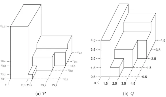
2.1 An arbitrary 3-dimensional orthogonal polytope P and its trans-formation Q . . . 11 2.2 Conflicting edges in the unit distance graph of R in Example 2 . . 23 2.3 Subgraphs of unit distance graph of R in Example 2 for Algorithm 2 24 4.1 Matrices forming x in HTD format for d“ 8. . . 57 4.2 Matrices forming x in HTD format for d_{“ 5. . . .} 58 4.3 Ranks of basis and transfer matrices forming πpitq_{, availability d}_{“ 8 70} 4.4 Densities of basis and transfer matrices forming πpitq_{, availability}

d_{“ 8 . . . .} 70 5.1 Maximum ranks of solution vectors for metabolite synthesis model 91 5.2 Maximum ranks of solution vectors for extended toggle switch model 93 5.3 Maximum ranks of solution vectors for lambda phage model . . . 95 5.4 Maximum ranks of solution vectors for cascade model with five

proteins . . . 97 5.5 Maximum ranks of solution vectors for cascade model with six

(13)

List of Tables

2.1 Properties of models from literature . . . 26

2.2 Experimental results for models from literature when states are processed in lexicographical order . . . 27

2.3 Experimental results for models from literature when states are processed in random order . . . 28

2.4 Properties of random test problems . . . 32

2.5 Experimental results for random test problems . . . 33

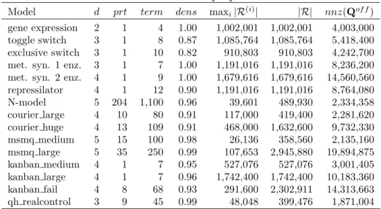
3.1 Model properties . . . 49

3.2 Numerical results (cont’d) . . . 51

4.1 Properties of availability and polling models . . . 66

4.2 Numerical results for availability models . . . 68

4.3 Numerical results for polling models . . . 69

5.1 Transition classes of metabolite synthesis model . . . 89

5.2 Numerical results for metabolite synthesis model . . . 90

5.3 Transition classes of extended toggle switch model . . . 91

5.4 Numerical results for extended toggle switch model . . . 92

5.5 Transition classes of lambda phage model . . . 93

5.6 Numerical results for lambda phage model . . . 94

5.7 Transition classes of cascade model five molecules . . . 95

5.8 Numerical results for cascade model with five molecules . . . 96

5.9 Transition classes of cascade model with six molecules . . . 97

(14)

LIST OF TABLES _xiv

(15)

Chapter 1 Introduction

The behavior of a physical system can be described by the states that the system may visit and how transitions from one state to another occur. The system can be modeled as a Markovian process if it exhibits the Markov property, that is, the future evolution of the system depends only on the current state of the system and not on the history of the process. A Markovian process with discrete state space is referred to as a Markov chain (MC). The Markov property requires that the time spent in a state of a MC during a visit exhibit the memoryless property, that is, time until the next transition does not depend on the time already spent in that state. The memoryless property dictates that the time spent in a state during a visit be exponentially distributed in a continuous-time MC (CTMC).

A CTMC can be represented by an _{p|S| ˆ |S|q real matrix Q, known as the} infinitesimal generator matrix, where S denotes the possibly countably infinite state space of the CTMC. The off-diagonal entries of Q are nonnegative and indicate the rates at which transitions occur. Specifically, Qpx, yq denotes the rate at which a transition occurs from state x to state y for x ‰ y. The di-agonal of Q is defined as the negated row sums of its off-didi-agonal entries (i.e., Q_{px, xq “ ´}ř

y‰xQpx, yq) Throughout our discussion, we assume that the tran-sition rates do not depend on time, that is, the CTMC is time-homogeneous. Time-inhomogeneous CTMCs are not in the scope of this thesis.

(16)

Let πt denote the transient probability distribution vector at time t ě 0. By definition, πthas |S| nonnegative entries and

ř

xπtpxq “ 1, where πtpxq denotes the probability of the system being in state x at time t _{ě 0. The system of} ordinary differential equations (ODEs) that describes the time evolution of the CTMC is given by

Bπt

Bt “ πtQ with initial condition πt ˇ ˇ ˇ t“0 “ π0. (1.1) It follows that πt “ π0eQt “ π0 8 ÿ i“0 pQtqi i! .

There are several numerical techniques to compute the transient probability vec-tor such as uniformization, ODE solvers, and Krylov subspace methods. When the state space is countably infinite, a CTMC obtained by truncating the state space is analyzed to approximate the transient distribution.

The limiting distribution

π _{“ lim}tÑ8πt

exists for some processes. This limit is referred to as the steady-state probability distribution and satisfies

πQ_{“ 0 and} ÿ

x

π_{pxq “ 1.}

Hence, π is a stationary distribution. The stationary distribution of a finite CTMC exists if and only if the CTMC is irreducible, i.e., each state is reachable from every other state. The existence of the stationary distribution of a countably infinite CTMC depends on the transition rates in the generator matrix as well as reachability. As for the transient analysis, the solution of the countably infinite CTMC can be computed by choosing a sufficiently large truncated state space.

Systems are usually composed of interacting subsystems. Such a system can be modeled as a multi-dimensional CTMC with each dimension of the CTMC rep-resenting a different subsystem and a number of events that trigger state changes at certain transition rates. In Kronecker-based Markovian modeling formalisms such as Stochastic Automata Networks (SANs) [129, 130], the set of rows and the

(17)

set of columns of the generator matrix are each equal to the product state space and the generator matrix is expressed as a sum of Kronecker products of subsys-tem transition matrices. In order to avoid unnecessary floating-point operations (flops) due to unreachable states, an auxiliary flag vector as long as the prod-uct state space can be used to indicate the reachability of states. However, this approach poses considerable inefficiency due to indexing and addressing during analysis when the reachable state space is significantly smaller than the product state space.

Compact storage of the generator matrix underlying a MC with no unreachable states and efficient implementation of analysis methods using Kronecker opera-tions require the reachable state space to be represented as a union of Cartesian products of subsets of subsystem state spaces [43] as it has been done, for instance, in hierarchical Markovian models (HMMs) [19]. Consequently, the generator ma-trix can be expressed as a block mama-trix in which the set of rows and columns corresponding to each diagonal block are the same, each set equals to a particu-lar partition of the reachable state space, and each block is a sum of Kronecker products of subsystem transition submatrices.

1.1 Kronecker Representation

Letting A_{P R}mAˆnA and BP RmBˆnB be two rectangular matrices, the Kronecker

(or tensor) product [42, 110] of A and B, i.e., A_{bB, yields the rectangular matrix} CP RmAmBˆnAnB _{whose entries satisfy}

C_pxC, yCq “ ApxA, yAqBpxB, yBq

with xC “ xAmB` xB and yC “ yAnB` yB for

pxA, yAq P t0, . . . , mA´ 1u ˆ t0, . . . , nA´ 1u , pxB, yBq P t0, . . . , mB´ 1u ˆ t0, . . . , nB´ 1u .

(18)

Note that the Kronecker product is associative; hence, it is defined for more than two matrices.

We consider a Markovian process _{tXptq “ pX}1ptq, . . . , Xdptqq P ˆd_h“1Sh, tě 0u associated with the d-dimensional CTMC, where Sh denotes the state space of dimension h _{“ 1, . . . , d. We assume that S}h are defined on consecutive nonneg-ative integers starting from 0. Otherwise, it is always possible to enumerate the subsystem state spaces so that they satisfy this assumption. The reachable state space R can be partitioned into the sets Rp1q, . . . , RpLq (i.e., R “ YL

l“1Rplq and Rplq_{X R}pl1_q

“ H for l ‰ l1_{), where R}plq

h Ď Sh consists of consecutive integers and Rplq _{“ ˆ}d

h“1R plq

h for l “ 1, . . . , L. Then, the infinitesimal generator Q can be viewed as an _{pL ˆ Lq block matrix induced by the partitioning tR}p1q_{, . . . , R}pLq_u as in Q_“ » — — – Qp1,1q _{. . .} _Qp1,Lq .. . . .. ... QpL,1q _{. . .} _QpL,Lq fi ffi ffi fl .

Block _{pl, l}1_{q of Q for l, l}1 _{“ 1, . . . , L is given by} Qpl,l1q _“ # ř jPTpl,l1qS pl,l1_q j ´ řL l1_“1 ř jPTpl,l1qD pl,l1_q j if l “ l1, ř jPTpl,l1qS pl,l1_q j otherwise, where Spl,l_j 1q _{“ ψ}j d â h“1 Spl,l_l,h1q, Dpl,l_j 1q _{“ ψ}j d â h“1 diag_pSpl,l_j,h1qe_q, ψj is the rate associated with transition j, Tpl,l

1_q

is the set of transitions in block pl, l1_{q, e represents a column vector of ones, and S}pl,l1q

j,h is the submatrix of the transition matrix Sj,h whose row and column state spaces are Rplq_h and Rpl

1_q

h , respectively. In practice, the matrices Sj,h are sparse and held in sparse row format since the nonzeros in each of its rows indicate the possible transitions from the state with that row index.

Throughout the thesis, calligraphic uppercase letters are used for sets. Vectors and matrices are respectively represented with boldface lowercase and boldface uppercase letters. All vectors are row vectors except e and eh which represent a column vector of ones and the hth column of the identity matrix, respectively.

(19)

1 denotes a row vector of ones and Im denotes the identity matrix of order m. Lengths of vectors are determined from the contexts in which they are used. Order of an identity matrix is determined from the context if its subscript is omitted. diagpaq denotes the diagonal matrix with the entries of vector a along its diagonal. nnz_{pAq denotes the number of nonzeros in A. ApX , Yq is the} submatrix of A where rows and columns are respectively selected from sets X and Y, and A_{px, yq is the value of the matrix A corresponding to element px, yq.} Consistently, a_{pxq is the value of the vector a at state x and apX q is the subvector} of a including the values of a_{pxq for x P X . Z, Z}ě0, Rě0 and Rą0 stand for sets of integers, nonnegative integers, nonnegative real numbers, and positive real numbers, respectively. O_{p¨q stands for the big O notation. The complexities of} the algorithms are worst case complexities unless otherwise stated. Finally, T_, | ¨ |, ˆ, b, and ‹ respectively denote transposition, the number of elements in a set, Cartesian product operator, Kronecker product operator, and elementwise multiplication operator.

1.2 Layout of the Thesis

Representing the reachable state space as a union of Cartesian products of sub-sets of subsystem state spaces is essential to store the generator matrix compactly and implement efficient analysis methods using Kronecker operations. The next chapter, which is based on [51], shows that the problem of partitioning the reach-able state space of a three or higher dimensional system with a minimum number of partitions into Cartesian products of subsets of subsystem state spaces is NP-complete. Then it presents two algorithms that can be used to compute possibly non-optimal partitionings of a given reachable state space and investigates the performance of these algorithms through a set of problems from the literatue and those that are randomly generated.

The generator matrix is not explicitly generated when it is represented com-pactly using Kronecker products. The implementation of efficient transient and steady-state solvers rests on efficient vector–Kronecker product multiplication

(20)

algorithms such as the shuffle algorithm. Chapter 3, which is based on [49], im-proves the shuffle algorithm by omitting zero rows and columns in the factors of the Kronecker product terms that result in unnecessary (flops) and shows the effectiveness of the modification through a set of problems from the literature.

The Kronecker representation of the generator matrix decreases the memory requirement; however, solution vectors used in the analysis still require to be as long as the size of the reachable state space. Chapter 4, which is based on [29], shows that it is possible to use the hierarchical Tucker decomposition (HTD) to store the solution vectors and still carry out the basic operation of vector–matrix multiplication in Kronecker form relatively efficiently.

Chapter 5 considers a stochastic chemical system modelled as a CTMC with a countably infinite multi-dimensional state space and solves the system of ODEs that describes the time evolution of the CTMC by a backward differentiation formula with vectors in HTD format. Numerical experiments indicate that adap-tive truncation strategies improve time and memory efficiency significantly when fixed truncation strategies are inefficient.

Chapter 6, which is based on [53], considers a multi-class retrial queueing sys-tem with acyclic PH retrials. A necessary and sufficient condition for ergodicity is obtained from criteria based on drifts. The countably infinite state space of the model is truncated with an appropriately chosen Lyapunov function. The truncated model is described as a multi-dimensional MC and a Kronecker repre-sentation of its generator matrix is numerically analyzed.

(21)

Chapter 2 Cartesian product partitioning

A d-dimensional orthogonal polytope can be represented by a set of d-dimensional vectors [16]. In such a representation, the Cartesian product of sets of consecu-tive integers represents a hyper-rectangle. Hence, Cartesian product partitioning of a d-dimensional reachable state space is equivalent to the hyper-rectangular partitioning of the d-dimensional polytope that is represented by the reachable state space. Partitioning a 2-dimensional orthogonal polytope into a minimum number of hyper-rectangles is well studied and there are polynomial time algo-rithms for this problem [69, 98, 143]. However, the 3-dimensional version of this problem is shown to be NP-complete [59]. In [96], an algorithm to partition a 3-dimensional orthogonal polytope into hyper-rectangles is proposed. To the best of our knowledge, there is no algorithm to partition a d-dimensional orthogonal polytope into hyper-rectangles for d_{ą 3.}

Our motivation is to automate the partitioning of a given multi-dimensional reachable state space into Cartesian products of subsets of subsystem state spaces. For practical purposes, the number of partitions in the partitioning should be kept as small as possible. With this objective in mind, we first show that the problem of partitioning the reachable state space of a three or higher dimensional system with a minimum number of partitions into Cartesian products of subsets of subsystem state spaces is NP-complete [72]. Then we present two algorithms

(22)

that can be used to compute possibly non-optimal partitionings of the reachable state space into Cartesian products of subsets of subsystem state spaces.

The first algorithm starts with partitions as singletons, each representing a reachable state. Two partitions are merged if their union is also a Cartesian product of sets of consecutive integers. The partitions are merged until there are no partitions that can be merged with each other. We call this the merge based algorithm. The second algorithm takes a different approach. First, the unit distance graph of the reachable state space is constructed. The vertex set of this graph is the reachable state space and there is an edge between two vertices if the distance between them is one. Then this graph is refined [125] by removing edges until no further refinement is necessary. We call this the refinement based algorithm.

Through a set of problems from the literature [21, 26, 30] and those that are randomly generated, the performance of the two algorithms is investigated. Re-sults indicate that although it may be more time and memory consuming, the refinement based algorithm almost always computes partitionings with a smaller number of partitions than the merge based algorithm. In many cases, the par-titionings computed by the refinement based algorithm are the optimal ones. Furthermore, the refinement based algorithm is insensitive to the order in which the states in the reachable state space are processed.

The next section introduces the notation and preliminary definitions used. The second section defines the partitioning problem formally, shows that it is NP-complete, and presents two algorithms that provide, possibly non-optimal, solutions to the problem. The third section reports on experimental results with the two algorithms.

(23)

2.1 Notation and definitions

A d-dimensional hyper-rectangle is defined to be a Cartesian product of d intervals as in _ˆd

h“1rah, bhs, where rah, bhs Ď R is an interval for ah ă bh, ah, bh P R, and h_{“ 1, . . . , d. A point set X Ď R}d _{is convex if the line segment between x and y} is in X for x, y _{P X . The convex hull of X is the smallest set containing X . A} d-dimensional convex polytope is the convex hull of a finite set X _{Ď R}d _{[153]. A} d-dimensional polytope is the union of a finite number of d-dimensional convex polytopes. A d-dimensional polytope is orthogonal if it is a union of d-dimensional hyper-rectangles [16].

Let G _{“ pV, Eq be an undirected graph with vertex set V and edge set E. A} graph G1 _{“ pV}1_{, E}1_{q is a subgraph of G “ pV, Eq if V}1 _{Ď V and E}1 _{Ď tpx, yq P} E | x, y P V1_{u. A subgraph of G “ pV, Eq induced by V}1 _{Ď V is a graph whose} vertex set is V1 _{and edge set is}_{tpx, yq P E | x, y P V}1_{u. Two vertices of a graph are} said to be connected if there exists a sequence of edges that lead from one of the vertices to the other. A subgraph of G_{“ pV, Eq forms a connected component if} each pair of vertices in the subgraph are connected. A unit distance graph is a graph having a drawing in which all edges are of unit length [114].

2.2 Cartesian product partitioning algorithms

We are interested in partitionings, where the partitions themselves are Cartesian products of subsets of subsystem state spaces. Next we define the Cartesian product partitioning problem.

Definition 1. The set _tRp1q_{, . . . , R}pLq_{u is said to be a Cartesian product} par-titioning of the multi-dimensional reachable state space R if Rplq _{“ ˆ}d

h“1R plq h , the state space of the hth subsystem Rplq_h _{Ď S}h consists of consecutive integers, YL

l“1Rplq “ R, and RplqX Rpl

1_q

“ H for h “ 1, . . . , d, l ‰ l1_{, l, l}1 _{“ 1, . . . , L, and} L_{P Z}ą0.

(24)

For practical purposes that aid the use of Kronecker operations, the number of partitions in the Cartesian product partitionings of R should be as small as possible. Therefore, our interest lies in minimizing the number of partitions in the partitioning of R. Unfortunately, the decision problem derived from the minimum Cartesian product partitioning problem is NP-complete [72] when the system has three or higher dimensions as we next show.

Theorem 1. It is NP-complete to decide whether there is a Cartesian product partitioning of the multi-dimensional reachable state space R with less than LR partitions for given d_{P Z}ą0, LRP Zą0, and RĎ Zdě0 when dě 3.

Proof. It is possible to check whether a set of states is a Cartesian product of sets of consecutive integers, two sets are disjoint, and the union of given sets is equal to R in polynomial time. Therefore, the Cartesian product partitioning problem is in class NP.

For a given arbitrary d-dimensional orthogonal polytope P _{Ď R}d_{and an integer} LR P Zą0, it is NP-complete to decide whether P can be partitioned into LR or less d-dimensional hyper-rectangles for d ě 3 since it is NP-complete when instances are restricted to d_{“ 3 [59]. Now, let V Ď P be the vertex set of P and} V_h _{“ tx}_h _{P R | x “ px}₁_{, . . . , x}_d_{q P Vu for h “ 1, . . . , d. Furthermore, assume that} the elements of Vh “ tvh,1, . . . , vh,|Vh|u are ordered so as to satisfy vh,l ă vh,l1 if

and only if l_{ă l}1 _{for l, l}1 _{“ 1, . . . , |V}

h| and h “ 1, . . . , d.

Since P is an orthogonal polytope, there exists LP Zą0 such that P “ L ď l“1 ˆd h“1ra plq h , b plq h s, where _ˆd h“1ra plq h , b plq

h s is a hyper-rectangle for l “ 1, . . . , L. Note that P can be transformed to an orthogonal polytope Q _{Ď R}d _{(see Figure 2.1) for which the} minimum hyper-rectangular partitionings of P and Q include the same number of hyper-rectangles as we next show.

(25)

(a) P (b) Q

Figure 2.1: An arbitrary 3-dimensional orthogonal polytope P and its transfor-mation Q Let fhpxhq “ # l_{´ 0.5 ` g}hpxhq if vh,1 ď xh ă vh,|Vh| |Vh| ´ 0.5 if xh “ vh,|Vh|

be the transformation function, where

ghpxhq “ pxh ´ vplq_h q{pvpl`1q_h ´ v_dplkqq

for xh P rvh,l, vh,l`1q, l “ 1, . . . , |Vh| ´ 1, and h “ 1, . . . , d. The function fh : rvh,1, vh,|Vh|s Ñ r0.5, |Vh|´0.5s is continuous and increasing, so the transformation

of an interval is also an interval, that is,

tyh P R | xh P rah, bhs, yh “ fhpxhqu “ rfhpahq, fhpbhqs. Then the set

Q “ ty P Rd | x P P, yh “ fhpxhq for h “ 1, . . . , du “ ty P Rd | x P YLl“1ˆ d h“1ra plq h , b plq h s, yh “ fhpxhq for h “ 1, . . . , du “ L ď l“1 ˆd h“1rfhpa plq h q, fhpb plq h qs

is an orthogonal polytope since it is a union of hyper-rectangles, and rfhpxplqh q, fhpbplqh qs X rfhpapl

1_q

h q, fhpbpl

1_q

(26)

holds if raplqh , b plq h s X ra pl1_q h , b pl1_q h s “ H for l ‰ l1, l, l1 “ 1, . . . , L, and h “ 1, . . . , d. Therefore, if P can be partitioned into L hyper-rectangles, then Q can be par-titioned into L or less hyper-rectangles. The inverse of the function fh is also increasing and continuous. Hence, Q can be transformed to P similarly. So, we conclude Q can be partitioned into L hyper-rectangles if and only if P can be partitioned into L hyper-rectangles.

Now, we transform the orthogonal polytope Q to the d-dimensional reachable state space, R. Each vertex v _{“ pv}1, . . . , vdq of Q satisfies vh ´ 0.5 P Zě0 for h_{“ 1, . . . , d, so} Q “ M ď m“1 ˆdh“1rx pmq h ´ 0.5, x pmq h ` 0.5s, where _txp1q, . . . ,xpM q_{u “ Q X Z}d ě0 for some M P Zą0 [16]. Let R_{“ Q X Z}d

ě0 andtRp1q, . . . , RpLqu be a Cartesian product partitioning of R, where Rplq_{“ ˆ}d

h“1R plq

h for l“ 1, . . . , L. Then Q can be written as a union of disjoint hyper-rectangles, that is,

Q “ ď xPR ˆd h“1rxh´ 0.5, xh` 0.5s “ L ď l“1 ˆdh“1rminpR plq h q ´ 0.5, maxpR plq h q ` 0.5s.

Therefore, if R can be partitioned into L Cartesian products of sets of consecutive integers, then Q can be partitioned into L or less hyper-rectangles.

Now, let _tQp1q_{, . . . , Q}pLq_{u be a hyper-rectangular partitioning of Q, where} Qplq _{“ ˆ}d h“1ra plq h , b plq h s for l “ 1, . . . , L. Then R “ L ď l“1 pQplqX Zd ě0q “ L ď l“1 ˆd h“1pra plq h , b plq h s X Zě0q,

where _raplq_h , bplq_h _{s X Z}ě0 is a set of consecutive integers if it is not empty for l “ 1, . . . , L and h_{“ 1, . . . , d. Besides, R}plq_{X R}pl1_q

“ H for l ‰ l1 _{and l, l}1 _{“ 1, . . . , L.} Then_tRp1q_{, . . . , R}pLq_{u is a Cartesian product partitioning of R. Therefore if Q can} be partitioned into L hyper-rectangles, then R can be partitioned into L or less Cartesian products of sets of consecutive integers. Thus, R can be partitioned

(27)

into L partitions if and only if Q can be partitioned into L hyper-rectangles. Therefore, R can be partitioned into less than LR partitions if and only if P can be partitioned into less than LR hyper-rectangles. Then it is NP-complete to compute the Cartesian product partitioning of R Ď Zd

ě0 with less than LR partitions.

Now, we present two algorithms to compute Cartesian product partitionings of the multi-dimensional reachable state space R. The first algorithm starts with partitions as singletons, each representing a reachable state. A partition is merged with another partition if their union is also a Cartesian product of sets of consecutive integers. This algorithm terminates when there are no partitions that can be merged with each other. The second algorithm takes a different approach. The unit distance graph of the reachable state space is constructed. Then this graph is refined by removing edges until the vertex set of each connected component can be expressed as a Cartesian product of sets of consecutive integers.

2.2.1 Merge based partitioning

We start by defining set mergeability and then provide the condition for the mergeability of two partitions in a Cartesian product partitioning of R.

Definition 2. Let X _{“ ˆ}d

h“1Xhand Y “ ˆd_h“1Yhbe two partitions in a Cartesian product partitioning of R. The partitions X and Y are said to be mergeable if X _{Y Y “ ˆ}d

h“1pXh Y Yhq and Xh Y Yh consists of consecutive integers for h_{“ 1, . . . , d.}

Lemma 1. Let X _{“ ˆ}d

h“1Xh and Y “ ˆdh“1Yh be two partitions in a Cartesian product partitioning of R. The partitions X and Y are mergeable if and only if there exists some i_{“ 1, . . . , d such that maxpX}iq ` 1 “ minpYiq or maxpYiq ` 1 “ min_pXiq, and Xh “ Yh for h“ 1, . . . , i ´ 1, i ` 1, . . . , d.

(28)

and Xh “ Yh for h“ 1, . . . , i ´ 1, i ` 1, . . . , d. Then X Y Y “ `ˆd h“1Xh˘ ď `ˆdh“1Yh ˘ “ `pî´1 h“1Xhq ˆ Xi ˆ pˆd_h“i`1Xhq ˘ ď `pî´1 h“1Yhq ˆ Yiˆ pˆdh“i`1Yhq ˘ “ `pî´1 h“1pXhY Yhqq ˆ Xiˆ pˆdh“i`1pXhY Yhqq ˘ ď `pî´1 h“1pXhY Yhqq ˆ Yiˆ pˆd_h“i`1pXhY Yhqq ˘ “ pî´1h“1pXhY Yhqq ˆ pXiY Yiq ˆ pˆdh“i`1pXhY Yhqq “ ˆd h“1pXhY Yhq

holds. The set XhY Yh consists of consecutive elements for h“ 1, . . . , d. Hence, X and Y are mergeable partitions.

pñq Let X Ď R and Y Ď R be disjoint mergeable partitions. We first show that there exists i_{“ 1, . . . , d such that X}iX Yi “ H. Assume that XhX Yh ‰ H for h_{“ 1, . . . , d. Then there exists u “ pu}1, . . . , udq P S such that uh P XhXYhfor h_{“ 1, . . . , d. However, this contradicts the assumption that X and Y are disjoint.} Thus XiX Yi “ H for some i “ 1, . . . , d. Besides, either maxpXiq ` 1 “ minpYiq or max_pYiq ` 1 “ minpXiq holds since XiY Yi consists of consecutive elements.

Now we show that Xh “ Yh for h “ 1, . . . , i ´ 1, i ` 1, . . . , d. For the sake of contradiction, suppose there exists j _{“ 1, . . . , i ´ 1, i ` 1, . . . , d such that} X_j _{‰ Y}_j (i.e., _pXjzYjq Y pYjzXjq ‰ H). Without loss of generality, assume that XjzYj ‰ H. Then there exists u “ pu1, . . . , udq P ˆd_h“1pXh Y Yhq, where ui P YizXi and uj P XjzYj. Therefore, uR X Y Y since ui R Xi and uj R Yj. Then X Y Y ‰ ˆd

h“1pXhY Yhq holds, but this contradicts the assumption that X and Y are mergeable partitions. Therefore Xh “ Yh for h“ 1, . . . , i ´ 1, i ` 1, . . . , d.

Now, we demonstrate the concept of mergeability on an example.

Example 1. Let d_{“ 3, S}h “ t0, 1, 2u for h “ 1, 2, 3, and let X “ t0, 1uˆt1uˆt2u be a partition in a Cartesian product partitioning of some R _{Ď ˆ}3

h“1Sh. Then by Lemma 1, the partitions that can be merged with X are _{t2u ˆ t1u ˆ t2u,} t0, 1u ˆ t0u ˆ t2u, t0, 1u ˆ t2u ˆ t2u, t0, 1u ˆ t1u ˆ t1u, and t0, 1u ˆ t1u ˆ t0, 1u.

(29)

Let X _{“ ˆ}d

h“1Xh be a partition in a Cartesian product partitioning of R. The states _pminpX1q, . . . , minpXdqq P X and pmaxpX1q, . . . , maxpXdqq P X are said to be the end states of the partition X . Due to Lemma 1, mergeability of two partitions can be determined by their end states. Besides, the states in a partition can be obtained from its end states. Therefore, it is sufficient to keep only the end states of the partitions instead of maintaining the partitions by using a disjoint-set data structure and a union-find algorithm [41] to merge two partitions.

Input: d-dimensional reachable state space: R Output: Cartesian product partitioning of R: Q

1: function MergeBasedPartitioning(R, Q) 2: Q Ð H

3: for all xP R do 4: X Ð txu

5: whilethere exists some YP Q mergeable with X do 6: X Ð X Y Y; Q Ð QztYu

7: end while 8: Q Ð Q Y tX u 9: end for

10: end function

Algorithm 1: Merge based algorithm to compute a Cartesian product parti-tioning of given multi-dimensional reachable state space

In Algorithm 1, we provide the merge based Cartesian product partitioning of R. It starts by constructing a singleton for each state in R. For each partition that is a singleton or is obtained by merging two partitions, a mergeable partition is sought. If such a partition is located, the two partitions are merged. There are |R| partitions; hence, the total time complexity of constructing a new partition is O_{pd|R|q. A new partition is obtained when a singleton is constructed or two} partitions are merged. Initially there are _{|R| partitions, and the partitions in} the partitioning never get split, implying there can be at most _{p|R| ´ 1q merge} operations. Then the total cost of merging two partitions is O_{pd|R|q. Since each} partition needs to check O_{pdq end states for mergeability with another partition,} a mergeable partition is sought O_{pd|R|q times.}

The efficiency of the algorithm depends on the data structure used to keep the end states of the partitions. When a balanced tree such as an AVL tree [4] is used to keep the end states, the cost of searching for a partition becomes O_plgpLmaxqq

(30)

time, where Lmax is the maximum number of partitions during the execution of the algorithm. Therefore, the time complexity of the algorithm associated with seeking a mergeable partition is O_{pd|R| lgpL}maxqq when the end states of the partitions are kept in a balanced tree. Another cost in the algorithm is inserting end states to the tree when no mergeable partition is found and removing the end states from the tree when two partitions are merged. The time complexities of these operations are also O_{p|R| lgpL}maxqq. Therefore, the time complexity of the algorithm is O_{pd|R| lgpL}maxqq. The space requirement for each partition is Opdq; hence, the space requirement of the algorithm is O_pdLmaxq. In the worst case, no partitions are merged and Lmax “ |R|; hence, the time and space complexities of the algorithm are O_{pd|R| lgp|R|qq and Opd|R|q, respectively. If L}max is constant, the number of partitions is bounded by a constant during the execution of the algorithm. In that case, the time and space complexities of the algorithm become O_{pd|R|q and Opdq, respectively.}

Observe that the partition computed by Algorithm 1 depends on the order in which the states of R are processed. Now, let us consider the following 3-dimensional example.

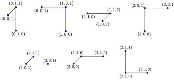
Example 2. Let Sh “ t0, 1, 2, 3u for h “ 1, 2, 3,

R “ tp0, 0, 1q, p0, 1, 0q, p0, 1, 1q, p1, 0, 0q, p1, 0, 1q, p1, 1, 0q, p1, 1, 1q, p2, 0, 0q, p2, 0, 1q, p2, 1, 0q, p2, 1, 1q, p3, 0, 1q, p3, 1, 0qu,

and assume that the states in R are processed in lexicographical order.

When the first 8 states are processed, the partitions are _{tp0, 0, 1q, p0, 1, 1qu,} tp1, 1, 1qu, tp0, 1, 0q, p1, 1, 0qu, tp1, 0, 0q, p1, 0, 1qu, and tp2, 0, 0qu. Then the single-ton _{tp2, 0, 1qu is merged with the singleton tp2, 0, 0qu, and their union is merged} with _{tp1, 0, 0q, p1, 0, 1qu. Finally, the remaining states are processed.}

The number of partitions in the Cartesian product partitioning of R turns out to be 5, and the partitions are given by tp0, 1, 0q, p1, 1, 0q, p2, 1, 0q, p3, 1, 0qu, tp1, 1, 1q, p2, 1, 1qu, tp0, 0, 1q, p0, 1, 1qu, tp1, 0, 0q, p1, 0, 1q, p2, 0, 0q, p2, 0, 1qu, and tp3, 0, 1qu.

(31)

2.2.2 Refinement based partitioning

The refinement based partitioning algorithm constructs the unit distance graph of the multi-dimensional reachable state space R. The vertex set of this graph is R and there is an edge between two vertices x, y P R if x ´ y P Yd

h“1t´eh,ehu. In other words, two vertices are adjacent in the unit distance graph if there is consecutiveness of the vertices along a particular dimension while the values of states variables in other dimensions remain constant. We next define conflicting edges in a subgraph of the unit distance graph.

Definition 3. Let G _{“ pR, Eq be a subgraph of the unit distance graph of R} and let x, x_{` δ}i,x` δj P R for some i, j “ 1, . . . , d, i ‰ j, δi P t´ei,eiu, and δj P t´ej,eju. Two edges px, x ` δiq, px, x ` δjq P E are said to be conflicting if x_{` δ}i` δj R R or tpx ` δi,x` δi` δjq, px ` δj,x` δi` δjqu Ę E.

The next lemma and corollary show that in a subgraph of the unit distance graph of R with no conflicting edges, the vertices in each connected component can be written as a Cartesian product of sets of consecutive integers. Therefore, eliminating conflicting edges in the unit distance graph of R leads to a Cartesian product partitioning of R.

Lemma 2. Let G_{“ pR, Eq be a subgraph of the unit distance graph of R with} no conflicting edges, M _{P Z}ą0, xpmq “ pxpmq1 , . . . , x pmq d q P R for m “ 0, . . . , M, and X pMq “ ˆd h“1t M min m“0px pmq h q, . . . , M max m“0px pmq h qu.

If _pxpm´1q_,_xpmq_{q P E for m “ 1, . . . , M, then X pMq Ď R and pu, vq P E for} u_{´ v P Y}d

h“1t´eh,ehu and u, v P X pMq.

Proof. The proof is by mathematical induction on m. The base case is trivial. Assume that the statement holds when pxpm´1q_,_xpmq_{q P E for m “ 1, . . . , M ´ 1.} Now, let _pxpM ´1q_,_xpM q_{q P E. If X pMqzX pM ´ 1q “ H, the statement holds by}

(32)

the inductive hypothesis. Otherwise, X pMqzX pM ´ 1q “ ˆ ˆi´1 h“1t M´1 min m“1px pmq h q, . . . , M´1 max m“1px pmq h qu ˙ ˆ txpM ´1qi ` δu ˆ ˆ ˆdh“i`1t M´1 min m“1px pmq h q, . . . , M´1 max m“1px pmq h qu ˙

is not empty, where δ _{“ x}pM q_i _{´ x}pM ´1q_i _{P t´1, 1u for some i “ 1, . . . , d. Let} Y “ ty P X pMqzX pM ´ 1q | y R R or py, y ´ δeiq R Eu

and assume that Y ‰ H. Then there exists x, y P X pMqzX pM ´ 1q such that x_{R Y, y P Y, and x ´ y P Y}d

h“1t´eh,ehu. In this case, px ´ δei,y´ δeiq P E by the inductive hypothesis and _{px, x ´ δe}iq P E since x R Y. Then px, x ´ δeiq and px ´ δei,y´ δeiq are conflicting edges in G, but this contradicts the assumption that G does not contain conflicting edges. Hence, Y _{“ H, that is, u P R and} pu, u ´ δeiq P E for u P X pMqzX pM ´ 1q. Now, let x, y P X pMqzX pM ´ 1q be two arbitrary vertices such that x´y P Yd

h“1t´eh,ehu. Since Y “ H, tx, yu Ď R and

tpx, x ´ δeiq, py, y ´ δeiq, px ´ δei,y´ δeiqu Ď E.

Thenpx, yq P E since there are no conflicting edges in G. Therefore, the statement also holds for M.

Corollary 1. Let G _{“ pR, Eq be a subgraph of the unit distance graph of R} with no conflicting edges and G1 _{“ pR}1_{, E}1_{q be a connected component in G.} Then R1 _{can be written as a Cartesian product of consecutive integers, that is,} R1 _{“ ˆ}d

h“1tuh, . . . , vhu, where u “ pu1, . . . , udq P R, v “ pv1, . . . , vdq P R, and uh ď vh for h“ 1, . . . , d.

The next definition introduces the concept of a separator, which is used in refining the unit distance graph of R.

Definition 4. Let U, V _{Ď R and G “ pR, Eq be a subgraph of the unit distance} graph of R. The set of edges Z Ď E is said to be a separator if

(33)

2. subgraphs of G induced by the sets U and V are each connected,

3. there does not exist two vertices x, y _{P R such that px, x ` δe}hq P Z, py, y ` δehq P EzZ, tpx, yq, px ` δeh,y` δehqu Ď E, and

4. there exists at least one edge in Z that conflicts with some edge in E,

where U Ď tx P R | xh “ iu and V Ď tx P R | xh “ i ` δu for some i P Sh, δ_{P t´1, 1u, and h “ 1, . . . , d.}

The next lemma shows that removing the edges in a separator decreases the number of conflicting edges in a subgraph of the unit distance graph of R. Lemma 3. Let G “ pR, Eq be a subgraph of the unit distance graph of R and Z be a separator in G. Two edges in G1 _{“ pR, EzZq conflict only if they also} conflict in G.

Proof. Let_{px, x`δ}iq and px, x`δjq be two edges that do not conflict in G for some i, j _{“ 1, . . . , d, i ‰ j, δ}i P t´ei,eiu, and δj P t´ej,eju. Then x ` δi` δj P R and tpx`δi,x`δi`δjq, px`δj,x`δi`δjqu Ď E. Due to Definition 4, px, x`δiq P Z if and only if _{px ` δ}j,x` δi` δjq P Z. Similarly, px, x ` δjq P Z if and only if px ` δi,x` δi` δjq P Z. Then,

tpx ` δi,x` δi` δjq, px ` δj,x` δi` δjqu Ď EzZ

if_{tpx, x`δ}iq, px, x`δjqu Ď EzZ. Therefore, if the two edges in G do not conflict, then they do not conflict in G1_.

Now, we are in a position to provide the refinement based algorithm for Carte-sian product partitioning of R (see Algorithm 2). At the outset, the unit distance graph of R is constructed. Then the separators in this graph are constructed and inserted to a priority queue [41], where the priority of a separator is the total number of edges which conflict with an edge in the separator. The graph is re-fined by removing the separator with maximum priority until no conflicting edges remain. The edge set of the graph changes when a separator is removed; hence,

(34)

the separators need to be reconstructed. By Lemma 3, an edge is conflicting in the refined graph only if it is also conflicting before refinement. Hence, each sepa-rator in the refined graph is a subset of a sepasepa-rator in the graph before refinement. Therefore, in order to reconstruct the separators, it is necessary and sufficient to visit the vertices incident to the edges in the separators intersecting the removed separator, where two separators are said to be intersecting if they include edges along different dimensions incident to the same vertex. If all conflicting edges are eliminated, then the vertices in each connected component can be written as a union of Cartesian products of sets of consecutive integers by Corollary 1.

Input: d-dimensional reachable state space: R Output: Cartesian product partitioning of R: Q

1: function RefinementBasedPartitioning(R, Q) 2: Construct unit distance graph of R, G“ pR, Eq 3: Construct an empty priority queue PQ

4: for all xP R do

5: for allh“ 1, . . . , d do 6: if x` ehP R then

7: if px, x ` ehq conflicts with some edge in E

8: ANDpx, x ` ehq is not in a separator then

9: Construct separator Z includingpx, x ` ehq; Insert Z to PQ

10: end if 11: end if 12: end for 13: end for

Algorithm 2: Refinement based algorithm to compute a Cartesian product partitioning of given multi-dimensional reachable state space

In order to construct the unit distance graph, first all adjacent vertices need to be determined. In order to facilitate this, each vertex keeps an adjacency list of length 2d to identify the adjacent vertices. The vertices are first inserted to an AVL tree [4]. Then for each vertex, vertices that might be adjacent in the product state space are sought in the tree. There are 2d such vertices; hence, 2d vertices are sought for each vertex. Therefore, the space complexity of maintaining the graph becomes O_{pd|R|q and the time complexity of constructing the unit distance} graph becomes O_{pd|R| lgp|R|qq. After the graph is constructed, the AVL tree is} destroyed.

(35)

14: while PQis not empty do

15: ZmaxÐ separator Z in PQ whose priority is maximum

16: Remove Zmax from PQ

17: for allpx, yq P Zmaxdo

18: L Ð H

19: for allseparators Z in PQ including an edge incident to x or y do 20: L Ð L Y tZu; Remove Z from PQ

21: end for 22: end for 23: E Ð EzZmax

24: for all ZP L do 25: while Z‰ H do

26: Construct the separator Z1 _{including some edge}_{px, yq P Z; Z Ð ZzZ}1

27: if priority of Z1 _{is positive then}

28: Insert Z1 _{to PQ} 29: end if 30: end while 31: end for 32: end while 33: Q Ð H

34: for allconnected components G1 _{“ pR}1_{, E}1_{q of G “ pR, Eq do}

35: Q Ð Q Y tR1_u

36: end for 37: end function

Algorithm 2: Refinement based algorithm to compute a Cartesian product partitioning of given multi-dimensional reachable state space (cont’d)

Each separator includes at least one conflicting edge, that is, its priority is posi-tive. Algorithm 2 visits each edge and checks whether it conflicts with some other edge. A separator is formed by the two vertex sets (U and V in Definition 4) and the subgraphs induced by these two sets are connected. Besides, the separator is maximal; hence, the separator including a particular edge is unique and only one separator can include the edge (see Item 3 of Definition 4). Therefore, the separator including an edge is constructed only once in the unit distance graph. While constructing a separator Z including the edge_{px, yq, a breadth-first search} starting at x is used to visit the vertices connected to x [41]. The time complexity of constructing the separator Z is O_{pd|Z|q. Since each edge is added to at most} one separator, the number of edges in the union of separators is O_p|E|q. There-fore, the total time complexity of constructing all separators in the unit distance graph becomes Opd|E|q. At each vertex, we use an array of size 2d to keep the separators including the edge incident to that vertex. The space complexity of the algorithm remains as O_{pd|R|q, but it takes constant time to retrieve the separator}

(36)

including a given edge.

When a separator is constructed, it is added to the priority queue. We use a binary heap as the priority queue. Observe that the number of separators does not exceed_{|E| since each separator includes at least one edge. Therefore, the cost} of inserting separators to the priority queue is O_{p|E| lgp|E|qq. We consider an array} implementation of the priority queue and the maximum number of separators is not known in advance; therefore, we allocate O_{p|E|q “ Opd|R|q space for the} priority queue.

After the separators in the unit distance graph are inserted to the priority queue, the graph is refined by removing the edges in the separator with max-imum priority until no separators remain in the priority queue. The graph is refined at most _{|E| times since at least one edge is removed from the graph at} each refinement step. At each refinement step, the separator with maximum pri-ority, Zmax, is chosen. When Zmax is removed, the intersecting separators need to be reconstructed. Hence, at each refinement step, all edges of Zmax are visited to obtain the intersecting separators. These separators are inserted to a list L and removed from the heap. Then these separators are reconstructed for the edge set E zZmax and inserted to the heap. Reconstruction of a separator Z requires visit-ing all the vertices incident to the edges in it. The number of edges in the union of separators intersecting with Zmax is Opd|E|q; hence, reconstruction of separators at each step has time complexity O_{pd|E|q. Therefore, the total time complexity} of reconstructing separators becomes O_pd|E|2_{q since reconstruction is required in} all refinement steps. Now, consider the costs related to the heap operations. At each refinement step, the separators intersecting with Zmax are removed from the heap. The separator Zmax intersects with Opd|Zmax|q separators. Therefore, dur-ing the execution of the algorithm, the total number of removals from the heap is O_{pd|E|q since the total size of the separators removed from the graph is Op|E|q.} The algorithm starts and ends with an empty heap, so the number of insertions to the heap is also O_{pd|E|q. Hence, the total complexity of heap operations is} O_{pd|E| lgpd|E|qq. When all costs are considered, the time and space complexities} of Algorithm 2 are O_pd|E|2

q “ Opd3 |R|2

(37)

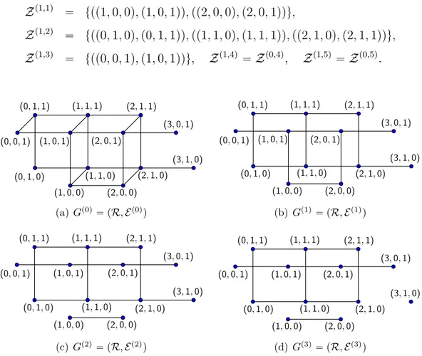
Example 2. (cont’d) Algorithm 2 first constructs the unit distance graph of R and then refines the graph by removing edges. Let Gpjq _{“ pR, E}pjq_{q denote} the subgraph of the unit distance graph of R, where Epjq _{is the edge set after j} separators are removed. In the unit distance graph of R, Gp0q_{, there are 7 pairs} of conflicting edges (see Figure 2.2).

Figure 2.2: Conflicting edges in the unit distance graph of R in Example 2 The separators in the unit distance graph of R (see Figure 2.3(a)) are

Zp0,1q “ tpp0, 0, 1q, p0, 1, 1qq, pp1, 0, 0q, p1, 1, 0qq, pp1, 0, 1q, p1, 1, 1qq, pp2, 0, 0q, p2, 1, 0qq, pp2, 0, 1q, p2, 1, 1qqu Zp0,2q _{“ tpp0, 1, 0q, p0, 1, 1qq, pp1, 0, 0q, p1, 0, 1qq, pp1, 1, 0q, p1, 1, 1qq,} pp2, 0, 0q, p2, 0, 1qq, pp2, 1, 0q, p2, 1, 1qqu Zp0,3q _{“ tpp0, 0, 1q, p1, 0, 1qq, pp0, 1, 0q, p1, 1, 0qq, pp0, 1, 1q, p1, 1, 1qqu} Zp0,4q _{“ tpp2, 0, 1q, p3, 0, 1qqu, Z}p0,5q_{“ tpp2, 1, 0q, p3, 1, 0qqu.}

The priorities of the separators Zp0,1q _{and Z}p0,2q _{are 4, and the priorities of the} other separators are 2. There are two separators with maximum priority and one of them needs to be chosen. Let the edges in Zp0,1q _{be chosen for removal. Then} all other separators are reconstructed and 3 conflicting edges remain in Gp1q _(see

(38)

Figure 2.3(b)). The separators in this graph are Zp1,1q _{“ tpp1, 0, 0q, p1, 0, 1qq, pp2, 0, 0q, p2, 0, 1qqu,} Zp1,2q “ tpp0, 1, 0q, p0, 1, 1qq, pp1, 1, 0q, p1, 1, 1qq, pp2, 1, 0q, p2, 1, 1qqu, Zp1,3q _{“ tpp0, 0, 1q, p1, 0, 1qqu, Z}p1,4q _{“ Z}p0,4q, Zp1,5q _{“ Z}p0,5q. (a) Gp0q_{“ pR, E}p0q_q _{(b) G}p1q _{“ pR, E}p1q_q (c) Gp2q_{“ pR, E}p2q_q _{(d) G}p3q _{“ pR, E}p3q_q

Figure 2.3: Subgraphs of unit distance graph of R in Example 2 for Algorithm 2 The priority of separator Zp1,1q _{is 2, and the priorities of the other} separa-tors are 1. Then the edges in Zp1,1q _{are removed from the edge set E}p1q_{. After} these edges are removed, Zp1,3q _{and Z}p1,4q _{are reconstructed and one} conflict-ing edge remains in Gp2q _{(see Figure 2.3(c)). The separators in this graph are} Zp2,1q _{“ Z}p1,2q _{and Z}p2,2q _{“ Z}p1,5q_{. The priorities of both separators are 1, and} either of them can be chosen for refinement. If Zp2,2q _{is chosen, Z}p2,1q _is recon-structed and no conflicting edges remain in Gp3q _{(see Figure 2.3(d)). By Corollary} 1, the vertices in each connected component of Gp3q _{are the elements of the same} partition of the Cartesian product partitioning. Therefore, the number of par-titions in the Cartesian product partitioning of R is 4 and the parpar-titions are given by _{tp0, 0, 1q, p1, 0, 1q, p2, 0, 1q, p3, 0, 1qu, tp1, 0, 0q, p2, 0, 0qu, tp3, 1, 0qu, and} tp0, 1, 0q, p0, 1, 1q, p1, 1, 0q, p1, 1, 1q, p2, 1, 0q, p2, 1, 1qu.

(39)

2.3 Experimental results

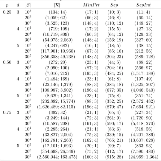
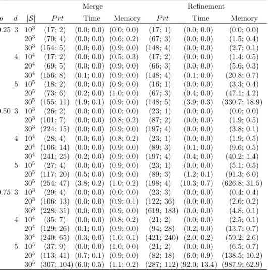
We implemented the proposed partitioning algorithms in C; the code can be obtained from [48]. All experiments are performed on a PC with an Intel Core i7 Quad-Core 3.6 GHz processor with 32 GB of main memory. All times are reported as seconds of CPU time. We monitor the memory allocation of the algorithms with the pidstat command of the sysstat package under Linux and all memory allocation results are reported as Megabytes (MB). We consider two groups of test problems. The first group consists of multi-dimensional reachable state spaces of Markovian models from the literature. The second group consists of a class of randomly generated multi-dimensional reachable state spaces with known minimum Cartesian product partitioning. We use the second group to find out how good the partitioning algorithms perform in terms of number of partitions with respect to the optimal solution.

2.3.1 Test problems from literature

We consider state spaces of call center models with different control policies (N-model, V-model, W-model) [30], a parallel communication software model (courier large, courier medium) [20], a manufacturing systems model with Kan-ban control (kanKan-ban fail, kanKan-ban large) [21], and a queueing model with multiple servers and queues (msmq large) [26]. The V-model has different variations with 2, 3, and 4 types of customers that we consider. ‘V-model (2)’, ‘V-model (3)’ and ‘V-model (4)’ in the results refer to the V-model with 2, 3, and 4 customer types [30].

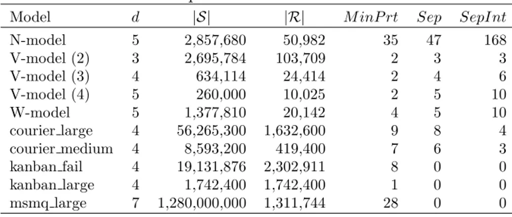
Table 2.1 gives the properties of the first group of test problems. The first four columns give the model name, the dimension of the state space, the size of the product state space, and the size of the reachable state space. The fifth column gives the minimum number of partitions in Cartesian product partitioning. The states of each connected component in the graph, that is obtained by removing the separators from the unit distance graph of R, are in same partition in the

(40)

minimum Cartesian product partitioning of R (see Lemma 5 in [47]). Hence, each partition in the minimum Cartesian product partitioning of R is a union of partitions obtained by removing the separators from the unit distance graph of R. We compute all possible Cartesian product partitionings satisfying this condition in order to obtain the number of partitions in the minimum Cartesian product partitioning. This is trivial when there are small number of separators and intersecting separator pairs. However, the number of Cartesian product partitionings to compute increases exponentially with the number of separators and intersecting separator pairs. We also report two important characteristics of the models. The sixth and seventh columns give the number of separators and the number of intersecting separator pairs, respectively. The reachability of a multi-dimensional state depends on the interaction of the subsystems. Hence, the number of separators and intersecting separator pairs depends on the model and the reachability conditions. There are many different reachability conditions, such as the sum of different subsystem state values might be bounded or a subsystem cannot be in a state depending on other subsystem states. In the N-model, the sum of different subsystem state values is bounded implying more separators and intersecting separator pairs. There is no such interaction in the other models we consider. V-model, W-model, courier large, and courier medium are simpler than the N-model, and have relatively small numbers of separators. There are no separators in kanban fail, kanban large, msmq large, and kanban large, that is, the unit distance graphs of these models do not include any conflicting edges. Therefore, these models can be considered as trivial.

Table 2.1: Properties of models from literature

Model d |S| |R| M inP rt Sep SepInt N-model 5 2,857,680 50,982 35 47 168 V-model (2) 3 2,695,784 103,709 2 3 3 V-model (3) 4 634,114 24,414 2 4 6 V-model (4) 5 260,000 10,025 2 5 10 W-model 5 1,377,810 20,142 4 5 10 courier large 4 56,265,300 1,632,600 9 8 4 courier medium 4 8,593,200 419,400 7 6 3 kanban fail 4 19,131,876 2,302,911 8 0 0 kanban large 4 1,742,400 1,742,400 1 0 0 msmq large 7 1,280,000,000 1,311,744 28 0 0

(41)

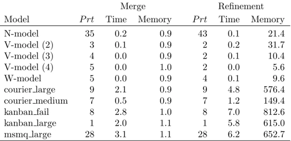
In Table 2.2, we present the results of experiments for the models from lit-erature when the states are processed in lexicographical order. If the states are not given in this order, then it may be easily obtained by sorting. The sec-ond and fifth columns give the number of partitions in the Cartesian product partitionings computed by merge and refinement based partitioning algorithms, respectively. When the states are processed in lexicographical order, both al-gorithms compute the optimal solution for the courier large, courier medium, kanban fail, kanban large, and msmq large models. The merge based algorithm computes the optimal solution of only the N-model among the call center mod-els. The refinement based algorithm computes the optimal solution for all call center models except the relatively complicated N-model. It is reasonable to use merge based algorithm for relatively complicated problems. For all the models, the merge based algorithm requires less time and memory than the refinement based algorithm.

Table 2.2: Experimental results for models from literature when states are pro-cessed in lexicographical order

Merge Refinement Model P rt Time Memory P rt Time Memory N-model 35 0.2 0.9 43 0.1 21.4 V-model (2) 3 0.1 0.9 2 0.2 31.7 V-model (3) 4 0.0 0.9 2 0.1 10.4 V-model (4) 5 0.0 1.0 2 0.0 5.6 W-model 5 0.0 0.9 4 0.1 9.6 courier large 9 2.1 0.9 9 4.8 576.4 courier medium 7 0.5 0.9 7 1.2 149.4 kanban fail 8 2.8 1.0 8 7.0 812.6 kanban large 1 2.0 1.1 1 5.8 615.0 msmq large 28 3.1 1.1 28 6.2 652.7

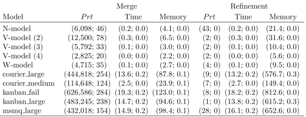
In Table 2.3, we present the results of experiments for the models from liter-ature when the states are processed in random order. For both algorithms, we compute the Cartesian product partitioning by processing the states in 51 ran-dom orderings so as to provide mean values. The second and fifth columns of Table 2.3 give the mean number of partitions together with the confidence inter-val both rounded to the nearest integer for a confidence probability of 95% of the partitionings obtained by merge and refinement based algorithms, respectively. In ‘Time’ and ‘Memory’ columns, the mean values and the confidence intervals for

(42)

a confidence probability of 95% of the experiments are reported. In all columns, the first value in parentheses is the mean and the other value is the confidence interval.

Table 2.3: Experimental results for models from literature when states are pro-cessed in random order

Merge Refinement

Model P rt Time Memory P rt Time Memory N-model (6,098; 46) (0.2; 0.0) (4.1; 0.0) (43; 0) (0.2; 0.0) (21.4; 0.0) V-model (2) (12,500; 78) (0.3; 0.0) (6.5; 0.0) (2; 0) (0.3; 0.0) (31.6; 0.0) V-model (3) (5,792; 33) (0.1; 0.0) (3.0; 0.0) (2; 0) (0.1; 0.0) (10.4; 0.0) V-model (4) (2,825; 20) (0.0; 0.0) (2.2; 0.0) (2; 0) (0.0; 0.0) (5.6; 0.0) W-model (4,715; 35) (0.1; 0.0) (2.7; 0.0) (4; 0) (0.1; 0.0) (9.5; 0.0) courier large (444,818; 254) (13.6; 0.2) (87.8; 0.1) (9; 0) (13.2; 0.2) (576.7; 0.3) courier medium (114,648; 124) (2.5; 0.0) (23.9; 0.1) (7; 0) (2.7; 0.0) (149.4; 0.0) kanban fail (626,586; 284) (19.3; 0.2) (123.0; 0.1) (8; 0) (18.2; 0.2) (812.6; 0.0) kanban large (483,245; 238) (14.7; 0.2) (94.6; 0.1) (1; 0) (13.8; 0.2) (615.2; 0.3) msmq large (432,018; 154) (14.9; 0.2) (98.4; 0.1) (28; 0) (16.1; 0.2) (652.6; 0.0)

The partitioning size and the memory requirement remain the same for the refinement based algorithm, but the time requirement increases when the states are processed in random order. In all of the models, the number of separators is small, so the increase in time is not due to the refinement of the graph and updating of separators, but due to the graph construction. These results suggest that cache is more efficiently used while accessing the states when the states are ordered lexicographically since each state becomes a child of the last accessed state in the AVL tree. Hence, insertion to the tree becomes much more efficient for the lexicographic ordering of the states. The order of states is much more important for the merge based algorithm. In this algorithm, two partitions are merged along dimension h if the subsets of their subsystems are the same in all dimensions except h. When the states are ordered lexicographically, a partition is merged with all possible partitions along a dimension before it is merged with a partition in another dimension. When the states are ordered randomly, parti-tions are merged along random dimensions depending on the order of the states. Hence, all possible partitions along a dimension are not considered. Therefore, the number of partitions for random ordering of the states increases by a factor between 174 (N-model) and 483,000 (kanban large) on average with respect to