424 IEEE TRANSACTIONS ON PARERK
10
5
‘0 5 10 15 U) 25 30 35 40 4 5 k 5 0
Fig. 2.
space by Patrick-Fisher’s algorithm (solid line) and E (dotted line). Bayes error estimates for SONAR data transformed to IO-dimensional
high-dimensional data these results might be more in favor of E.)
This is a result of the fact that each iteration of simplex requires that the samples be transformed to the low-dimensional space, and then the Bayes error estimated in that space, which in turn requires computation of distances, determination of optimal thresholds, and classification. The iterative process is repeated until the convergence is achieved. In contrast,
FLD
and KL are noniterative techniques, which merely compute eigenvalues and eigenvectors of certain ma- trices. For PF, which is also an iterative algorithm, the difference inCPU timing is about an order of magnitude for SONAR data.
V. SUMMARY
The aim of this correspondence was to investigate the possibility of constructing such linear transformation of labeled multidimensional vectors that would hopefully ensure the maximum attainable classifi- cation accuracy in the transformed space. In other words, the goal was to come as close as possible to computing a transformation matrix that would minimize the Bayes error in the low-dimensional space, and to devise a practical algorithm for such purpose. The proposed algorithm, called E, consists in finding such matrix that minimizes the estimate of the Bayes error, computed on the training data set projected to the low-dimensional space. The most reliable technique for Bayes error estimation available was used, and the simplex algorithm played the role of the optimization algorithm.
In all examples, E demonstrated superior performance in compar- ison with standard algorithms, coming close to the theoretical limits
on classification accuracy. This is payed through significant increase of the computational load. Still we managed to keep its complexity within realistic bounds, thus realizing designated goals.
ACKNOWLEDGMENT
The author thanks M. MilosavljeviC for continuous support and M.
MarkoviC for helpful discussions and for suggesting formula (4). REFERENCES
[ I ] J. A. Nelder and R. Mead, “A simplex method for function minimiza- tion,” Comput. J., vol. 8, pp. 308-313, 1965.
[2] L. F. Guseman, Jr., B. C. Peters, Jr., and H. F. Walker, “On minimizing the probability of misclassification for linear feature selection,” Annals Statist., vol. 3, pp. 6 6 1 4 6 8 , 1975.
ANALYSIS AND MACHINE INTELLIGENCE. VOL. 16, NO. 4, APRIL 1994
S . A. Dudani, K. J. Breeding, and R. B. McGhee, “Aircraft identification by moment invariants,” IEEE Trans. Comput., vol. C-26, pp. 39-45, 1977.
A. K. Jain and W. G. Waller, “On the optimal number of features in the classification of multivariate Gaussian data,” Pattern Recogn., vol. IO, pp. 365-374. 1978.
S. J. Raudys, “Determination of optimal dimensionality in statistical pattern classification,” Pattern Recogn., vol. 11, pp. 263-270, 1979. G. Biswas, A. K. Jain, and R. C. Dubes, “Evaluation of projection algorithms,” IEEE Trans. Pattern Anal. Machine Intell., vol. PAMI-3, P. A. Devijver and J. Kittler, Pattern Recognition: A Statistical Ap- proach.
J. Kittler, “Feature selection and extraction,” in Handbook of Pattern Recognition and Image Processing, T. Y. Young and K.-S. Fu, Eds. Orlando, FL: Academic, 1986.
K. Fukunaga and D. M. Hummels, “Bayes error estimation using Parzen and I;-” procedures,” IEEE Trans. Pattern Anal. Machine Intell., vol. PAMI-9, pp. 634-643, 1987.
R. P. Gorman and T. J. Sejnowski, “Analysis of hidden units in a layered network trained to classify sonar targets,” Neural Networks, vol. I, pp. 75-89, 1988.
K. Fukunaga, Introduction to Statistical Pattern Recognition, 2nd ed. Boston: Academic, 1990.
P. PejnoviC, “Application of moment invariants in visual pattern recogni- tion” (in Serbo-Croatian), M.S. thesis, Faculty of Electrical Engineering, Univ. of Belgrade, Belgrade, Yugoslavia, 1991.
Lj. ButuroviC and Z. StojiljkoviC, “PARIS-pattern analysis and recog- nition interactive system,” Pattern Recogn., vol. 24, p. 11, 1991. Lj. J. ButuroviC, “On the minimal dimension of sufficient statistics,” IEEE Trans. Inform. Theory, vol. 38, pp. 182-186, 1992.
pp. 701-708, 1981.
Englewood Cliffs, NI: prentice-Hall International, 1982.
On a Parameter Estimation Method
For Gibbs-Markov Random Fields
Mehmet I. Giirelli and Levent OnuralAbstract-This correspondence is about a Gibbs-Markov random field (GMRF) parameter estimation technique proposed by Derin and Elliott. We will refer to this technique as the histogramming (H) method. First, the relation of the H method to the (conditional) maximum likelihood (ML) method is considered. Second, a bias-reduction based modification of the H method is proposed to improve its performance, especially in the case of small amounts of image data.
Index Terms-Image modeling, texture, Gibbs-Markov random fields, parameter estimation, pattern recognition.
I. INTRODUCTION
Texture plays a very important role in image processing. In the lit- erature, there exist several techniques for the analysis and processing of textured images, such as classification and identification [l], and segmentation and restoration [2]-[9]. Among the most well-known texture models are the autoregressive models [ 2 ] , random mosaic models [lo], and stochastic models [3]-[9], [ l I]-[14]. The Gibbs Manuscript received March 11, 1991; revised June 1, 1993. This work was supported in part by the Scientific and Technical Research Foundation of Turkey (TUBITAK) under the COST21 1 project grant. Recommended for acceptance by Associate Editor A. Blake.
M. I. Giirelli was with the Department of Electrical and Electronics Engineering, Bilkent University, 06533 Ankara, Turkey. He is now with the Signal and Image Processing Institute, Department of Electrical Engineer- i n g S y s t e m s , University of Southem California, Los Angeles, CA 90089.
L. Onural is with the Department of Electrical and Electronics Engineering, Bilkent University, 06533 Ankara, Turkey.
IEEE Log Number 9214458.
IEEE TRANSACTIONS ON PATTERN ANALYSIS AND MACHINE INTELLIGENCE, VOL. 16, NO. 4, APRIL 1994
U
w’
425t
v
w
s
u0
v0 t’
and Markov random fields are among the most powerful stochasticmodels [ 1 I]-[ 141. In this correspondence, we will collectively refer to both models as the Gibbs-Markov random field (GMRF) model. Several segmentation and restoration algorithms based on the GMRF model can be found in [4]-[9].
In many applications of the GMRF texture model, it is usually necessary to estimate the model parameters (see, for example, [7]).
The coding and pseudo-likelihood methods are among the most widely known parameter estimators [12], [13]. The pseudo-likelihood method is an extension of the coding method from a single coding to the whole image region, disregarding the lack of conditional independence among the pixel values. In this correspondence, the coding and pseudo-likelihood methods will be collectively referred to as the maximum likelihood (ML) method. Another method, which we will call as the histogramming (H) method, has been proposed by Derin and Elliott [7].
In this correspondence, we concentrated on the H method. Our aim is twofold. First, we want to clarify the properties of the H method and establish its relation to the well-known ML method. Second, we propose a modification to the H method to improve its performance for binary GMRF’s, especially in the case of small amounts of image data. In the case of small amounts of image data, the H method suffers from two facts. First, the bias in parameter estimates becomes more emphasized, and second, in the H method, some data is generally discarded, which usually results in an insufficient amount of data to obtain the GMRF parameter estimates uniquely. As will be clarified in the forthcoming sections, the modification we proposed in this paper addresses these two problems simultaneously.
In Section I1 mathematical preliminaries are given. In Section 111, the H method is derived. Section IV is aimed at clarifying the link of the H method to the ML method. In Section V, the bias in the
H method is described. In Section VI, a method to reduce the bias is proposed. In Section VII, we give some experimental results, and, finally, some conclusions are given in Section VIII.
11. MATHEMATICAL PRELIMINARIES
We model the image region as a set of rectangularly placed pixels denoted by ‘P. We will refer to the numerical realization of the random field at pixel i E 2, by the notation y ( i ) . For the numerical realization over a subset
R
C
D , the notationy ( R )
will be used. Detailed descriptions of GMRF’s and related concepts such as neighborhood systems and codings can be found in [7] and [11]-[13]. The shape of the neighborhood of an interior point i of27
will be assumed to be independent of its location in 2, and will be denoted by ?lt (or simply1 1 ) . For a given coding
C,
GMRF’s have the following (conditional)independence property [ I I]:
P(Y(C)13.’(P\C)) =
~ P ( . ? / ( ~ ) I Y ( v , ) ) .
(1),E<’
This property is very important in the formulation of the H and ML methods. To keep the discussions clear, we will refer to a binary GMRF described by the conditional probability distribution [ 111.
J 7’ P ( y ( i ) =
.sIy(i/,))
= ~1 + e T ( 2 )
and S . ( 1 . U ’ . r . (1’. t . t ’ . ir. w ’ E (0.1) are the pixel values whose
relative locations are as shown in Fig. I . The vector of model parameters A = [ (I j j , .j,. j,,, ,j(
1’
will be called the GMRF parameter vector. Multilevel GMRF’s of the above parametric form may be found in [7] and [ 111.Fig. 1. Neighborhood pixel values
111. DERIVATION OF THE HISTOGRAMMING (H) METHOD
The GMRF parameter estimation method described in this section has been proposed by Derin and Elliott [7]. We will refer to this method as the histogramming (H) method. We start by partitioning the set of possible neighborhood realizations into I< groups such that within the kth group ( k = 1.. . . ,
I<)
each neighborhood realization yields the same coefficient vector Q, given as(4) A possible grouping is to assume that each neighborhood realization is a distinct group. We will indicate the correspondence of any variable to the kth group by the subscript k . For every neighborhood realization y k ( i l ) belonging to the kth group, we have a fixed (conditional) probability for the pixel value to be 0 or 1 for a given set o f p a r a m e t e r s . L e t p t = P ( s = l l ~ t ( ~ ~ ) ) a n d q t = 1 - p t = P ( s =
O I Y k ( ? ) ) ) . Then, using (2) and ( 3 ) , we have Tk = l n ( p k / q k ) , where TA = .rzg. Hence, we obtain a system of I< linear (and consistent) equations in terms of the GMRF parameters as
st
= [l ( U+
U,’) ( U+
( 9 ‘ ) ( t+
t’) (U‘+
W ‘ f .n
+
( U+
U ’ ) J , <+
( 1 ’+
v ’ ) * A .+
( t+
f’)d,,,+ ( u > + u * ’ ) , j , . = d k A - = I , . . .
.S.
(51
where d l = hl(PI,/(Ik).
To estimate g, the d k ’ s in (5) will be estimated first. This is done through histogramming, as follows. Suppose that there are a total of
L k pixels in a given coding C of 2, with neighborhood realizations
from the kth group. From (l), the pixel values corresponding to these
L t locations become statistically independent when conditioned on the numerical realization of the set 27
\
C.
Let Y j , k be the numberof 1 outcomes in these Lk observations. It is assumed that
Y(73
\
C )is given; hence Lk is deterministic and -\-~.k is the outcome of a random quantity. Then, an estimate of d k in (5) can be given as
To justify this estimate, note that for large L k , we have the asympthotic behavior
(7) Using (5) and (6), to estimate g we may try to solve the system of equations given as
Pk L t - -TI k (Ik
+ -.
~h-1 , A
which may be put into matrix form as
s,
g =n
(9) with and c i k being the corresponding rows ofS,
andi,
re- spectively. In general, it is not necessary to include the equations corresponding to every possible neighborhood realization to the system of equations in (9). The system in (9) will usually contain less than I< equations. This is because for A = 0 or )VI 1 = L A ,426 IEEE TRANSACTIONS ON PATTERN ANALYSIS AND MACHINE INTELLIGENCE, VOL. 16, NO. 4, APRIL 1994
(6) and (8) will be undefined and the corresponding image data will be discarded. This is one of the main weaknesses of the H method, as will be discussed in forthcoming sections. Furthermore, for some group of neighborhood realizations, Lk may be zero. Using (9), an estimate
ZH
of the parameter vector may be obtained as&,
= X;’iwhere
X:
is the pseudoinverse of the matrix Xr.. If Xr is a full (column) rank matrix, thenX
:
= ( X ~ X , ) - ’ - X ~ . IfX,.
is not full rank, the resulting parameter estimates are generally highly corrupted. For certain multilevel GMRF’s, the above formulation can be simply modified by considering every pair of pixel values with a given neighborhood realization [7]. Also, the histogramming may, in practice, be done over the whole image instead of a single coding.Iv.
RELATION OF THE H METHOD TO THE ML METHOD The coding form of the ML estimate maximizes the probabil- ityP(Y(ClY(D
\
C ) ) )
or, equaivalently, the log-likelihoodfunction(LLF) [Ill-[I31
L ( C ) = C l n ( P ( y ( i ) I Y ( v z ) ) ) (10) 1 E C
as a function of g. The terms in (IO) can be grouped under Ii terms, each of which corresponds to one of the
I<
groups of neighborhood realizations as described in Section 111. So we haveh’
L ( C )
= . C k ( C ) , ( 1 1 ) k = l where L k ( C ) = N 1 . k I.(P(Y(i) = l l Y k ( 1 7 ) ) ) + ( L k - N l , k ) l n ( P ( y ( i ) = O I Y k ( 1 7 ) ) ) . (12) Although the discussion can be easily extended to multilevel GMRF’s described in [7], we will consider the binary model given by (2) and (3), for which we havewhere T k =
J - Z ~ .
The gradient of&(e)
denoted asv&(C)
isgiven by
and V C L k ( C ) , the second derivative matrix of L k ( C ) , is given by
The value of -/k is strictly positive for any L k
>
0 ; hence VOCk(C)is negative semidefinite, with one negative eigenvalue --/k corre- sponding to the eigenvector
sk,
and the remaining eigenvalues are zero. So&(e)
is a convex cap function of the parameter vector - J. From (13), it is easy to see that,&(e)
has constant values on(n? - 1 )-dimensional hyperplanes in the parameter space where m is the dimension of the parameter vector, g (n? = 5 for the model ( 2 ) , (3)). From (1 I), we also deduce that the LLF is a convex cap function. From (l4), it is clear that L k ( C ) will have a maximum value only if lv1,h
#
0 and :bTl,k#
L k . In any case, &(C) is upper bounded. In Fig. 2, a typical & ( C ) is plotted as a function of ;?h andIf there exists a set of ni groups of neighborhood realizations for which . k
#
0 and :y1 .k#
L k , and if the corresponding coefficient vectors J - ~ are linearly independent, then the LLF will have a unique maximum (for which has a finite Euclidean norm). This fact is easily verified by noting from ( I I ) , (15) that, under the above conditions, the second derivative matrix of LLF will .be negative definite (hence LLF will be strictly convex cap), and also the value of LLF will be decreasing in any direction in the parameter space asFig. 2.
and assuming N 1 . k
#
0 and N 1 . k#
L k .A typical l k (C) surface as a function of /318 and d,. (&,, = d, = 0 )
the norm of g goes to infinity. However, the LLF may have a unique maximum point under much weaker conditions.
Using (5) and (14), it is easy to show that if the asymptotic behavior in (7) holds, then the hyperplanes over which &(C)’s achieve their maxima will intersect at the point corresponding to the parameter vector of the GMRF under consideration. At this point, the LLF will achieve its global maximum. This suggests that an interesting approach to estimating -J may be to search for an intersection for these hyperplanes. For a given & ( C ) for which N 1 , k
#
0, L k . the hyperplane equation can be obtained by equating the gradient in (14) to zero, which yields the linear equation in gNote that the resulting system of linear equations is exactly the same as the system given by (8), and it may be solved by a least squares method. Hence we obtained the H method. In summary, ML method maximizes the LLF whereas H method tries to achieve this through maximizing individual terms Lk (C). This relationship of H and ML methods will still. hold if the quantities
Avl
. k and Lk are determined from the whole image region instead of a single coding.Since the ML method requires optimization techniques, the H method seems computationally more feasible than the ML method, es- pecially for applications involving parameter estimation over several subregions of a given image. On the other hand, since the H method discards the data corresponding to the case . k = 0 , and N1 , h = Lk,
the parameter estimates may be highly corrupted especially in the case of parameter estimation over small subregions of a given image.
V. BIAS IN H METHOD
Any bias in the vector in (9) is reflected in the
GH
vector through the transformation.&
=S , f d .
In this section, we will formulate the bias for a given entry n^k of2
vector for binary GMRF’s. Since the analysis in this and the next section is done for an arbitrary but fixed group of neighborhood realizations, we will drop the subscript k, which refers to the kth group of neighborhood realizations. For a givenL
and p , and employing the independence property ( l ) , .Vl can be shown to have binomial distributionIEEE TRANSACTIONS ON PATTERN ANALYSlS AND MACHlNE INTELLIGENCE. VOL. 16, NO. 4, APRIL 1994 421
L =
12 L = 2 0L
= 50 s1
3 - 1-
-2-
0.2 0.4 0.6 0.8 1 P -31 Fig. 3.However, in the H method, we omit the cases where N I = 0 or L. So the distribution is
Curves of bias
B(L,p)
ina^
for various values of L .mIL(N1IL) = P(N1lLV1
#
0 and NI#
L )Therefore, the expected value of
d^
is given by(19)
where E{.} is the statistical expectation operator and the notation d =
fi(
L , NI ) is introduced to emphasize the dependence of d on L and N I . For any given L and p , the bias, B( L , p ) , in d is given byB ( L , ~ ) = € ( L , p )
-
d where d = In (1 -",>.
(20) In Fig. 3, bias curves are plotted as a function of p and for several values of L. From the curves, it is seen that for large L the bias is smaller.VI. REDUCTION OF BIAS IN THE H METHOD
As emphasized by the notation (i = f i ( L ,
NI),
(i is a function of L'and N I , which may be interpreted as a look-up table indexed by L and N I = 1,.. .
, ( L - 1 ). In this section, we will consider another estimate d' of d as a function of L and J ~ I , i.e.,d' = D * ( L , N I ) N1 = O ; . . , L . (21) The problem may be interpreted as the design of a new look-up table D * ( L , N I ) . The design criteria will be bias reduction, and we will include cases NI = 0 and N I = L. The bias L?*(L,p) in d* is given by B * ( L , p ) = € * ( L , p ) - d, where
L
E * ( L . p ) = D ' ( L . N I ) f , . , , L ( - ~ l I L )
N 1 = O
is the expected value of D * ( L , L V I ). Note that for given L , € * ( L , p ) is a polynomial in p of order L . On the other hand, the variable d
given in (20) can be represented only by an infinite order polynomial. Therefore, B * ( L , p ) can not be made identically zero for all p E
( 0 . 1 ) . So, instead of removing bias, we may try to choose D* ( L , A'17~ )
TABLE I
LOOK-UP TABLE EXAMPLES FOR L = 5
so as to approximate d by E * ( L . p ) as a function of p for a given L . Therefore the problem reduces to approximating the variable d with a finite order polynomial. To accomplish this, we may force the bias to be zero for a finite number of values for p , i.e., B * ( L , p , ) =
0 j = 0, ., J where p , E ( 0 , l ) are some chosen values for y . Hence, we obtain linear equations in terms of the to be determined variables D * ( L . N 1 ) , N 1 =
O , . . . , L
as(23) The above system of linear equations may be solved by a linear least squares method. After solving for the unknown D* ( L . -VI ) variables, one may put the results as a look-up table, and for any given L and
Ail one may use
D *
( L , lV1 ) as an estimate of d . For the estimation of g, the system of equations in (8) may be rewritten as-
r f g = d; where d; = D * ( L L , X I , k ) . (24) The choice of p, 's in (53) determines the bias and mean-squared- error properties of the estimator. Since it is desirable to have
D * ( L , N 1 ) = - D * ( L , L - X I ) n = O , . . . . L , the p , ' s must be chosen symmetrically around p = 0.5. In Table I, a sample look-up table for L = 5 is given both for the H method (i.e., D ( L , XI ) ) and for the modification proposed in this section (i.e., D* ( L , :VI )). To compute
D*
( L , Arl ), we have usedp , E { p I p = 0 . 5 + ( 0 . 0 5 + 0 . 0 1 k ) k=0:..,15}.
In Fig. 4, curves of d , & ( L , p ) , and € * ( L , p ) are plotted as a function of p for L = 5 (the look-up table in Table I is used). Note that the bias corresponds to the vertical difference between the d- curve and the E ( L . y ) or E * ( L , p ) curves. At this point, it must be emphasized that in general the matrix S, in (9) will be different in the H method and its modification proposed here (since we include the equations corresponding to SI = 0, L k ) . Therefore, the effects of bias in d and d' on the estimate of -J will not be directly comparable,
as in Fig. 4.
The mean squared errors (mse's) in
(f
and d* are given by M ( L , p ) = E ( ( 2 - d ) ' } , W * ( L , y ) = E { ( d * - d ) ' } , ( 2 5 ) respectively. Both expectations are with respect to N I . Note that in M ( L , p ) , the distribution is given by (18), and for M * ( L , p ! the distribution is given by (17). In Fig. 5, mse curves of d* and d are plotted as a function of p for L = 5 (the look-up table in Table I is used). Again, it must be noted that the effects of the mse in dand d* on the estimation of -.' will not be directly comparable from Fig. 5, because the
S,
matrixes for the H method and its modification proposed here will be in general different.In this section, we basically proposed a modification to the H method by using the bias reduction criterion. In this alternative method, we included the case of SI = 0 and *VI = L to the estimation process. Therefore, we have attacked two disadvantages of the H method simultaneously, namely the bias and the case of
428 IEEE TRANSACTIONS ON PATTERN ANALYSIS AND MACHINE INTELLIGENCE, VOL. 16, NO. 4, APRIL 1994
Fig. 4. Curves of d . & ( L . p ) , and & * ( L , p ) for L = 5 .
I . I I I 1 1 . I I I I I ' I I I
!
II
I 0.2 0.4 0.6 0.0 1 P Fig. 5. Mse curves of d* and (i for L = 5.Estimation of parameters over small subregions of a given image is usually required in many problems such as texture segmentation. In such circumstances, due to the limited amount of image data, it is very likely that the case of N I = 0 or N I = L will be met. Since in the H
method the corresponding data is discarded and no linear equation is obtained for the corresponding classes of neighborhood realizations, the system of linear equations in (9) usually contains a highly limited number of equations to give good parameter estimates. It is even very likely that the matrix
S,
may not have full column rank, in which case the linear least-squares solution will not be unique (the transformationGH
=-Y:d
will give the minimum norm solution). This may result in highly corrupted parameter estimates. The number of rows ofS,
may significantly increase by the inclusion of A71 = 0and N I =
L
into the parameter estimation. For the above reasons, we included the case of ~ Y I = 0 andIVI
= L in our look-up table design. Hence, it is more likely to have a full column rankS,
matrix.
Although this new estimator for d may introduce a larger mse for a range of y values, the combined effect of the increased number of rows in
S,
and the averaging effect of the transformationSti
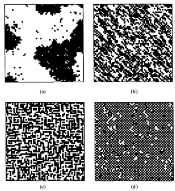
can be expected to reduce the extra mse on the parameter estimates. Therefore, the bias reduction approach proposed here seems to be a very reasonable criterion for the look-up table design. Also note that once the look-up tables are prepared, the computational complexities of the H-method and its modification will be almost the same.Fig. 6. a = 0,
Sample GMRF textures with parameters: (a) a = -4, ;3& = fit,
= beta, = 1 , &,, = d, = -1. (d) a = 0, d h = d, = -1, = P v r L = d,. = 1. (b) a = -1.5. j?h =dtr = 0, dm = 1.5, /?r = 0. (c)
= = 1.
TABLE I1
PARAMETER FSTIMATION RESULTS
VII. EXPERIMENTAL RESULTS
In this section, we will present experimental results corresponding to four different sets of specified parameters and various image region sizes. The test images have been synthetically generated by the Gibbs sampler algorithm using the model in (2) and (3) [ 5 ] . Typical sample textures are shown in Fig. 6 for each parameter set.
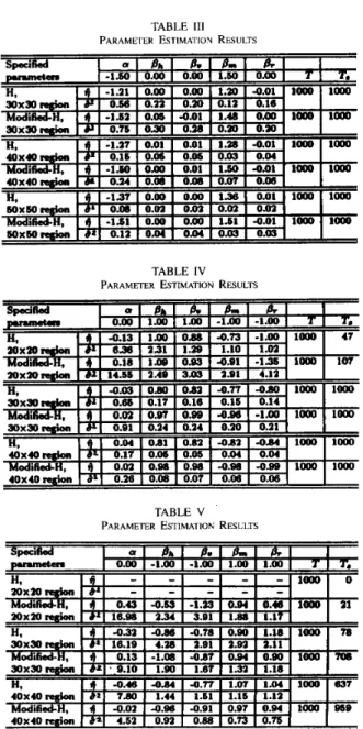
Experimental results are summarized in Tables 11-V. The first col- umn of each table indicates the method of parameter estimation and size of the image region (only one of the four codings corresponding to a second-order neighborhood structure has been used [ 1 11). Tables
11-V include the results for both the H method described in Section
I11 and its modification (referred to as
modified-H on the tables) based on the bias reduction criterion described in Section VI. The columns labeled asT
indicate the number of times the corresponding experiment has been performed and T, is the number of successful trials. By a successful trial we mean a performance of the experiment in which the matrixS,.
comes out to be full rank (so that the least- squares solution of the resulting linear equations will be unique).IEEE TRANSACTIONS ON PATTERN ANALYSIS AND MACHINE INTELLIGENCE, VOL. 16. NO. 4, APRIL 1994 429
TABLE III
PARAMETER ESTIMATION RESULTS
TABLE IV
PARAMETER ESTIMATION RESULTS
TABLE V
PARAMETER ESTIMATION RESULTS
I
8.1 A1a1
Note that in the modified-H method, the success rate is always at least as large as the success rate of the H method. This is because the modified-H method uses the data for which
SI
= 0 or L for a set of L values, as will be described in this section. The sample means6
and variances 5’ of each parameter is computed over the successful trials only. More specifically,
where
<,
denotes the value of a parameter<
E {rt. j),. ,j, . , I , ! , . ( I , }for the ith successful trial.
For both the H and modified-H methods, we have discarded the data corresponding to L
<
5. In the modified-H method, look-up tables based on the bias reduction criterion have been generated only for L = .j.G:...
11. For L>
11, the estimator of d given in (6) is used for both methods. This is because an important portion of the discarded data in the H method usually corresponds toL = 5 , 6 , .
.
. , 11 for small image region sizes. Furthermore, the bias is not very significant for L>
11.For generating the look-up tables, the p, values in (23) have been taken as
pJ E { p
I
p = 0.5+(0.05+
0.01k) k = 0.. ..
.15]for
L
= 5 , 6 ; . . , 1 0 ,a d pJ E { p
I
p = 0.5+0.01k k = 0... .
, 2 5 }for L = 11.
Although no specific strategy has been followed in choosing the pJ values as given above, we have obtained good results in many experiments for small image region sizes.
The results summarized in Tables 11-V indicate that the modified- H method usually yields a lower bias and also that the success rate is higher than the H method. The sample variances indicate that, for many applications, the H and modified-H methods have a reasonable variance. It must be noted at this point that once the look-up tables are prepared, the computational complexity of the method proposed in this correspondence and the H method are almost the same.
VIII. CONCLUSION
An advantage of the H method over the ML method is in its computational simplicity. The ML method requires the maximization of a log-likelihood function, whereas the H method involves simple histogramming, a look-up table operation, and computation of the pseudoinverse of a matrix with generally reasonable dimensions.
For its computational simplicity, the H method is well suited to problems involving parameter estimation over several subregions of a given image. On the other hand, the omission of data (for
XI , L = 0.
Ln-)
in the H method may result in very poor performance over small image regions. Even more, theS,.
matrix may not have full columirank. However, in problems such as image segmentation it is usually required to estimate the GMRF parameters over several small subregions of the given image. Therefore it is very important to have an estimator that is both computationally simple and capable of yielding sufficiently good parameter estimates even in the case ofa small amount of image data.
In this correspondence, we proposed a modification to the H method to improve its performance, especially in the case of a small number of observations while preserving its computational advantage over the ML method. This modification is computationally almost as easy as the H method. Furthermore, it does not suffer from the data omission and hence it is more likely that S,. matrix will have full column rank. The extension of the method to multilevel GMRF’s and the methodology for choosing pJ values in (23) may be topics of future research.
ACKNOWLEDGMENT
The authors thank Dr. E. Arikan for his valuable discussions. RE FER EN
c
Es
[ I ] R. L. Kashyap and A. Khotanzad, “A model-based method for rotation invariant texture classification,” IEEE Trans. Pattern Anal. Machine
Infell., vol. PAMI-8, no. 4. pp. 4 7 2 4 8 1 , July 1986.
121 K. Deguchi and I. Morishita, “Texture characterization and texture-based image partitioning using two-dimensional linear estimation techniques,”
IEEE Trans. Comput.. vol. C-27, no. 8, pp. 739-745, Aug. 1978. [3] R. Chellappa and R. L. Kashyap, “Digital image restoration using spatial
interaction models,” lEEE Trans. Acoust., Speech. Signal Processing,
vol. ASSP-30, no. 3, pp. 4 6 1 4 7 2 , June 1982.
141 F. R. Hansen and H. Elliott, “Image segmentation using simple Markov field models,” Comput. Graphics Image Processing. vol. 20, pp. 101-132, 1982.
430 IEEE TRANSACTIONS ON PATTERN ANALYSIS AND MACHINE INTELLIGENCE, VOL. 16, NO. 4, APRIL 1994
[5] S. Geman and D. Geman. “Stochastic relaxation, Gibbs distributions, and the Bayesian restoration of images,” IEEE Trans. Pattern Anal. Machine Intell., vol. PAMI-6, no. 6, pp. 721-741, Nov. 1984. [6) H. Derin and W. S. Cole, “Segmentation of textured images using Gibbs
random fields,” Comput. Vlsion, Graphics, Image Processing, vol. 35, pp. 72-98, 1986.
[7] H. Derin and H. Elliott, “Modeling and segmentation of noisy and textured images using Gibbs random fields,” IEEE Trans. Pattern Anal. Machine Intell., vol. 9, no. I , pp. 39-55, Jan. 1987.
[8] C. S. Won and H. Derin, “Unsupervised segmentation of noisy and textured images using Markov random fields,” CVGIP: Graphical Models and Image Processing, vol. 54, no. 4, pp. 308-328, July 1992. [9] F. S. Cohen and Z. Fan, “Maximum likelihood unsupervised textured image segmentation,” CVGIP: Graphical Models and Image Processing, vol. 54, no. 3, pp. 289-251, May 1992.
[IO] N. Ahuja and A. Rosenfeld, “Mosaic models for textures,” IEEE Trans. Pattern Anal. Machine Intell., vol. PAMI-3, no. 1, pp. 1-1 1 , Jan. 1981. [ 11) G. R. Cross and A. K. Jain, “Markov random field texture models,”IEEE Trans. Pattern Anal. Machine Intell., vol. PAMI-5, no. 1, pp. 25-39, Jan. 1983.
[12) J. Besag, “Spatial interaction and the statistical analysis of lattice systems,’’ J. Roy. Statist. Soc., Series E . vol. 36, pp. 192-236, 1974. [I31 -, “On the statistical analysis of dirty pictures,” J. Roy. Statist. Soc.,
Series E , vol. 48, pp. 259-302, 1986.
[ 141 C. 0. Acuna, “Texture modeling using Gibbs distributions,” CVGIP: Graphical Models and Image Processing. vol. 54, no. 3, pp. 21G222, May 1992.
Contribution to the Determination of Vanishing Points
Using Hough Transform
Evelyne Lutton, Henri M a h e , and Jaime Lopez-Krahe
Abstract-We propose a method to locate three vanishing points on an image, corresponding to three orthogonal directions of the scene. This method is based on two cascaded Hough transforms. We show that, even in the case of synthetic images of high quality, a naive approach may fail, essentially because of the errors due to the limitation of the image size. We take into account these errors as well as errors due to detection inaccuracy of the image segments, and provide a method efficient, even in the case of real complex scenes.
Index Tenns-Bias and errors of the Hough transform, Hough trans- form, orthogonal directions detection, vanishing points detection.
I. INTRODUCTION
In many tasks of artificial vision, an accurate location of vanishing points is a first step toward three-dimensional (3D) interpretation. Vanishing points are defined in the,image plane as those points where the images of all 3D scene lines, parallel to some space direction, converge. To one 3D space direction is attached one vanishing point on the image plane and conversely.
Detection of vanishing points, which is of little help in natural outdoor scenes, becomes of prime importance in the man-made environment where regular block looking structures or parallel align- ments (streets, pavements, railroad) abound. We have the Italian Quattrocento to thank for the deep comprehension of the formation Manuscript received October 9, 1990; revised September 17, 1992. This The authors are with Departement Images, Telecom Paris, Cedex, France. IEEE Log Number 9206561.
work was supported by DRET and in collaboration with MATRA.
F
q g . 1. A I , 1 2 , and 1 3 are lines of the 3D space parallel to the direction
I T . 61. h:,. and 6s their images on the-image plane. E 1 % E:, , and 63 converge to the vanishing point associated to I ; .
of perspective images,’ a comprehension that has been a constant preoccupation of the theoricians in aesthetics up to the 20th century.’ Traces of rigorous mathematical bases are found mainly at the comer of the 18th-19th centuries.” Although the geometrical construction of vanishing points may become very complex when no hypothesis is made on the vision system, in the case of a perfect conic projection (pinhole cameras) it may be solved easily, since the image of a straight line remains a straight line. We will stay in the assumption of conic projection throughout this paper.
Most of the existing methods to detect automatically these vanish- ing points stand on the use of the Hough transform, explicitly or not
[16], [20], [21]. Hough transform is a global technique for detecting parametrical structures in images [ 5 ] , [7], [17]. Some primitives are detected in the image, and then mapped into a parameter space; underlying structures are detected by searching for clusters in this parameter space. Two methods can be distinguished to fill the accumulators of Hough space [ 171.
The “one-to-many’’ (I-to-ru ) transform, used most of the time, where for each feature point in the picture plane, several accumulator cells are incremented.
The “many-to-one’’ (rn-to-I), where we make use of several feature points in the image plane to increment exactly one accumulator cell.
For the application of vanishing points detection, the primitives are line segments. The vanishing points are thus characterized as those points where most of the supporting lines of these segments intersect (Fig. 1). Most of the time, these points are located far away from the image limits and even can be at infinity (for frontal lines).
So, the most important problem of the detection of vanishing points with the help of the Hough transform’is the choice of the Hough space parameterization. Two main orientations have appeared in the literature, following the I-to- m or the nt-to-1 transforms; they are chronologically:
The I-to-nr approach with:
Kender [9] in 1979 who uses, directly on the image plane, circles passing through the origin, and proposes either a search in a tridimensional space or two successive transforms;
Ballard and Brown [2] in 1982, who propose a ( k / r , H ) pa- rameterization, with k constant, for the image primitives, which permits restriction of parameter space;
‘L. B. Alberti, “De pictura” (manuscript 1435), printed in Bas1 (Swiss), ’E. Panovsky. “Die Perspektive als symbolische Form,” Berlin. 1927. 3 G . Monge, “GCometrie descriptive.” Leqons donnkes aux Ecoles Normales 4J. V. Poncelet, “Trak2 des propriCtCs projectives des figures,” Paris, 1822. 1540.
de l’an Ill de la R@uhlique, Paris. 1798.