OPTIMAL COKTÄOL
FO SlllYE
И Я ь±
SYSTEMS
А
T H E S I S
TO TMEDEPAIlTMEr-lT OE ELECTSa
CAİ AWL
ELECTSONÍCS ШЧОШЕЕШГчО
THE INSTITUTS OF ENGINBEMIMO AWL SCiST^OES
O F B Í L k B K X U ÎH Y B 2 S İ T Y
2Г!
FULFÍLLMSNT OF T B E ^Q U ÎSEM EN TS
r'İJfJİ'c. Û kıİiLİhA ixáASXSH OF SCIENCE
Ο ί Λ ί έ Χ ’l ) N ¿ ijuly,
1 9 9 Ί
TJ
Z 1 L O ■ U S 3 / э з ?INVERSE OPTIMAL CONTROL AND POSITIVE
REAL SYSTEMS
A T H E SIS S U B M IT T E D T O T H E D E P A R T M E N T O F E L E C T R IC A L AND E L E C T R O N IC S E N G IN E E R IN G AND T H E IN S T IT U T E O F E N G IN E E R IN G AND SC IE N C E S O F B IL K E N T U N IV E R S IT Y IN P A R T IA L F U L F IL L M E N T O F T H E R E Q U IR E M E N T S F O R T H E D E G R E E O F M A S T E R O F S C IE N C E ^•İMaa. lio o l.By
^
^
~
Yılmaz ÜNAL
July 1997
TJ
2Sîo
•Ü53
I certiiy that I have read this thesis and that in my opinion it is fully adeciuate, in scope cind in cjuality, as a thesis for the degree of Master of Science.
r
_________ ______________________________
Prof. Dr. A. Bülent ÖZGÜLER (Supervisor)
I certify that I have read this thesis and that in my opinion it is fully adeqiuvte, in scope cind in quality, as a thesis for the degree of Master of Science.
ProT Dr. Erol SEZER
I certify that I have read this thesis and that in my opinion it is fully adequate, in scope and in quality, as a thesis for the degree of Master of Science.
Approved for the Institute of Engineering and Sciences:
Prof. Dr. Mehrnet B ^ a y
ABSTRACT
INVERSE OPTIMAL CONTROL AND POSITIVE
REAL SYSTEMS
Yılmaz UNAL
M.S. in Electrical and Electronics Engineering
Supervisor: Prof. Dr. A. Bülent ÖZGÜLER
.July 1997
111 this thesis an inverse optimal control problem for constant output feed backs is investigated. Necessary and sufficient conditions lor optimality of an output feedback are derived for single-input, single-output systems. The class of systems with members for which any constcint positive output feedback is optimal turns out to be precisely the class of positive real systems. It is also shown that for a class of minimum phase systems ¿ill “hirge” positive gciins ¿ire optim¿ıl.
Keywords: linear systems, optim al control, inverse optimal control, positive realness, constant outpat feedback
ÖZET
e v r i k o p t i m a l d e n e t i m v e
POZİTİF GERÇEL
SİSTEMLER
Yılmaz ÜNAL
Elektrik ve Elektronik Mühendisliği Bölümü Yüksek Lisans
Tez Yöneticisi: Prof. Dr. A. Bülent ÖZGÜLER
Temmuz 1997
Bu tezde sabit çıkış geribeslemeleri için evrik optimal denetim problemi incelenmiştir. Tek giriş-tek çıkış sistemlerde, çıkış geribeslemelerinin optimal olması için gerekli ve yeterli koşullar türetilmişir. Elemanları için tüm sabit pozitif çıkış geribeslemeleri optimal olan sistem sınıfının tam tciımna pozitif gerçel sistemlerin sınıfına eşit olduğu ortaya konmuştur. Ayrıca minimum fa.zlı sistemler için bütün “büyük” pozitif kazançların optimal olduğu gösterilmiştir.
Anahtar K elim eler : Linear sistemler, optimal denetim, evrik optimal dene tim, pozitif gerçellik, sabit çıkış geribeslemeleri
ACKNOWLEDGMENTS
I would like to thank to Prof. Dr. A. Bülent ÖZGÜLER for his supervision, guidance, suggestions and encouragement through the development of this the sis.
I would like to thank to Prof. Dr. Erol SEZER ¿ind Assoc. Prof. Ömer MORGUE for reading and commenting on the thesis.
I also want to thank to my family for their constiint support and to all of rny friends.
T A B L E O F C O N T E N T S
1 IN TRO D U CTIO N 1
2 L IN E A R O PTIM A L CO NTROL PR O BLEM S 4
2.1 Linear time-invariant optimal control p ro b le m ... .5
2.2 Inverse optimal control p ro b lem ... 6
2.3 Single-input inverse p ro b lem ... 8
3 O P T IM A L IT Y OF A CLASS OF O U T PU T F E E D B A C K S 12 3.1 Oi^tirnality of an output fe e d b a c k ... 13
3.2 Optimality for second and third order sy ste m s... 20
3.3 Plants for which all positive feedbacks are op tim al... 21
3.4 Minimum phase s y s te m s ... 25
4 A PPLIC A TIO N S 29 4.1 Automobile suspension sy stem ... 29
1.2 m o to r s ... .30
5 CONCLUSIONS
38
L IS T O F F IG U R E S
3.1 Inverse Nyquist plot for an optimal a . 16 3.2 Nyquist plot for an optimal a with two C+-roots of q (s )... 17 3.3 Nyquist plot of ^ = ^2^ ... 18
3.4 Inverse Nyquist plot of ^ 18 3.5 Nyquist plot of ^ = (yi+ljl+s)... 3.6 Inverse Nyquist plot of ^
3.7 Feedback system for minimum phase plants... 27 4.1 Automobile suspension system. 36 4.2 Model for VR stepping motor... 36 4.3 Feedback configuration for the precompensated motor. 37
C hapter 1
IN TRO D U CTIO N
Positive real functions and matrices are the principciJ objects of study in passive network synthesis. A typical example of a positive retd transfer function in electrical network theory is the driving j^oint impedance of passive one-ports, [9].
Mciny nice properties of positive real systems in control applications have long been known and have been widely exploited. The work of Popov on hyperstability [18] tremendously increased the areas of appliccition for positive real systems. We list below only a few of still active cireas of control appliciitions lor positive real systems. The references given are the more recent studies among the many that deal with each item.
1. Achieving the absolute stability or sector stability by -nonlinear feedback hinges on satisfying a positive realness condition (Popov Criterion), [20]. 2. In adaptive output error identification, the design of positive real transfer
functions plays a fundamental role in ensuring the convergence of certain
estimation schemes, [3].
3. There is a direct relation, [4], [17], between the recently popularized concept of convex directions, relevant in robust controller synthesis, [19], and positive realness.
4. Robust control of flexible structures and vibrational systems hea\’ily rely on the property of positive realness, [10].
This thesis is concerned with the inverse optimal control problem with the purpose of identifying those open-loop systems (phmts) lor which a prescribed set of output feedbacks are optimal. This objective is worthwhile due to the hict that an optimal feedback has many properties advantageous from a practical viewpoint such as stability, sensitivity reduction, infinite gciin nicirgin, large phase margin and others, [2].
Although the problem of determining the exact conditions for the existence of an optimal constant output feedback for a given plant is difficult (see [16] for some pcirtial results), the inverse problem posed here turns out to be relatively easy — at least in the case of scalar phints. It is shown in Thomrem 2 below that the class o f systems with members fo r which any constant positive output
feedback is optim al is precisely the class o f positive real systems. 'Fliis result i.s comparable to the closed loop stability property of positive real systems, [18], Section 24: The class of systems with the property that the feedback interconnection of any two members gives rise to a Lyapunov-stal)le closed loop system consists of positive real systems.
In order not to blur the main ideas by generalities, the exposition in this thesis is restricted to linear, time-invariant, continuous-time, strictly proper systems. In Chapter 2, a brief summary of some well-known results on the
optimal state-regulator problem and its inverse problem is given. In Chapter 3, we define the optimality of a constant output feedback ¿ind give the main results Theorems 1 and 2. Two examples are given in Chapter 4 illustrating possible applications of the main results.
Notation, The set of real and complex numbers are denoted by R and C,
respectively. The imaginary number is denoted by the symbol j. By C _ ,Cq, C +, we denote the set of complex numbers with negative, zero, and positive real parts, respectively. Occasionally, we use the combined subscript, like in Cq+, to refer to the union of these sets. The magnitude and the real part of c G C are denoted by
\c\ and Re {c }, respectively.
Given a polynomial p(s) = pns'^ + + ··· + + Po, Pn 7^ 0 in the indeterminate s with coefficients pi in R or C, the degree of p{s) is n = degp(s).
Such a polynomial is called Hurwitz stable if p(s) = 0 implies .s G C_, i.e., if every root has a negative real part. Whenever a rational function in the indeterminate s
is written as it is understood that p(s) and q{s) are coprime polynomials, i.e., polynomials with no coinciding roots. Such a rational function is proper (strictly proper) if degp(s) < degq(s) (degp(s) < degq(s) - i).
Given a matrix A G ||T|| denotes the Euclidean induced norm of A. Note that if / = 1, \\A\\ simplifies to the Euclidean norm of the vector A. If k = /, det A
denotes the determinant of A and cr(A) denotes the spectrum of /1, i.e., the family of eigenvalues of A. If A is real and symmetric, the shortcuts A > 0 and /1 > 0 are used to indicate that A is positive definite and nonnegative definite, respectively.
C hapter 2
L IN E A R O PT IM A L
C O N TR O L P R O B L E M S
111 this chapter, a brief review of the existing results pertaining to linear optinuii control problem by state feedback (the optimcil time-invariant infinite-time regulator problem) and its inverse problem are given. Section 1 is devoted to a summary of results in [12], [2] on the optimal regulator problem. In Section 2, the particular inverse optimal control problem of interest is defined and the related results of [1], [5] are summcirized. Finally in Section 3, the result of [5] is specialized to single-input situation to recover the returii-differeiice criterion of [13] for optimality of a state feedbcick.
2.1
Lin ear tim e-invariant optim al control
problem
Consider a continuous time, linear time-invariant plant
¿(¿) = A.x{t^ -|- Bu(t^^ '^’(0) ~ •*’o> (2.1)
with the cost functional
roo
J — (x'it)Q x{i) + u'{t)u{t)) dt, (2.2)
0
where x is an n-vector of states and u is an ?n-vector of piecewise-continuous functions called controls. The matrices A, B , and Q are real matrices of sizes
n X n, n X m, and n x n with Q symmetric nonnegative definite. The optimal
control problem is defined as: Find a control law u*[t) of the form
u*{t) = - K * x * { t ) , i r € (2.3) which causes the system (2.1) to follow an admissible tra.jectory x* that min imizes the cost (2.2). The control u*, if it exists, is Ccdled an optimal control cind X* is called an optimal trajectory. This is the usual optimal regulator problem with control penalty matrix R = I, [2], [12]. The optimal solution exists provided {A ,B ) is stabilizable [2] and it is given by
u*{t) = -B 'P x * {t), (2.4)
where P is a nonnegative definite solution of the algebra,ic Riccati equation
PA + A'P + Q - P B B 'P = 0. The optimal value of the cost functional is given by
r =
It is also well known [2] that the optimal state feedback
= - B ' P
is a stabilizing feedback for (2.1), i.e., the nonnegative solution P of (2.5) is such that a {A - B B 'P ) C C_ if and only if {H, A) is detectable, where H is an n X r matrix such that Q = H 'H and r := ran k Q.
2 .2
Inverse optim al control problem
The inverse of the optimal control problem of section 2.1 is the following: Given a linear constant state feedback control law
u{t) = - K x { t ) ,
(
2.
6)
1. find necessary and sufficient conditions on the matrices A, B , and K such that the control law (2.6) minimizes the cost (2.2) for some Q > 0·, and 2. determine all such costs (i.e., all such Q).
A satisfactory solution to problem 1 in the case of single-input plants has been obtained by Kalman [13] in terms of a frequency domain condition. In the general case of multi-input plants a necessary and sufficient condition for optimality is obtained by Anderson in [1]. These conditions have been later improved to obtain a complete solution for the multi-input systems by Fujii and Narazaki in [5]. In [13] and in [6], some partial results on problem 2 can also be found.
In this thesis, we are primarily concerned with problem 1 above. In what follows, we summarize the main results of [1] and [5] on the general multi-input situation.
Given the plant (2.1) and a control law (2.6), consider the return difference
matrix
T { s ) : = I + K { s I (2.7)
Let
M s) := n - s ) T ( s ) - I. (2.8) Note that $(ia ;) is a real and symmetric matrix lor each w e R .
P ro p o sitio n 1. [1] A stabilizing control law (2.6) is optimal fo r the plant
(2.1) and the cost (2.2)
(i) only if $(ia)) > 0 Vo; G R ,
(ii) if ^(jh;) > 0 Vo; G R .
The sufhcient condition (ii) can equivalently be stated as:
(Uy > 0 and ran k ^(jco) = n Vw G R .
The result by Fuji! and Narazaki [5] closes the gap between the conditions (i) and (ii). Let be the set of states reachcible Iroin the origin by control inputs u{t) such that ^{s)U {s) = 0, where U{s) is the Laplace transform of u(i). Also let K e r {A — s i) be the kernel of matrix (/1 — s i) . A triple (/7, /1, B ) is Ccilled right invertible and minimum phase if
ran k A - s i B
II 0
n + m Vs G C + , (2.9)
where C+ is the open right Imlf complex plane.
P ro p o sitio n 2. Suppose (A ,B ) is controllable. Let K be a control law jo r
the plant (2.1). Then, K is optimal fo r som e Q — IT II such that { IT, A) is detectable if and only if
(i) K stabilizes (2.1) and
(11.2) K er {A - s i) n x° = {0} V 5 G C+.
Moreover, if K is optimal, a matrix II can be chosen so that (H \A ,B) is right invertible and minimum phase.
P ro o f. The result follows by combining Theorems 4.1 and 4.2 in [5]. □ It is further shown in [5] that, if a control law is stcibilizing and if the return difference condition ^(joj) > 0 V cu G R holds, then the condition (11.2) of Proposition 2 fails only when there exists an eigenvcdue A of A such that —A G cr (A — B K ). Since [A, B ) is assumed controllable, this is a condition which fails for almost all K . Hence, the return difference condition (ii.l) of Proposition 2 is generically a necessary and sufficient condition for a stabilizing control law to be optimal.
2.3 Single-input inverse problem
Let us now consider the case where (2.1) has only one input, i.e., rn = 1. A main result of [13] is easily recovered from Proposition 2.
C orollary 1 . Let (2.1) be controllable. A control law K is optimal if and
only if
(i) it is stabilizing and
(ii) the absolute value o f the return difference = 1 -{· K { jio I — A) ^/4
is at least 1 at all frequencies, or equivalently,
Proof. The “if” part is obvious by Proposition 2. We prove the “only if” part. Since m = 1, T {s) and $(.s) are both scalars. Suppose (i) and (ii) above hold. Clearly, (i) and (ii.l) of Proposition 2 also hold. If <h(.s) 7^ 0 for some s, then = {0 } so that the condition (ii.2 ) in Proposition 2 is automatically satisfied. Suppose, on the other hcUid, that #(,s) = 0, or equivalently, K { s l — A)~^B = 0. By controllability of (/1, B ), this implies that
K = 0. By (i) above, K = 0 is a stabilizing control law, i.e., K e r (/1 —.s/) = { 0] tor every s G Co+. Consequently, condition (ii.2) in Proposition 2 is again satisfied. We have thus shown that (i) and (ii) above also imply the condition (ii.2) of Proposition 2 completing the proof. □
Let
■i/>(s) := (let { s i — A),
’/’A'('S) ·= (l(^t { s i — A-\- B K ).
The return difference condition of Corolhiry 1 ca.n be resta.ted in terms of the polynomials 'iI^k{s) and il>{s). The following result is from [13], the proof is given for the sake of completeness.
Proposition 3. Let (2.1) be controllable. A control law K is optim al if and, only if
{¿) a { A - B K ) C C _ , a n d
{ii) IV’A^icu)]^ - \f^{joj)\^ > 0 Vo.’ 6 R.
Proof. We only need to show the equivalence of the conditions (2.10) and (ii) for a stabilizing control law. Note by a well known determinant identity that
1 + K { s l - A)-^B = det{I + {si - A ) - ' B K ) (let {si — A + B K )
det {si - A)
It follows that
T O ^ ) P - i =
Thereibre, \T{ju))\^ > 1 if and only if (ii) holds.
- 1.
□
The following summarizes the procedure in [1-3] of obtaining a correspond ing Q = H'H for an optimal K .
First observe that the condition (ii) of Proposition 3 is equivalent to the existence of a polynomial 0{s) with all its roots in Co- such that
(2.11)
i.e., to the existence of a spectral factorization. In fact, if (2.11) holds, then evaluating at s = j u one has (ii). Conversely, if (ii) holds, then
0 (o;2) := |?/»A'(iu;)p
-is a nonnegative polynomial and has a factorization of the form 0 (o;^) =
(){ju})0(—juj) for some polynomial 6>(s) as above (.see e.g.. Section 39 of [18]) and (2.11) follows. Now, by realization theory, there exists H G such that
7/>(s) = H { s l - A)-^B. (2.12) Here, the pair {H^A) is detectable since, by (2.11) and by the fact that iph'is) is Ilurwitz stable, any common root of 0{s) and is in C _. The matrix
Q = I f H so constructed has the desired property. Note that H obtained l^y this procedure also satisfies the additional property tluit the triple (//, .4, J3) is right invertible and minimum phase.
As shown in [13], although 0{s) satisfying (2.11) and II .satisfying (2.12) are unique, there are other possibilities for determining a suitable Q. The set
Q of admissible Q's may be described by
O = [H'H : (H ,A ) is detectable and \\H(jujI—A)~^B\\ = \H {juI—A) '/f| Vta € R ). This is a (partial) solution by [13] to problem 2 of single-input inverse optimal control.
C hapter 3
O P T IM A L IT Y OF A CLASS
OF O U T P U T F E E D B A C K S
(Jorisider a single-input, single-output, linear, tim e-invariant plant
x(t) = Ax(t) -|- Bu{t)^ .'c(O) = .'t’o,
y{t) = C x{t)
with ail output feedback
u{t) = - a y { t ) ,
where q- G R .
(3.1)
(3.2)
VVV; assume throughout this section that (3.1) is controllable a.ml ol)S('rvable.
D efinition. I'Ve call a or the feedback (3.2) an op tim al ou tp u t feedback
if the corresponding state feedback K := a C is optim al with respect to the cost
(
2
.2
).In this chapter, we first obtain, by a direct application of Pro|)osition 3, conditions for optim ality of an output feedback. We then identify those plants
for which all positive (or negative) output feedbacks are optimal. Such plants turn out to be characterized by positive realness of their transfer functions, a result that may be expected from similar resufts on hypcrstable systems, [18].
3.1
O ptim ality of an outpu t feedback
By Proposition 3, K = a C is optimal if and only if
(i) a {A — B a C ) C C _, and
{ii) Vkacij^^)? - > 0 Vo; € R . Let the plant transfer function be written as
p{s) C { s l - A )-^ B =
for coprime polynomials p{s) and q{s) with q{s) monic, i.e., has leading co efficient equal to 1. By the assumption of controllability and ol)servability of (3.1), we have ?/>(6·) = det { s i — A) = q{s). Moreover,
det {si — A -{■ B a C )
=
q{s) det {\ + a C { s I — A)^/i)
lÄ«)'q[s) ■ = q { s ) d e t { l + a ’-^A = (l(s) + a p {s)
so that ißaci-Y — + Cip{s)· B follows that the conditions (i) and (ii) above are equivalent to
(1) q{s) ap {s) is H urioitz stable^ and
(2) \q{juj) + Oip{ju)\^ - \q{jio)\^ > 0 V a; 6 R . The following first main result is thus obtained.
T h eo rem 1. An output feedback ic{t) = -a x j{t), a e R ; is optimal fo r
(3.1) and (2.2) if and only if
{i) q{s) + ap (s) is H urw itz stable, and
(гг)
„ > 0 ^
^p(jw)^ - 2 2 J
Vo; € R slicli that p(jw) 0. o; < 0
P ro o f. If 0 = 0, then the condition (2) prior to theorem statement is satisfied and o = 0 is optimal if and only if (i) holds, i.e., q{s') is Hurwitz stable. Suppose o 7^ 0. The condition (2) is
\q{jw) + ap{jw)\^ - \q{jw)\'^ = 2aR e {p {-jw )q {jw )] + a'^\p{ju)\^
> 0
which holds for all w such that p{jw ) 7^ 0 if and only if
o (2i 2e { 4 ^ } + o) > 0
P{j^)
holds. Considering the cases a > 0, o < 0, it follows that, this inequality is satisfied if and only if (ii) in the theorem statement holds. □
If a given o G R satisfies the conditions of Theorem 1, then a corresponding
Qa of fhe cost (2.2) can be determined by setting K = c\C, performing the spectral factorization (2.11), and following the procedure outlined at the end of Chapter 2. Alternatively, a symmetric Qa ^ 0 Ccin be determined such that for some symmetric Pa > 0, the following algebraic relations cire satisfied
B'Pa = aC ,
PaA + A'Pa + Q a - P .B B 'P a = 0.
It is interesting to observe that if one pair P« > 0, Qk > 0 satisfies these relations for some k > 0, then the pair
P ·= ^-P
“ ■ " " (3.3)
Qa := ^Qk + « (« - « )6'"C
also satisfies these relations for any a € R as can be verified by direct sub stitution. It follows that if a cost matrix > 0 for one /c > 0 (respectively, K < 0) is determined, then Qa defined in (3.3) is a cost matrix for every a > k (respectively, a < k).
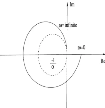
Suppose p(s) has no ju-a,xis roots. Then, the condition (ii) of Theorem 1 has a simple interpretation in terms of the inverse Nyquist plot of p (s )/q {s ) (or the polar plot of q {s)/p {s)). Suppose o: > 0. Then, the condition (ii) of Theorem 1 holds if and only if the inverse Nyquist plot of p {s)/q (s) is contained in the right half plane R e {q(ji^)/p{ji-^)} > —a /2 . Note that if (ii) holds, then the inverse Nyquist plot does not encircle the point { —a ,j0 ) . Applying the inverse Nyquist criterion, in order for condition (i) of Theorem 1 also to hold, it is necessary and sufficient that the polynomial p{s) has no roots in C+, i.e., in the strict right half plane. We thus arrive at the following geometric restatement of Theorem 1. Let p{jco) ^ 0 fo r all a; 6 R . An output feedback
with a > 0 is optim al if and only if p{s) has no roots in the right h alf complex plane and the inverse Nyquist plot o f p {s )/q {s ) is contained in the closed half plane R e ^ —a/2. The inverse Nyquist diagram of a typical system for which a > 0 is optimal is shown in Figure 3.1.
There is yet another equivalent restatement of Theorem 1 in terms of the Nyquist plot of p {s)!q [s). We first note that condition (ii) of Theorem 1 for
a > 0 can be written as
R e { ^ 1 ^ } > - ^ Vo; € R for which q {ju ) ^ 0 (3.4) 2 \q{ju:)y
using the identity
Re { ^ j ^ ] p { j u j ) p { - j u j ) = Re { ^ j ^ ] q { j u ) q { - j u j ) . (3.5) The inequality (3.4) means that, in the ^|^-plane, the Nyquist plot of lies
Figure 3.1: Inverse Nyquist plot for an oiDtimal cv.
outside the open unit disk of radius \ /a and of center ( —l/o;,jO). Using the Nyquist criterion in interpreting the condition (i) of Theorem 1, we arrive at the following geometric criterion for optimality. It is understood that whenever
q{s) has roots on Co, the Nyquist plot is obtained by introducing small semi circles at the Nyquist contour so as to avoid these roots.
C orollary 2 . An output feedback with a > 0 is optimal if and only if
the Nyquist plot o f p {s)/q (s) avoids the open disk o f radius l/cv centered at
{—\ /a ,jO ) and encircles the disk counterclockwise as many times as the number o f -roots o f q{s).
The Nyquist diagram of a typical system for which a > 0 is optimal is shown in Figure 3.2.
E x am p le 1. Consider
P{s) ^ s q{s) «2 _ q. 1 ·
Figure 3.2: Nyquist plot for an optimal a with two C+-roots ol q{s).
We have
f c { ^ ) = B e
p {j^ )
so that all a > 2 are optimal for this system. On the other hand, lor
p{s) _ 5^ + 1 (^,2 + 2)(s + 3)·
MO feedback with a > 0 is optimal since
3(2 -cu^)
r, r'AyyiZi _
{ ^ ■ \ } I
pM 1 - U)^
goes to -o o as a; 1+. Note that condition (i) of Theorem 1 is satisfied tor all cv > 0 since q{s) + ap (s) is Hurwitz stable for all a > 0 by a simple application
of Routh-Hurwitz criterion. *
Figure 3.3: Nyquist plot of ^
Z®
2
Im
Re
Figure 3.4: Inverse Nyquist plot oí ^ — s'^-.v+l '
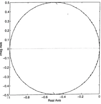
Figure 3.5: Nyquist plot of ^ = (,,2+2)(.U:î) '
Figure 3.6: Inverse Nyquist plot ol — (,2^_2)(s+3)·
3 .2
O ptim ality for second and th ird o rd er
system s
111 this section, we give coefficient conditions on open loop transfer functions of second and third order systems for a given a > 0 to be optimal.
Consider a second order strictly proper transfer function
p{s) _ 6iS + 6o ,2 , , 1,2 _L n
—— — —— ; , «0 ~ bohidi + 7^ 0.
(j{s) S‘‘ + aiS + ao
By Theorem 1, a given a > 0 turns out to be optimal if and only if cii
T
cxbi^ 0
(io + abo > 0
aibi — bo ~l· jb i > 0
do^o + fb^ > 0,
where the first two conditions ensure that q(s) + ap(^>) is Hurwitz stable. Consider a third order strictly proper open loop transfer function
p(s) _ b2s'^ + biS + bp (¡{s) + Cl2S^ + diS + Up
where the resultcint matrix
¿2 bi bp
bi bi bp
62 bi bp
1 CI2 a I dp
1 «2 «1 «0
is assumed nonsingular. Agciin by Theorem 1, a given a > 0 is oiitimal il and only if the following inequalities hold:
dp + abp > 0
«2 + Oib2 > 0 («1 + abx){a2 + 062) — (do + Of&o) > 0
^0^0 + “ ¿0 > 0 a2&2 — + —¿2 > 0
Either , ,2
iiiby + -b\ - «0^2 - boU2 - Cibol)2 > 0 or
1 ^ 1 1
« ■ i b i + — b y - «0^2 - 6o«2 - abob2 < —2^ (ao6o + + ^14)
Following [13], the last “either-or” condition can be replaced by
C-lfh + “ ¿1 — «0^2 ~ bo<^2 ~ O:bob2 — —\j{ilobo + —b>o)iii2b2 — by + — 6.j)
3 .3
P lan ts for which all positive feedbacks are
optim al
We show in this section that the set of open loop systems for whicli all feed backs (3.2) with a > 0 are optimal, are systems having positive real transfer functions. Among the many equivalent characterizations possible for positive realness of (rational) transfer functions, see [7] and Appendi.x C of [18], we use the following as a definition. The definition of strict positive real transfer functions is cittributed to [11].
D efin ition . A transfer function is positive real if it has no poles in C+, the poles with zero real parts (if any) are simple (i.e., have niultipliciti.es
equal to I) with real and positive residues, and
R t { ^ w hich qijw ) ^ 0. (3.6)
/1 transfer function ^ ¿ « strict positive real if q(s) is Hurwitz stable and > 0 Vw e R .
It is well known, [18], [11], that ^ is (strict) positive recil if and only if ^ is. The following lemma simplifies the test lor positive realness.
L em m a 1 . Given a transfer function 4 4 , suppose there exists a > 0 such
that q(s) + ap (s) is Hurwitz stable. Then, ^ is positive real if and only if
(3.6) holds.
P ro o f. Let (3.1) be a reachable and observable realization of the transfer function ^1^. By Proposition 2 of [18], Section L5, if (3.1) is minimally stable, then the second statement of the lemrnci is valid. The system (3.1) is defined to be minimally stable if for every initial state ;f(0), there exists an input u such thcit the solution x{t) of (3.1) satisfies
lirn |);i'(f)|| = 0
6— »-OO (3.7)
and the integral constraint
[ y{t)u{t)dt
Jo
is nonpositive for all > 0. We show that (3.1) is minimally stable under the hypothesis of the lemma. In fact if there exists cv > 0 sucli that q{s) + a p (s) is Hurwitz stcible, consider the input u{t) —a y {t). By Hurwitz stability of
q{s) + «/.»(s) and by the reachability and observability of the plant, the closed loop s}^stem consisting of the plant (3.1) and the feedback —cv is internally
stable. It follows that the solution x{t) of (3.1) is asymptotically stable and hence satisfies (3.7). Moreover, the integral becomes
I
—
a f
y{t)^dt Jo 'which is nonpositive for all ¿1 > 0. Hence (3.1) is minimally stable and the
proof is complete. □
Let us recall a fundamental property of plants with positive real transfer functions. This well-known result follows by Sections 23 and 24 of [18]. VVe give a simple Nyciuist plot argument lor the second statement.
L em m a 2 . A plant with a positive real transfer function is stabilized by
all output feedbacks tc(t) = —a y [t) with a > 0. A plant with a strict positive real transfer function is stabilized by all output feedbacks 'u(t) = —cry(t) with
a > 0.
P ro o f. By Section 24 of [18], it follows that any negative feedback connec tion of two positive real transfer functions gives rise to a “Lyapunov-stable” closed loop system. From the discussion on asymptotic stability in Section 23 of [18] (see condition P of Theorem 1), it follows that if one of the systems is strict positive real, then the closed loop .system is asymptotically stable. This proves both statements. In order to fix ideas, we give the Ibllovving simple Nyquist plot argument for the proof of the second statement.
If the transfer function p {s)/q (s) is sti'ict positive real, then q{s) is Ilurwitz stable so that at cr = 0 the claim is true. Moreover, the Nyipiist plot of
p{s)/q{s) is contained in the open right Imlf p(jijj)/qiju )-p h m c. Hence, tor any cv > 0, the point ( —l/o;,j0) can not be enclosed by the Nyquist plot. By Hunvitz stability of q{s) and by the Nyquist criterion, it follows that q{s) +
crp{s) is Hurwitz stable for all o; > 0. n
The following is the main result of this section.
T h eo rem 2 . All output feedbacks cv > 0 are optim al for the plant (d .l)
and the cost (2.2) if and only if the transfer function ^ is positive real. P ro o f. [If] By Lemma 2, if ^ is positive real, then r/(.s) + ivp(.s) is Hlurwitz stable for all o > 0. Moreover, by the identity (3.5 ), it also follows that > 0 for all u> for which pijuj) 0. Therefore, both conditions of Theorem 1 hold for every o > 0 and all such feedljacks are optimal.
[Only if] By Theorem 1, if all a > 0 cire optimal, then (a) q + a p is Hurwitz stcdale for all cx > 0, and (6) Re {^7^—7} > 0 Vcu G R for which p( ju>) 7^ 0.
By condition (a) and Lemma 1, the transfer function is positive real provided
Re { ^ ^ which q{jeo) 7^ 0. The latter follows by condition (6) cind the identity (3.5). □ R e m a rk s .( 1) We observe from Theorem 1 that a < 0 is optimal for the plant transfer function ^ if and only if —a > 0 is optimal for ~ I f o f this reason, the discussion in the rest of the thesis is restricted to feedl)a.cks (3.2 ) with cx > 0.
( 2 ) It luis been noted in [8] in the multivariable situation that, any output feedback u{t) = —R~^y(t) with R~^ positive definite is optimal with respect to (3.1) and the cost
r [ .T ( 0 '( C 'i ? - ‘ C + Q)x{t) + u{tyRu{t)](lt
Jo
provided the plant is positive real. Although this is a different inverse ])roblem of optimal control as the input penalization matrix ft is assumed unknown, the
result still points out to the optimality property of positive real systems. Our result above applies to scalar systems and to fixed input penalization R = 1. It also provides a converse to the result of [8], namel}^, if all positive cv > 0 are optimal for a plant, then the plant must be positive real.
C o ro llary 3. Let p{juj) ^ 0 /or all co G R . Then, all output feedbacks
nd (2.2) if o f (S. 1) is strict positive real.
a > 0 are optim al fo r (3.1) and (2.2) if and only if the transfer function ^
P ro o f. If the transfer function p {s)fq (s) is strict positive real, then, by Lemma 2, q(s) + ap (s) is Hurwitz stable and, by (3.5), Re > 0 > —a /2 for any Q; > 0. By Theorem 1, we have that any cv > 0 is optimal for the plant (3.1) and the cost (2.2). Conversely, if all a > 0 are optimal, then, by Theorem 2 considering a > 0, the transfer function is positive real and, by the hypothesis, p{s) is Hurwitz stable. By Theorem 1 considering « = 0, the polynomial </(s) is also Hurwitz stable. By continuity of 44^ with respect to CO, it follows that Re > 0 for all a; G R and p{s)l(i[s)
is strict positi
real.
ive
□
3 .4
M inim um phase system s
In this section, a class of feedbacks optimal for a class of minimum sj^stems are determined as an application of Corollary 3. We first show that under a preliminary (usually high gain) feedback, a minimum phase system of the type defined below can be made strict positive real. Any feedback
u[t) = —a y (t) with cv larger than two times the value of this preliminary feedback is then shown to be optimal for the original minimum phase [)Iant.
We first adopt a “non-standard” definition.
D efin itio n . A strictly proper plant o f transfer function 4 4 will be called s tr ic t m inim um phase if p{s) is Hurwitz stable, deg p(s) = deg q{s) — 1, and
the highest coefficients o f p{s) and q{s) are o f the sam e sign.
L em m a 3. Given a strict minimum phase there exists k > 0 such that P(^)
q(s) -i- Sp{s)
is strict positive real fo r all S > k.
P ro o f. Let us assume without loss of generality that the highest coefficients of p(s) and q(s) are both positive. Since p{s) is Hurwitz stable and d eg p =
deg q — 1, by root-locus considerations it is easy to see that there exists / > 0 such that r(s) := q{s) -b ^p{s) is Hurwitz stable for all ¡3 > 1. In what follows, we show that there exists ^ > 0 such that p(s)/[r(s) -f 7^(5)] is strict positive real for all j > k. From this it easily follows that p(s)/[q'(s) -|- 0 ^(3)] is strict positive real for all a > A; -f /. The transfer function p(s)/[r(s) -f 7p(a·)] is strict positive real if and only if
R e {r {ju ;)p (-ju j)} -|- 7P (i‘^)p(“ i^ ) > 0 V w G R . (3.8) Since both r{s) and p{s) are Hurwitz stable, all coefficients are nonzero and of the same sign (see e.g., [7]). By our assumption that the highest coefficients of
q{s) and p{s) are positive and by d eg p {s) = deg q{s) — 1, d eg q(s) = d e g r {s ), it follows that all coefficients of r(s) and p{s) are positive. Hence the following equality holds for the degrees in or.
deg^Re { r { jo j) p { - ju ) } = d eg ^ p{joj)p{-joj).
Since
> 0 Va> e R ,
= +
00,
there exists a suitable A; > 0 such that for ¿ill 7 > k the inequality (-1.8 ) is satisfied. Therefore, the transfer function
p(^)
r{s) + 7p(s‘)
is sti’ict positive real for all 7 > ^ since it has a strict positive real part at •s· = juj and p{s) (and ?’(s) + ‘jp is )) is Hurwitz stable. □
T h eo re m 3. Given a strict minimum phase plant (S .l), let k > 0 he such
that the closed loop system o f Figure S .l is strict positive real fo r all 8 > k.
Then, every a > 2k is optimal fo r (3.1) and (2.2). P ro o f. A preliminary feedback k > Q such that
p(·^) (/(.s) + 8p{s)
is strictly positive real for all 8 > k exists by Lemma '■]. By definition of strict positive realness, the denominator polynomial f/(.s) + 8p(.s) is Ilurvvitz stable for all 8 > k, and also using (3.5), we have
Re { --- —---} > 0
p{j^ )
for cill 8 > k. This yields
and </(s) + ap(s) is Hurwitz stable. Therefore, by Theorem 1, a is o|)timal for
□
P( s )7
(s) ■
R e m a rk . Although the discussion above has been restricted to strictly proper plants, all the results above have appropriate extensions to the more general case of a single-input, single-outi^ut phmt
(3.9)
x{t) = Ax{t) + B u (t), ;c(0) = .To,
y{t) = C x(t) + Du(t) with an output feedback
u{t) = - a y { t ) , (;}.10)
where a G R . We call a feedback (3.10) optimal for the plant (3.9), and the cost (2.2) if (i) 1 + a D Ф 0 and (ii) the corresponding state feedback н(/) = — A'.r(/) with
К a -C
1 + aD
is optimal for (3.9) and the cost (2.2). The condition (i) is includoxl for the closed loop system to be well-defined. Since the statement of the results for this more general case are slightly more involved (mainly due to the nonlinear dependence of K on a), we have restricted our discussion to strictly propi'r plcuits (D =0).
C hapter 4
A PPLIC A T IO N S
Here, we examine one mechanical and one electro-mechanical .system with the application of the results of Chapter 3 in mind. The second example, stepping motor, is a particularly difficult case since its transfer function is far from being positive real. We examine the possibility of ciltering the translhr function by a feedforward compensation so that it becomes positive real for some values of the motor constants.
4 .1
A utom obile suspension system
Figure (4.1) shows a schematic diagrcun of an automobile suspension system. The linearized equation of motion for this standard textbook example, [15], is obtained as follows.
.A.S the car moves along the road, the vertical displacement of the tiix's act as the motion excitation to the automobile suspension system. The motion of this system consists of a translational motion of the center of mass, indicated
mxo + h{xo - Xi) + k{xo - a;,·) = 0 or
in the figure as m. The equation of motion for the system is;
mxo + bxo + kxo = hxi + kxi
(4.1) (4.2) Assuming that the motion Xi at point P , which is the center of mass of the tires, is the input to the system and the vertical motion Xo of the body is tlie output, considering the motion of the body m only in the verticcil direction, we obtain the transfer function as:
X ois) hs -f- k
(4..4)
X i{s) ms'^ + bs + k
For this second order transfer function, the coefficient condition in Section 3.2 can be applied verbatim on setting
bi = ai = — , 6o = «0 = — .
m rn
Furthermore, all feedbacks with a > 0 are optimal for this transfer function, i.e., the transfer function is positive real (Section 3.2.1) if and only if
b^ > m k. (4.4)
4 .2
Stepping m otors
'Fhe following description and the linear model of a stepping motor is adapted from [14]. DC motors are devices which converts an electrical input into a mechaniccil motion. Stepping motors can perform the same or similai· functions with the following significant advantages;
• No feedback is usually required for either position or speed control.
• positional error is noncumulative, and
• stepping motors are compatible with modern digital equipment.
(
Here we examine the Two Phase Variable Reluctance (VR) voltage driven step ping motor. The transfer functions of other types of stepping motors have the same structure. Consider the model of a VR motor shown in Figure 4.2, where A is the pitch angle and Oi is an equilibrium position. An equilibrium position is a rncignetic null obtained by circulating nominal steady state currents through the windings of the stator. It was found that a very small displacement of this magnetic null around the stepping position can be obtciined by applying differential currents to the same windings of the stator. Let us now define the desired position as the magnetic null where the load is to be fine positioned by the motor. Magnetic null is obtained b}^ interaction of the rotor motion in order to reduce the reluctance and the magnetic fields of the excited windings. The equation of motion of the rotor is
, (PO ^ dO ^ ^
+ Dair~^ + Ti -|- T); — 0, (4.5) where ,1^ is the inertia of the rotor, 0 is the actual position of tlu' rotor, Dai,· is the viscous damping coefficients of the air and friction, T,, is the tor((ue due to current in phase A and 7), is the torque due to current in phase B. Tlie expressions for Ta and Ti, are:
Ta = p^,nibSin{pO) (4.6)
Tb = p<if,niaSin{p{0 - A)), (4.7) where p is the number of pairs of magnetic poles, is the flux, A is the pitch angle, is the current in phase A and ib is the current in phase B. The
electrical equations neglecting the mutual inductance are: = ria + + '^^h'>'^m('Os{Nr0)) r dll d , ^ Vb = rib + L — + — (n$,„A·г7г(A^,.d)), (4.8) ( 1 . 9 )
where r is the winding resistance and Nr is equal to p. For proper positioning of the rotor, magnetic damping and mechanical damping are used. If we comiect a mechanical damper to the rotor, the equation of motion is changed as;
r.d0 rr. rr.
(1.10)
where Td is the viscous torque exerted on the damper housing, J is the ec(ui vio lent inertia of the rotor and the damper housing and D is the viscous diirnping coefficients of the air, friction and damper. The expression for Td is obtained from
rlf) rp f) I
(4.11)
dO dOdo^ j (POdo
where Dd is the viscous damping coefficient of the damper, Odo is the position of the inertial flywheel, and Jdo is the inertia of the damper housing. Using the last four equations, after linearizing, we obtain the following transfer function
0 ( . s ) b\S + 6()
H {s) = ( 4 . 1 2 )
K (s) - K(-5) + a2S^ + (iiS + «o’
where K,(.s) and H(-s) are the Laplace transforms of the applied voltages at phases /1 and 5 , respectively, and where
(ii\ — JinddoP JdiddoP
ri;3 —
djnddo'^'4”
Jindd^dd/T
Jdodd^djT
ddiddo^T
ddidddd-^“b 'L/o44f/Z/
« 2 = J m d )d > ' Jd o d d d i' -l· D D d L + J d i D d V + C iJ d o d j + Jd o d )d > ' +
s m ( — ) { s t n { - ^ ) - cos{— ))NrJdo
Ol = D D d T c ı J d o T + cıDdLp<^l^ri^sin{^^^){sin{^^) - cos{^^^))NrDd2i 2i 2 00 = CxDdV h = P ^ m n sİn {^ ^ )Jd o 1 X . ' / ^ \ 1-» Oo = p9ynnstn{—^ ) D d Cı = 2p^^rnnIoCOs{^^).
A positive a is optimal for H {s) provided the following conditions are satisfied by the coefficients:
0 < 04 0 < 03
0 < 0302 — 04(01 + a b i)
0 < [03O2 — 04(01 + o;öı)](oı + Cibi) — 03(00 + cxbo)
0 <C oqa ocbo
0 < (0460- 0361)
0 ^ 2o i6i "b 0:61 — 20260 0 ^ 2oo6o + oii>Q
The last three conditions are sufficient to satisfy the condition (ii) of Theorem 1. The first two conditions automatically hold.
Since H {s) has relative degree 3, it is not positive real irrespective of the values of its coefficients. Let us now suppose that a precompensator is added in the feedforward path as shown in the block diagram at Figure 4.3. We assume that a precompensator of derivative type is used. More specifically, linearized precompensator is assumed to have a transfer function of the form
H i{s) = as^ + b. (4.13)
( 4 . 1 4 )
So the overall transfer function of the precompensator and the motor becomes , , 0 ( s ) ct,b\s^ 4“ cib(jS^ -h bb\s -|- bb{)
E{s) a.iS'^
+
a:is'·^+
ii2s'^+ «i -s +
Uo’
A positive a is optimal for H is) provided the following conditions hold.
0 < —‘¿aa^bo + 2 0 0 3 6 1 + aa^b\
0 < 204660 + 200260 — 203661 — 2ooi6i +
acEbg — 2(xabb\0
^ —
o o q6
o— O2660 4“
ci\ bbi4“ oi6^6| —
2 омЬЬ^0
<
2oo
66o
4-
(xb^b^ 0< 03
4-
(xcibi0 < oo 4- abbo
0
< (03
4-
a a 6i)(o2 4-
ao6o)- 04(01
4-
« 661)0
< [(03 4-
«o 6i)(o2 4-
«або)- 04(01
4-
rv66i)](oi 4-
rv66i)— (03
4-
O!o6i)(oo 4-
(xbbo)furthermore, the transfer function Н {з) is positive real and theretore any cv > 0 is optimal provided о and 6 are so chosen that:
0 < 0302 — 04O1 0 < 01(0302 — «4« i) — ao«3 0
< 00361 — 00,460
0< 00260
4- 04660 — 00161 — 03661
0 < о 1661 — ООобо — O2660 О < ооббоThe hict that stepping motors hardly need feedback compensation lor position control indicates that the denominator polynomial of //(.s) has stalrle [)oles for realistic values of the parameters o*. Hence, it may be possible to satisfy
the above set of inequalities for a wide range of stepping motors by a suitable choice of a and b.
Figure 4.1: Automobile suspension system.
Figure 4.3: Feedback configuration for the precornpensated motor.
C hapter 5
CON CLUSION S
From our investigation of systems for which some or all positive constant output feedbacks are optimal emanates the positive realness conditions in Theorems 1 and 2. As expected, generally high gain feedbacks turn out to be optimal for minimum phase systems and small gain feedbacks may not be optimal or even stabilizing. This follows from Theorem 3 and Theorem 1.
The fields of optimal control and positive real systems both being very old and well investigated, all these results are probably known in some form or other. What may be new is the focus of attention at the optimality of an output feedback. The connection between optimal constant output feedbacks and the property of positive realness seems to be either newly being noticed or being rediscovered, [8].
We have only considered scalar, continuous-time, strictly proper systems leaving the pursuit of the extensions to more general situations for future work.
R E F E R E N C E S
[1] B. D. 0 . Anderson, “The inverse problem of optimal control”, Rep. SEL-
66-039, Stanford University, Stanford, CA, 1966.
[2] B. D. 0 . Anderson and J. B. Moore, Linear Optimal Control, Prentice Hall, Englewood Cliffs, New .Jersey, 1971.
[.3] B. D. 0 . Anderson, S. Dasgupta, P. Khargonekar, F. J. Kraus, and M. Mansour, “Robust strict positive realness: Characterization cind construc tion”, IE E E Transactions on Circuits and Systems, vol. 37, no. 7, pp. 869-875, July 1990.
[4] H. Chapellat, M. Dahleh, and S. P. Bhattachciryya, “On robust nonlinear stability of interval control systems”, IE E E Transactions on Automatic
Control, vol. AC-36, pp. 59-67, Jan. 1991.
[5] T. Fuji! and M. Narazaki, “A Complete Optimality Condition in the In verse Problem of Optimal Control”, SIAM J. o f Control and Optimization, vol. 22, No. 2, pp. 327-341, March 1984.
[6] T. Fuji! and M. Narazaki, “A Complete Optimcdity Condition in the In verse Problem of Optimal Control”, Proc. o f 1982 IE E E Conference on
Decision and Control, pp. 289-294,
[7] F. R. Gantmacher, The Theorxj o f M atrices, Vol. I f New York: Chelsea Publishing Company, 1959.
/
[8] .J. D. Gardiner, “Stabilizing Control for Second Order Models and Positive Real Systems”, Journal o f Guidance, Control, and Dynamics, vol. 15, No. 1, pp. 280-282, Jan.-Feb. 1992.
[9] E. A. Guillemin, Synthesis o f Passive Networks, .John Wiley and Sons, New York, 1957.
[10] D. C. Plyland, W. M. Haddad, and V-S. Chellaboina, “Frequency domain performance bounds for uncertain positive real systems”. Journal o f Guid
ance, Control, and Dynamics, vol. 19, No. 2, pp. 398-406, March-April 1996.
[11] E. I. .Jury, Inners and Stability o f Dynamic Systems, New York: Wiley, 1974
[12] R. E. Kalman, “Contributions to the theory of optimal control”, Bol. Soc.
Mat. Mexicana, pp. 102-119, 1960.
[13] R. E. Kalman, “When Is a Linear Control System Optimal?”, Jou rn al o f
Basic Eng. Trans, o f the ASME, pp. 51-60, 1964.
[14] T. Kenjo, Stepping Motors and their M icroprocessor Control, Clarendon Press, Oxford, 1984.
[15] B. C. Kuo Automatic Control Systems, Prentice Hall International, 1991 [16] W. S. Levine and M. Athans “On the determination of the optimal con
stant output feedback gains for linear multivariable systems”, IE E E Trans.
Automatic Control, vol. AC-15, No. 1, Feb. 1970.
[17] A. B. Özgüler “Phase growth conditions and their applications in strict positive real design problem”, working paper, Bilkent University, Electrical
and Electronics Engineering, Bilkent, Ankara, 06533, Turkey, 1996. [18] V. M. Popov, Hyperstability o f Control Systems, Springer-Verlag, 1973. [19] A. Rcintzer, “Stability conditions for polytopes of polynornicils”, IE E E
Trans. Automat. Contr., Vol. 37, pp. 79-89, 1992
[20] .1. L. Willems, Stability Theory o f Dynamical Systems, Nelson, London, 1970.