Phase retrieval of sparse signals from Fourier Transform magnitude using non-negative matrix factorization

Phase Retrieval of Sparse Signals from Fourier

Transform Magnitude using Non-Negative Matrix

Factorization

Mohammad Shukri Salman, Alaa Eleyan

Electrical and Electronic Engineering Department Mevlana University

Konya, Turkey

{mssalman, aeleyan}@mevlana.edu.tr

Zeynel Deprem , A. Enis Cetin

Bilkent University Ankara, Turkey

cetin@bilkent.edu.tr, zdeprem@ee.bilkent.edu.tr Abstract—Signal and image reconstruction from Fourier

Transform magnitude is a difficult inverse problem. Fourier transform magnitude can be measured in many practical applications, but the phase may not be measured. Since the autocorrelation of an image or a signal can be expressed as convolution of with , it is possible to formulate the inverse problem as a non-negative matrix factorization problem. In this paper, we propose a new algorithm based on the sparse non-negative matrix factorization (NNMF) to estimate the phase of a signal or an image in an iterative manner. Experimental reconstruction results are presented.

I. INTRODUCTION

Magnitude of the Fourier transform of a desired signal or an image can be measured or calculated in many practical problems ranging from astronomical imaging to crystallography. However, it may not be possible to measure the phase information. This inverse signal reconstruction problem is a difficult one and a wide range of algorithms have been proposed in the literature [1]-[12]. The inverse problem is especially difficult when the magnitude values are corrupted by noise.

It is well known that when the desired signal is one dimensional and it consists of samples the phase retrieval problem has 2 to the solutions. When the signal has two or more dimensions the solution is unique in almost all cases [12]. The main reason for this difference between the 1-D and higher dimensional problems are that the fundamental theorem of algebra cannot be extended to higher dimensions.

In this article we assume that the desired signal is a discrete signal and its Fourier Transform is available for all frequency values. We also assume that: (i) the signal is non-negative, (ii) sparse in time or spatial domain, and (iii) finite-extent, i.e., it consists of N samples in 1-D, and it consists of N×N samples. Sparsity is also assumed by Eldar et al. [15] Non-negativity of the signal samples were used by Fienup and his co-workers. In almost all image processing problems pixel values are positive therefore the non-negativity assumption is not a restrictive assumption.

In this article, the nonnegative matrix factorization (NNMF) algorithm and its sparsified version [13], [14] are used to solve the phase retrieval problem. Since the inverse Fourier Transform of the squared magnitude is the autocorrelation sequence of the desired signal it is possible to formulate the phase retrieval problem as a non-negative matrix factorization problem. In Section 2, the NNMF based algorithm is described. In Section 3, simulation examples are presented.

II. PHASE RETRIEVAL PROBLEM

Let , 0, 1, 2, . . . , 1be the signal to estimated. The Discrete Fourier Transform (DFT) of the signal is given by

∑

.

The Fourier Transform magnitude | | information is equivalent to the autocorrelation sequence of the signal. This is because

| | , (2) where * is the convolution operator and . denotes the inverse Fourier Transform. This also can be represented using matrix multiplication as 0 1 1 0 1 2 1 0 0 3 2 0 0 0 0 0 1 1 , (3)

where 0 1 1 is the autocorrelation

sequence and 0 1 1 is the input

signal. As a result the autocorrelation sequence can be represented as:

, (4)

where and are defined in Eq. (3), respectively. In phase retrieval problems, it is assumed that the autocorrelation vector r is known but and are unknowns.

Therefore it is possible to apply the NNMF algorithms to estimate and .

1113

III. NON-NEGATIVE MATRIX FACTORIZATION ALGORITHM

Non-negative matrix factorization (NNMF) algorithms [13], [14] estimate the non-negative matrices and from the matrix by minimizing the norm

of .

The error function has a convex behavior once W or H is known. However, there may be many local minima in the general matrix factorization problem.

The NNMF algorithm proposed by Lee and Seung [13] starts with an initial solution. First one of the matrices is estimated. Once this matrix is fixed this matrix is used to update the second matrix. The iterative algorithm is described below: rand M, rand , N iteration { }, (5)

This algorithm by its nature continuously generates negative matrices when it is started with matrices with non-negative entries. But if one of the entries of one of the matrices happens to be zero iterations stop. Another update method is the “Alternative Least Squares (ALS)” method. The ALS algorithm is summarized as follows:

rand M, iteration { 0 0 0 0}, (6) Here, there could be a problem due to the matrix inversions in the first and third lines of the algorithm if some elements of the matrices are below zero. Those negative entries are thresholded to zero. Also, sparsity assumption can be imposed into this method by simply making small valued entries to zero. This is done at the second and fourth lines of the ALS algorithm (6). Furthermore, ALS method assumes that the matrices to be inverted are non-singular at each iteration. There are other sparsified nonnegative matrix factorization algorithms exist in the literature [14].

IV. APPLYING NNMFALGORITHM TO AUTOCORRELATION

FUNCTION

One of the key points to keep in mind while estimating the desired signal is that both matrices and are dependent to

each other in autocorrelation factorization problem. This dependency should be maintained during the update steps of the iterative NNMF algorithms. Another important issue is that the ALS method given in (6) cannot be applied directly to our problem because has a rank of 1 and its inverse does not exist.

However, due to the dependency between the variables and the sparse nature of the signal, a new update method can be developed as follows: 1 1 1 iteration { 0 0 0 / } (7)

As pointed above our algorithm described in (7) is different from the ALS algorithm (6). One can start with different initial condition vectors. Iterates may converge to different solutions depending on the initial estimate.

Extension of this algorithm to two- or higher dimensions is straightforward.

V. SIMULATIONS AND RESULTS

In order to test the performance of the algorithm, a 1-dimensional example is provided in Table I. The signal to be reconstructed from its spectrum is assumed to be of length 16. TABLE I.EXAMPLE 1 12.00 12.00 189.00 189.00 0.00 0.00 0.00 0.00 0.00 0.00 8.00 8.00 0.00 0.00 0.00 0.00 0.00 0.00 0.00 0.00 0.00 0.00 20.00 20.00 0.00 0.00 0.00 0.00 0.00 0.00 10.00 10.00 5.00 5.00 60.00 60.00 0.00 0.00 0.00 0.00 0.00 0.00 0.00 0.00 0.00 0.00 0.00 0.00 0.00 0.00 0.00 0.00 4.00 4.00 48.00 48.00 0.00 0.00 0.00 0.00 2.00 2.00 24.00 24.00 1114

In example 1, it is clear that the original signal and its autocorrelation sequence are successfully reconstructed. In general, there are 2 solutions for a given autocorrelation sequence in 1-D case but it is possible to recover the original signal in a perfect manner by imposing sparsity in this toy example.

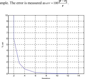
Fig. 1 shows the convergence curve of the aforementioned example. The error is measured aserr=100 r r−ˆ

r .

Figure 1. Convergence behavior of the proposed algorithm for example 1.

(a) (b)

(c)

Figure 2. (a) Original image, (b) autocorrelation image, (c) Reconstructed image.

In order to test the performance of the proposed algorithm in two-dimensional case, 1 experiment without noise and 2 experiments with different noise variances were conducted using the sparse images given in Fig. 2(a), Fig. 3(a) and Fig.

4(a). All the images used in the experiments are of size (136 136).

Fig. 2(a) shows the original sparse image, Fig. 2(b) shows the autocorrelation function of the noisy image and Fig. 2(c) shows the reconstructed image from the spectrum of the original image. It is clear that the main details of the original image can be reconstructed from its spectrum using the proposed algorithm.

(a) (b)

(c) (d) Figure 3. (a) Original image, (b) Image with AWGN noise

0.001 , (c) Image autocorrelation, (d) Estimated image.

(a) (b)

(c) (d) Figure 4. (a) Original image, (b) Image with AWGN noise

0.005 , (c) Image autocorrelation, (d) Estimated image.

2 4 6 8 10 12 14 0 1 2 3 4 5 6 7 8 9 10 Iteration % e rr 1115

In Fig. 4, the AWGN is assumed to be with zero mean and normalized variance 0.005 . Even though the noise variance is high compared to the first experiment, but the algorithm is still capable of reconstructing the main details of the original image.

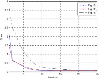
Figure 5. Convergence behavior of the proposed algorithm for images in Figs. 2, 3 and 4.

Fig. 5 shows the convergence curves for the experiments in Figs. 2, 3 and 4. It shows that the performance of the experiments for Figs. 2 and 3 have fast convergence and lower error than that of the one in Fig. 4. This is due to the nature of the image and its sparsity. On the other hand, the convergence of Fig. 2 to steady state is faster than that of Fig. 3. This shows the effect of the noise on the performance.

As it can be seen from the above examples, a sparse signal can be estimated to some extent from its Fourier Transform magnitude or from its autocorrelation using the NNMF methods. It is well-known that the phase retrieval problem is an ill-posed inverse problem in nature therefore the reconstruction results are not perfect even in noise-free cases. The proposed phase retrieval algorithm is a convergent algorithm because the NNMF algorithm is also a convergent algorithm but it may converge to a local minimum.

VI. CONCLUSIONS

In this paper, a new class of phase retrieval algorithms using iterative NNMF algorithms is introduced. The phase retrieval problem can be formulated using a matrix factorization problem with the help of the autocorrelation function of the desired signal. Any NNMF algorithm can be used to solve the phase retrieval problem. However the

problem is an ill-posed problem therefore noise or numerical inaccuracies may lead the iterations to a local minimum.

ACKNOWLEDGEMENT

A. Enis Cetin was supported by Turkish Scientific Research and Technical Research Council (TÜBİTAK) project No. 111E057

REFERENCES

[1] J. R. Fienup, “Phase retrieval algorithms: a comparison,” Applied Optics, vol. 21, no. 15, pp. 2758-2769, 1982.

[2] R. W. Gerchberg and W. O. Saxton, “A practical algorithm for the determination of the phase from image and diffraction plane pictures,”

Optik, no. 35, no. 2, pp. 237-246, 1972.

[3] W. O. Saxton, Computer Techniques for Image Processing in Electron Microscopy, Academic Press, New York, 1978.

[4] M. H. Hayes, J. Lim, A. V. Oppenheim, “Signal reconstruction from phase or magnitude,” IEEE Transaction on Acoustics, Speech and Signal

Processing, vol. 28, no. 6, pp. 672-680,1980.

[5] A. Enis Cetin, R. Ansari, “Convolution-based framework for signal recovery and applications,” Journal of Optical Society of America- A, vol. 5, no. 8, pp. 1193-1200, 1988.

[6] D.C. Youla, H. Webb, “Image Restoration by the Method of Convex Projections: Part-1 Theory,” IEEE Transactions on Medical Imaging, vol. 1, no. 2, pp. 81-94, 1982.

[7] M. I. Sezan, H. Stark, “Tomographic image reconstruction from incomplete view data by convex projections and direct Fourier inversion,” IEEE Transactions on Medical Imaging, vol. 3, no. 2, pp. 91-98, 1984.

[8] M. I. Sezan, H Stark, “Image restoration by the method of convex projections: Part 2-Applications and numerical results,” IEEE

Transactions on Medical Imaging, vol. 1, no. 2, pp. 95-101, 1982.

[9] S. Alshebeili, A. E. Cetin, “A phase reconstruction algorithm from bispectrum,” IEEE Transactions on Geoscience and Remote Sensing, vol. 28, no. 2, pp. 166-170,1990.

[10] N. C. Gallagher and B. Liu, “Method for Computing Kinoforms that Reduces Image Reconstruction Error,” Applied Optics, vol. 12, pp. 2328-2335, 1973.

[11] E.J. Candes, Y. C. Eldar, T. Strohmer and V. Voroninski, “Phase retrieval via matrix completion,” Arxiv preprint arXiv: 1109.0573, pp. 1-24, 2011.

[12] M. H. Hayes, J. H. McClellan, “Reducible polynomials in more than one variable,” Proceedings of the IEEE, vol. 70, no. 2, pp. 197-198, 1982. [13] D. D. Lee, H. S. Seung, “Algorithms for non-negative matrix

factorization,” In T. K. Leen, T. G. Dietterich, and V. Tresp, editors, Advances in Neural Information Processing Systems 13, pp. 556–562. MIT Press, 2001.

[14] P. O. Hoyer, “Non-negative Matrix Factorization with Sparseness Constraints,” Journal of Machine Learning Research, vol. 5, pp. 1457-1469, 2004.

[15] Y. Shechtman, A. Beck and Y. C. Eldar, “Efficient Phase Retrieval of Sparse Signals,” IEEE 27th Convention of Electrical & Electronics

Engineers in Israel (IEEEI), pp. 1-5, November 2012.

5 10 15 20 25 0 0.5 1 1.5 2 2.5 3 3.5 4 Iteration % e rr Fig. 2 Fig. 3 Fig. 4 1116