Multiscanning mode laser scanning confocal microscopy system

© TÜBİTAK

doi:10.3906/elk-1807-268 h t t p : / / j o u r n a l s . t u b i t a k . g o v . t r / e l e k t r i k /

Research Article

Multiscanning mode laser scanning confocal microscopy system

Department of Electrical and Electronics Engineering, Faculty of Engineering, İstanbul Bilgi University, İstanbul, Turkey

Received: 25.07.2018 • Accepted/Published Online: 10.12.2018 • Final Version: 22.03.2019

Abstract: In this paper, a table-top, reflective mode, laser scanning confocal microscopy system that is capable of scanning the target specimen alternately through various scanning devices and methods is proposed. We have developed a laser scanning confocal microscopy system to utilize combinations of various scanning devices and methods and to be able to characterize the optical performance of different scanners and micromirrors that are frequently used in scanning microscopy systems such as multiphoton microscopy, optical coherence tomography, or confocal microscopy. By integrating the scanner to be characterized on the same optical path with a galvanometric scan mirror, which is the conventional benchmarking scanning unit in a typical scanning microscope, we obtain two major advantages: (1) microscopy images are automatically acquired from the same location on the target specimen without having any time-consuming alignment problem and accordingly provide a high-quality optical comparison opportunity, and (2) it totally eliminates the utilization of a second scanning microscopy to benchmark the performance of the scanner-based system and considerably reduces the time spent for imaging, which is a crucial factor for a freshly excised tissue, especially under a fluorescence microscope. The system is composed of a 658 nm laser source, collimation optics, a 2D galvanometer, a 2D polymer micro-scanner, an objective lens with a numerical aperture of 0.40, a 100 µm pinhole, a PMT, a DAQ card and peripheral electronics as well as a Matlab software that simultaneously controls the system through a personal computer. Prototype of the proposed flexible LSCM system is first optically characterized using a USAF resolution target. Subsequently, we provided images of red blood and bacteria cells to demonstrate the systems’ capability for clinical diagnostics. It is reported that maximum FOV and lateral resolution of the proposed LSCM are measured to be 420 µ m x 360 µ m and 1 µ m with galvanometer and, and 117 µ m x 117 µ m and 3.2 µ m with the polymer scanner unit, respectively.

Key words: Laser scanning confocal microscopy, skin cancer, polymer scanner, galvanometric scan mirrors, raster scanning, Lissajous scanning, benchmarking

1. Introduction

Laser-scanning confocal microscopy (LSCM) is an optical imaging technique that enables three-dimensional (3D) imaging of biological cells and tissues thanks to its optical sectioning capability, which is a noninvasive technique that grants the collection of the tissue images, layer by layer, without resorting to any kind of physical slicing [1–11]. Reflective-mode LSCM scans a target sample point-by-point with a laser beam in a sequential way [12]. It epi-collects the reflective incident light coming from the focused specimen, passes it through a spatial filter that is located at the other focusing point of the microscopy system, and feeds it to a transducer to convert the light intensity data to corresponding voltage values. It later employs these acquired pixel information and

digitally assembles them into a meaningful image [13]. By repeating this procedure and automatically collecting light intensity information from different z-slices of the tissue, LSCM eases the noninvasive imaging of living specimens [14].

LSCM technique has some major advantages over conventional optical wide-field microscopes. It allows imaging of living tissue in depth, up to 1 mm, by scanning the target sample in narrow slices, resulting an image with a narrow depth of field, as low as 0.1 mm. This feature of LSCM allows taking images from various depths of the sample to build a 3D image set. The operator can manipulate and measure certain structures in the sample 3D image. The other advantage of the LSCM is that it can have a very high resolution and enables real time in vivo imaging of the targeted specimen. It has been reported that the LSCM can measure details down to 100 nm [14]. Moreover, LSCM can also be implemented in a very simple and compact manner [15,16] and can function as a portable hand-held device [17,18].

There are well-established scanning methodologies used in scanning microscopy such as raster scanning [19], Lissajous scanning [21,30], free-line scanning [22], rotational scanning [23], and spiral scanning [24]. In the raster scanning scheme, resolution of the acquired images is directly related to the ratio of orthogonal scanning frequencies [25,26]. Though the raster scanning pattern is comfortably preferred for Si microscanner-based imaging systems [27] as in the case of standard galvanometric scan mirrors, a Lissajous scanning pattern is adopted in laser scanning systems where attaining high-resolution values is impractical due to low fast-to-slow scan frequency ratio of the utilized scanning device [21, 28, 29]. In this work, we have developed a laser scanning confocal microscopy system to utilize combinations of various scanning devices and methods. Using the proposed setup, we will be able to characterize the optical performance of different scanners and micromirrors that are frequently used in scanning microscopy systems such as multiphoton microscopy, optical coherence tomography, or confocal microscopy. The proposed system contains two different scanning units: (1) a conventional two-dimensional (2D) galvanometric scan mirror and (2) a 3D printed polymer scanner. By integrating the scanner to be characterized on the same optical path with a galvanometric scan mirror, which is the conventional benchmarking scanning unit in a typical scanning microscope, we obtain two major advantages: (1) microscopy images are automatically acquired from the same location on the target specimen without having any time-consuming alignment problem and accordingly provide a high-quality optical comparison opportunity, and (2) it totally eliminates the utilization of a second scanning microscopy to benchmark the performance of the scanner-based system and considerably reduces the time spent for imaging, which is a crucial factor for freshly excised tissue, especially under a fluorescence microscope.

The implemented system is composed of a laser source with a wavelength of 658 nm, various collimation optics, a 2D galvanometric scan mirror, a magnetically actuated 2D polymer scanner, an objective lens with a numerical aperture (NA) of 0.40, a 100 µ m pinhole, a photomultiplier tube (PMT), a data acquisition card (DAQ card), and peripheral electronics, as well as MATLAB software that simultaneously controls the system through a personal computer. The prototype of the proposed flexible LSCM system is first characterized using a US Air Force (USAF) resolution target and then fully tested by imaging numerous tissue and cell samples.

This paper is organized as follows: in Section 2, the proposed LSCM system is elaborated. Subsequently, in Section 3, details on system implementation and image construction methodology are shared. Experimental results and images acquired with the proposed LSCM system are given in Section 4. Finally, the report is finished with a summary and discussion in the concluding section.

2. System description

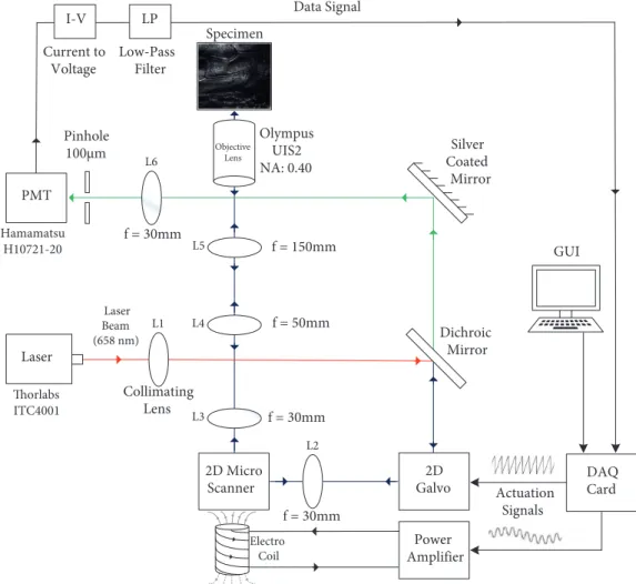
The block diagram of the proposed multiscanning-mode laser-scanning confocal microscopy system is shown in Figure1. We implemented a system composed of a Thorlabs-LP660-SF60 60 mW laser source with a wavelength of 658 nm, an optical lens setup, a Hamamatsu-H10721-20 photo-multiplier tube (PMT), an NI-USB 6356 data acquisition card (DAQ), a two-dimensional (2D) polymer-based laser scanner, and a Thorlabs-GVS002 2D galvanometric (galvo) scan mirror.

Laser Beam (658 nm) Actuation Signals GUI Data Signal 2D Micro Scanner f = 30mm f = 30mm f = 50mm f = 150mm f = 30mm Dichroic Mirror Silver Coated Mirror Olympus UIS2 NA: 0.40 Pinhole 100µm Collimating Lens Thorlabs ITC4001 Hamamatsu H10721-20 Specimen Laser DAQ Card Power Amplifier Objective Lens 2D Galvo Electro Coil PMT L2 L3 L1 L4 L5 L6 I-V LP Low-Pass Filter Current to Voltage

Figure 1. System diagram of the implemented laser-scanning confocal microscopy system. Distances between compo-nents: laser-to-L1 is 30 mm, 2D microscanner-to-L2 is 25 mm, L2-to-2D galvo is 35 mm, 2D galvo-to-dichroic mirror is 100 mm, dichroic mirror-to-silver coated mirror is 125 mm, 2D microscanner-to-L3 is 35 mm, L3-to-L4 is 50 mm, L4-to-L5 is 200 mm, L5-to-objective lens is 350 mm, and L6-to-PMT is 30 mm.

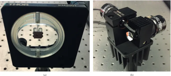
The system incorporates two different laser-scanning devices: one conventional off-the-shelf 2D galvano-metric scan mirror to be used for benchmarking and a 2D polymer scanner to be compared with the galvanometer with respect to its optical performance. These devices, which are shown in Figures 2a and 2b, can be inter-changeably used as the laser steering device in the system together with the preferred scanning method being raster or Lissajous scanning patterns.

The scanning device and the method can be adjusted on the microscope using the graphical user interface depending on the specimen under observation, target FOV, and FPS. The proposed system can either scan the targeted specimen using a polymer-based scanner or a galvanometric scan mirror, which are both implemented

(a) (b)

Figure 2. Laser scanning units incorporated in LSCM: (a) 3D printed polymer-based laser scanner to be compared with (b) conventional off-the-shelf 2D galvanometric scan mirror system frequently used in table-top laser scanning microscopy systems. Details about the design, fabrication, and mechanical characterization of the polymer scanner are elaborated in [28].

in the same optical path. Moreover, independen of the choice of the laser steering device, the system can resort to Lissajous or raster scanning methods depending on the target specimen and application. Thus, depending on the scanning device and the method in use, it can be stated that the system has four different scanning modes, namely (1) galvanometer-Lissajous, (2) galvanometer-raster, (3) Lissajous, and finally (4)

scanner-raster.

For each of the four scanning modes, a laser beam with a wavelength of 658 nm is utilized. The laser beam is generated by a Thorlabs-LM9LP laser source that is attached to a single-mode fiber cable. Generated laser light is transmitted to the optical lens setup via a fiber cable. First, as shown in Figure1, the transmitted laser beam passes through a collimating lens ( L1) in order to decrease the dispersion and form a uniform 2 mm diameter circular laser spot. The beam then passes through a dichroic mirror and is projected onto the galvanometer. To achieve multiscanning mode operation, scanning devices available in the system take on different tasks in each mode.

In the first two scanning modes (mode 1 and mode 2), the target is solely scanned by the 2D galvanometric scan mirror. In order to successfully generate the desired scanning patterns, the galvanometric scan mirror should perform a scanning movement in orthogonal directions on x - and y -axes. Meanwhile, the polymer scanner that appears on the optical path is not getting actuated and remains still in the first two scanning modes. Instead, it acts as a stationary mirror in the optical system. Since the scan angle for orthogonal x and y scan directions are relatively wider (±12.5◦_{) compared to the surface area of the scanner, which is} ≈0.58cm2 _{(7.5 mm × 7.75 mm), it is required to use a collecting lens (L}

2) between the galvanometric scan mirror and the polymer scanner to make sure that the laser beam hits the surface of the stationary scanner. The galvanometer-scanned laser beam is then directly focused onto the mirror surface of the scanner that acts as a stationary mirror at an angle of 45 degrees with the incident beam. A lens ( L3) with a focal length of 30 mm is located just after the microscanner to keep the laser beam at the same spot size of 2 mm.

For the last two scanning modes (mode 3 and mode 4), the specimen is scanned by using the 2D polymer scanner incorporated to the system. Different from the first two scanning modes, in mode 3 and mode 4, the galvanometric scan mirror is used as a stationary silver coated mirror by the predetermined Vof f set values that

provide its mirrors to make 45 degrees with the incident beam, whereas the polymer scanner is magnetically actuated and is driven by a combination of actuation signals. Different from the actuation process of the galvanometer, instead of using two different output channels for the two orthogonal scanning directions, two actuation signals are combined into one using the software and transmitted through one output channel of the DAQ card. Once the incident laser beam is scanned by the scanner, the reflected beam is then passed through the relay lens couple that is composed of two different lenses having 50 mm and 150 mm focal lengths, respectively. Since the focal length of the second relay lens is three times bigger than the first relay lens, the ratio between the spot sizes is also multiplied by a factor of three. Then the laser beam, having a 6 mm spot size, passes through the Olympus objective lens to be focused onto the specimen.

Once the desired part of the specimen is scanned, it reflects the laser beam back to the collecting path of the system as depicted in Figure1. The laser beam follows the same optical path until it becomes an incident light for the dichroic mirror. The incident laser beam is composed of both reflected and refracted parts. While the reflected laser beam is not utilized by the system, the refracted beam follows the collecting path by passing through a silver coated mirror and an optical lens (L6) that has a focal length of 30 mm. The optical lens focuses the reflected laser beam into the 100 µ m pinhole to be captured by PMT. The pinhole is working as a spatial filter that eliminates the out-of-focus laser light that reflects back from unwanted layers of the specimen. Afterwards, the PMT amplifies the collected laser light intensity values and converts them to electrical current. Since the DAQ card is only capable of reading the voltage value, the current signal must be converted to a voltage signal (Vpixel). The current-to-voltage (I-V) conversion is carried out simply by a resistor (R) connected between the output of the PMT and the ground node. Furthermore, a capacitor (C) is connected in parallel to the R to implement a first-order low-pass filter. The low-pass filter is utilized in the system for smoothing the acquired voltage signal by reducing the high-frequency electrical noise. The reduction in the high-frequency noise by the filter results in constructed images and image sequences that contain less temporal/spatial noise and of higher visual quality. Acquired (Vpixel) values are collected by the DAQ card and converted into pixel brightness values by applying linear gray-level mapping, [Vpixelmin, Vpixelmax]7→ [0, 255], with the pixel intensity

values changing between 0 and 255. It is important to note that the employed linear mapping procedure also acts as a normalizer; hence, it is ensured that the constructed image is in gray-scale within the full range of pixel intensity values. Consequently, the black (gray level 0) and white (gray level 255) pixel values are sorted and placed on the image plane according to the chosen scanning pattern, and the entire image is generated on the graphical user interface (GUI) screen in real-time.

3. System implementation and image construction

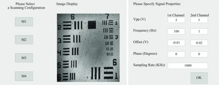
The operation of the overall microscopy system is controlled by software running on a computer connected to a DAQ card embedded in the system. The DAQ card is utilized to generate actuation signals that are applied to the laser steering device and acquire individual pixel intensity values to construct a meaningful image on the screen. In order to control the system via the DAQ card, a MATLAB code is implemented. The user can alter certain properties of the scanning operation by setting related parameters on the designed GUI shown in Figure 3.

Figure 3. GUI of the proposed microscopy system software: the main window where M1, M2, M3, and M4 buttons denote four scanning modes of the system and signal properties window for mode 2 .

at the beginning according to the stated signal specifications, and then the image acquisition process begins. The aforementioned four scanning modes are available on the GUI and the user can choose one desired mode depending on the application. After selecting a scanning mode option, the signal properties screen (SPS), which is shown in Figure3, appears on the screen. From the SPS, properties of actuation signals such as amplitude, frequency, offset, phase, and sampling rate can be adjusted. For options with raster scanning, waveforms of actuation signals are sawtooth and two separate output channels of the DAQ card are utilized. On the other hand, for options with Lissajous scanning, the actuation signal is composed of two sinusoidal signals. Therefore, it is sufficient to employ just one output channel of the DAQ card in the process. The actuation signals are created in MATLAB as a matrix by using built-in MATLAB commands. Sampling rates up to 3 MHz can be used to generate signals. The matrix is transmitted to the DAQ card’s output by using commands again in MATLAB.

The image acquisition part follows the signal generation part. As the first step, voltage values are transformed from the output current value of the PMT by a resistor. Then the voltage values are gathered by the DAQ card in a serial manner through a single analog input channel. To designate the pixel value of the gathered voltage values, a gray-level mapping method is applied. The voltage value, Vpixel, is mapped to a value between 0 and 255 in the mapping process, where 0 value represents black and 255 represents white color. After the mapping process, the acquired pixel’s position in the final image is determined depending on the selected scanning option. When the image acquisition process is accomplished, the final image is successfully displayed on the GUI.

3.1. Raster scanning

In real-time image acquisition process, the DAQ card generates an actuation signal for one period of slow scan axis actuation signal. This is the time for scanning the entire target only once. This can be stated as:

tacq= 1

fslow

, (1)

where tacqis image acquisition time and fslow is slow scan frequency. The number of rows and number of pixels in a row (number of columns) of the constructed image depend on fast scan frequency, slow scan frequency, and

sampling rate:

Nrows=

ffast

fslow

, (2)

where Nrows represents the number of rows of the resulting image, ffast is fast scan frequency, and fslow is slow scan frequency. The ratio between fast and slow scan frequencies is decisive for the number of rows of the constructed image.

Npixels=

fstacq

Nrows

, (3)

where Npixels is number of pixels in a row, fs stands for sampling rate, tacq represents image acquisition time, and Nrows symbolizes number of rows. However, because of barrel distortion, pixels at the edge are not smooth. Therefore, the resulting image is cropped nearly 7.5% from left and right side, i.e. assume that the galvanometric scan mirror’s slow scan frequency is equal to 1 Hz, fast scan frequency to 100 Hz, and sampling rate to 20 kHz. In this situation, the image acquisition time is 1 s for an image. Number of rows is 100 and number of pixels in a row is 200. As a consequence of barrel distortion, the resulting image is cropped from 7.5% from the left and right side. In the end, a 170 × 100 image is displayed on the GUI for this scenario.

For the real-time display, one period of the scanning process is repeated until the user decides to stop the process. To decide the frame per second (FPS) value of the system, Eq. (4) can be used:

F P S = 1

tacq+ top

, (4)

where tacq is image acquisition time in Eq. (1) and top is the process time of the MATLAB code. Nominal values for tacq and top are experimentally acquired as 1.17 s and 0.81 s, respectively. Total image display time ( tacq+ top) can be computed as 1.98 s. Thus, the FPS value of the system is 0.505.

3.2. Lissajous scanning

In the proposed LSCM system, a 3D printed polymer scanner is utilized as a scanning unit and compared with the conventional galvanometric scan mirrors. Lissajous scanning is preferred because in raster scanning the resolution of acquired images depends on the proportion of fast and slow scan frequencies, and for polymer scanners, the ratio between fast and slow scan frequencies could be very low. Therefore, acquiring a meaningful image may not be possible. However, raster scanning with scanner option (mode 4) is available in GUI in the case of usage of a suitable scanning device whose fast and slow scan frequencies are appropriate. Lissajous scanning patterns are often employed in laser scanning systems where the more common raster scanning pattern is impractical. This is often the case in miniaturized laser scanning microscopes using MEMS scanning mirrors or piezoelectric fiber scanners for beam scanning [18,20,22,31–33] since, with appropriate scanning frequencies, the desired FOV can be scanned completely by Lissajous patterns. Usage of Lissajous scanning has led to rapid imaging in atomic force microscopy and multiphoton microscopy [29,31]. It is also reported that, coupled with image interpolation algorithms, 2D Lissajous scanning provides frame rates above 1 kHz [34,35].

Mathematically speaking, a Lissajous curve is the graph of a system of parametric Eqs. (5) and (6):

x(t) = X sin(2πfxt + ϕx), (5)

which describe complex harmonic motion. Here fx and fy are actuation frequencies in the x and y directions while ϕx and ϕy are phase shifts. X and Y are the maximum values x(t) and y(t) could reach. In other words,

X and Y represent borders for the field of view (FOV) in the x and y directions, respectively. The image

constructed from these equations is highly sensitive to the ratio fx/fy. The number of lobes for the targeted figure is also determined by the ratio. For example, a ratio of 2/1 produces a figure with two major lobes. In the same manner, a ratio of 4/3 creates a figure with four horizontal lobes and three vertical lobes.

While constructing an image from data collected by Lissajous scanning, the points resulting from Eqs. (5) and (6) are used as pixel locations. Each data point must be placed in the corresponding (y(tn), x(tn)) position in the image matrix. Here, y(tn) and x(tn) are row and column number for nth data, respectively. However, it is known that row and column numbers of a matrix must be positive integers. To ensure this condition, a series of processes must be applied to Eqs. (5) and (6).

First of all, Eqs. (5) and (6) must be transformed to:

x(t) = 1

2X[sin(2πfxt + ϕx) + 1], (7)

y(t) =1

2Y [sin(2πfyt + ϕy) + 1]. (8)

As a result of Eqs. (7) and (8), x(t) and y(t) values become such that 0⩽ x(t) ⩽ X , 0 ⩽ y(t) ⩽ Y .

Resolution of the constructed image depends on the numerical aperture (NA) of the objective lens and wavelength of the utilized laser in the system. Width and height of the constructed image must be scaled according to the lateral full-width-half-maximum (FWHM) resolution value, which can be expressed as [35]:

wr=2

√

ln 2 0.32 λ

N A , (9)

where N A is the numerical aperture of the lens and λ is the wavelength of the utilized laser. To specify the width and height of the image, X and Y values are divided with the lateral FWHM resolution wr. Image

width and image height can be expressed as:

Iw= X wr , (10) Ih= Y wr , (11)

where Iw and Ih represent image width and height, respectively. To assign position data x(t) and y(t) values between 0 and Iw or Ih, they are also divided with the lateral FWHM resolution wr:

x(t)s= x(t) wr , (12) y(t)s= y(t) wr , (13)

where x(t)s and y(t)s are scaled versions of x(t) and y(t) , respectively. As a result of the process x(t)s and

of that, to eliminate all zero values in x(t)s and y(t)s, 1 is added to them and then they are rounded because x(t)s and y(t)s are used as matrix indexes and therefore they must be positive integers.

Elements of scanning data are placed in the matrix according to corresponding row and column index values x(t)s and y(t)s. In the end, the image is constructed. However, in image acquisition with a DAQ

card and MATLAB, there is delay between actual scanning data and acquired PMT data. When a session is started on the DAQ card, the DAQ card starts generating driving signals and acquiring values from PMT. However, values generated by PMT are not the actual scanning data until the scanning unit of LSCM starts moving. Therefore, some PMT data at the beginning of the process do not contain any information for image construction. These data points, which are acquired at the beginning of the process, are not employed in the image reconstruction process. In the experiments, it has been found that the unused data points correspond to 0.01% of the total acquired data points.

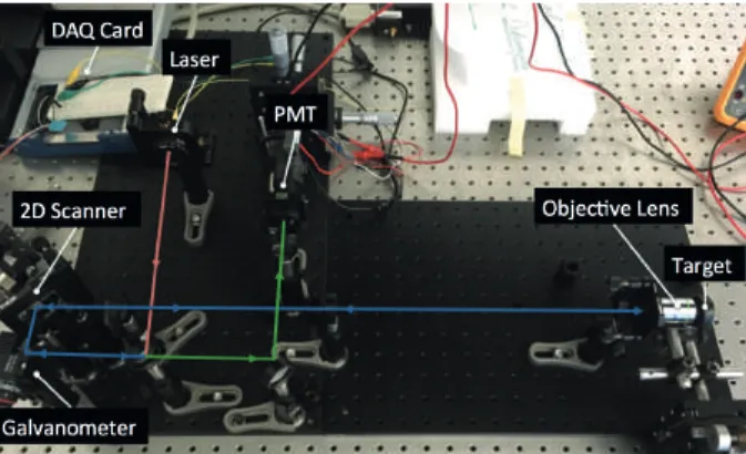
Figure 4. Implemented table-top laser scanning confocal microscopy system. System incorporates a 3D printed 2D polymer scanner and a conventional off-the-shelf 2D galvanometric scan mirror on the same optical path.

4. Experimental results and discussion

The test setup, which is composed of a Thorlabs-LP660-SF60 60 mW laser source with a wavelength of 658 nm, optical lenses, a Hamamatsu-H10721-20 photo-multiplier tube, an NI-USB 6356 data acquisition card, a 2D polymer scanner, and a Thorlabs-GVS002 2D galvanometer scan mirror system that works as the basic scanning unit, is displayed in Figure4. In the conducted tests of the system, it has been observed that lateral resolution of images acquired by utilizing the galvanometric scan mirror can be under 1 µm both in the horizontal and the vertical axis. The values can be adjusted according to the desired resolution and FOV. While horizontal resolution depends on the sampling rate of the DAQ card, vertical resolution depends on ratio between fast and slow scan frequencies and the ratio depends on specifications of the scanning unit as explained in Section 3. FOV, FPS, and lateral resolution values for the galvanometric scan mirror and polymer scanner under a Lissajous scanning scheme are tabulated in the Table. As summarized in the Table, compared to conventionally preferred off-the-shelf galvanometric scan mirrors, the polymer scanner has a lower lateral resolution, much smaller FOV, and equivalent FPS.

Table. FOV, FPS, and lateral resolution values for galvanometric scan mirror and polymer scanner using a Lissajous scanning scheme.

Scanning unit FOV Lateral resolution FPS

Galvanometric scan mirror 420 µm× 360 µm 1 µm 0.4 Polymer scanner 117 µm× 117 µm 3.2 µm 0.5

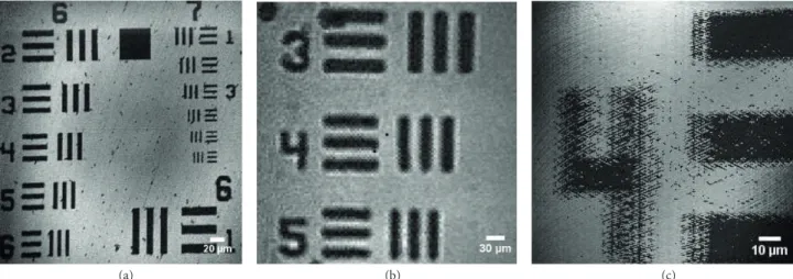
As the first step, the system has been optically characterized by imaging the USAF 1951 resolution target by employing mode 1, mode 2 and mode 3 . Resulting images are shared in Figure 5. As can be clearly seen from the figures, the off-the-shelf 2D galvanometric scan mirror optically outperforms the polymer-scan mirror considering Figures 5a and 5b, which are acquired using the galvanometer, and Figure 5c, which is obtained using the polymer scanner incorporated in the system. In mode 2, due to the finer resolution provided by the

(a) (b) (c)

Figure 5. USAF 1951 resolution target images obtained by using different scanning modes of the system. Images are obtained with (a) mode 2 ( fs = 1 MHz, fslow= 1 Hz, and ff ast= 100 Hz); (b) mode 1 ( fs = 100 kHz, fx= 101 Hz, and fy= 100 Hz); and (c) mode 3 ( fs = 100 kHz, fslow= 117 Hz, and ff ast= 262 Hz) scanning modes of the system, respectively.

raster-scanning, Figure5a is acquired from a smaller area, groups 6 and 7 of the USAF 1951 resolution target. On the other hand, since Lissajous scanning in mode 1 provides a coarser resolution compared to raster scanning in mode 2 , Figure5b covers a larger area, group 4 of the same target. Figure5c is acquired by utilizing mode 3 of the system. Since coarser resolution and lower FOV values are provided in mode 3 due to the polymer scanner integrated in the system, the image is scanned from a part of group 4 of the resolution target to compare with the other modes.

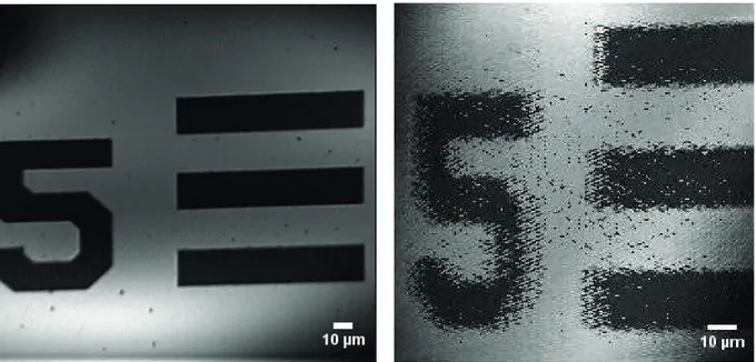
Moreover, in Figure6, a very clear comparison between LSCM images obtained by employing mode 1 and mode 3 from the same location on the USAF 1951 resolution target is shown. It can be said without any reservation that the images acquired from exactly the same location and with precisely the same optical equipment prove that the market-available off-the-shelf galvanometric scan mirror optically outperforms the polymer scanner by far. However, for cheaper portable scanning microscopy devices, polymer scanners can still be considered in systems for initial diagnosis with 3.2 µ m lateral resolution.

The implemented microscopy system is also clinically tested on various biological samples such as bacterial cells (yeast) and red blood cells in order to see and measure its optical performance. Resulting images are shared in Figure7. In Figure7a, red blood cells are clearly distinguishable, whereas in Figure7b, a detailed image of bacteria cells (yeast) under our proposed LSCM system can be easily seen. Each bacterial cell has a size of nearly 2 µm and is clearly distinguishable.

5. Conclusion

In this paper, we have developed a laser scanning confocal microscopy system to utilize combinations of various scanning devices and methods and to be able to characterize the optical performance of different scanners and micromirrors that are frequently used in scanning microscopy systems such as multiphoton microscopy, optical

(a) (b)

Figure 6. Resolution target images from the same image frame obtained by using different scanning units: (a) acquired with mode 2 ( fslow= 1 Hz and ff ast= 100 Hz), (b) with mode 3 ( fslow = 117 Hz and ff ast= 262 Hz).

(a) (b)

Figure 7. Scanning results of various specimens with mode 2 scanning mode of the system: (a) red blood cells ( fslow= 0.1 Hz and ff ast= 100 Hz), (b) bacterial cells ( fslow= 0.1 Hz and ff ast= 100 Hz).

coherence tomography, or confocal microscopy. By simply integrating the MEMS scanner to be benchmarked on the same optical path of a commercially available off-the-shelf galvanometric scan mirror, we aimed to automatically get microscopy images from the same location on the target specimen without having any time-consuming alignment problems. By taking various images from both the resolution target and biological specimen, we experimentally showed that this novel optical configuration provided a high-quality optical comparison opportunity between the laser scanning devices. Moreover, we proved our claim that this new optical setup eliminates the utilization of a second scanning microscopy to benchmark the performance of the scanner-based system and considerably reduces the time spent for imaging, which is a crucial factor for freshly excised tissue, especially under a fluorescence microscope.

In the above discussion, we showed that the off-the-shelf 2D galvanometric scan mirror outperforms by far the polymer scanners that are used in our proposed optical configuration. Attained FPS, FOV, and lateral resolution values are tabulated in the Table. However, even though the optical performance of scanner is lower, it can be still preferred especially in portable laser scanning microscopy systems thanks to the small size and weight compared to motorized, bulky, and expensive galvanometer systems.

Acknowledgment

The authors would like to thank TÜBİTAK SBAG for funding this project with research grant number 113S114. References

[1] Guyon I, Elisseeff A. An introduction to variable and feature selection. J Mach Learn Res 2003; 3: 1157-1182. [2] Izadpanahi S, Özçınar Ç, Anbarjafari G, Demirel H. Resolution enhancement of video sequences by using discrete

wavelet transform and illumination compensation. Turk J Elec Eng & Comp Sci 2012; 20: 1268-1276. [3] Haupt RL, Haupt SE. Practical Genetic Algorithms. 2nd ed. New York, NY, USA: Wiley, 2004. [4] Kennedy J, Eberhart R. Swarm Intelligence. San Diego, CA, USA: Academic Press, 2001.

[5] Poore JH, Lin L, Eschbach R, Bauer T. Automated statistical testing for embedded systems. In: Zander J, Schieferdecker I, Mosterman PJ, editors. Model-Based Testing for Embedded Systems. Boca Raton, FL, USA: CRC Press, 2012. pp. 111-146.

[6] Li RTH, Chung SH. Digital boundary controller for single-phase grid-connected CSI. In: IEEE 2008 Power Elec-tronics Specialists Conference; 15–19 June 2008; Rhodes, Greece. New York, NY, USA: IEEE. pp. 4562-4568. [7] Boynukalın Z. Emotion analysis of Turkish texts by using machine learning methods. MSc, Middle East Technical

University, Ankara, Turkey, 2012.

[8] Sheppard CJR, Shotton D. Confocal Laser Scanning Microscopy. 1st ed. New York, NY, USA: Garland Science, 1997.

[9] Einstein AJ. Medical imaging: the radiation issue. Nat Rev Cardiol 2009; 6: 436.

[10] Lundstedt C, Stridbeck H, Andersson R, Tranberg KG, Andrén-Sandberg A. Tumor seeding occurring after fine-needle biopsy of abdominal malignancies. Acta Radiol 1991; 32: 518-520.

[11] Li G, Li H, Duan X, Zhou Q, Zhou J, Oldham KR, Wang TD. Visualizing epithelial expression in vertical and horizontal planes with dual axes confocal endomicrosope using compact distal scanner. IEEE T Med Imaging 2017; 36: 1482-198.

[12] Dixon AE, Damaskinos S, Atkinson MR. A scanning confocal microscope for transmission and reflection imaging. Nature 1991; 351: 551-553.

[13] Wilson T. Confocal Microscopy. San Diego, CA, USA: Academic Press, 1990. [14] Paddock SW. Confocal laser scanning microscopy. Biotechniques 1999; 27: 992-1004.

[15] Mowla A, Taimre T, Bertling K, Wilson S, Rakic A. Confocal laser feedback microscopy for in-depth imaging applications. Electron Lett 2018; 54: 196-198.

[16] Mowla A, Taimre T, Lim YL, Bertling K, Wilson SJ, Prow TW, Rakic AD. A compact laser imaging system for concurrent reflectance confocal microscopy and laser Doppler flowmetry. IEEE Photonics J 2016; 8: 1-9.

[17] Kumar K, Avritscher R, Wang Y, Lane N, C Mado DC, Yu TK, Uhr JW, Zhang X. Handheld histology-equivalent sectioning laser-scanning confocal optical microscope for interventional imaging. Biomed Microdevices 2010; 12: 223-233.

[19] Gruber A, Drabenstedt A, Tietz C, Fleury L, Wrachtrup J, Von Borczyskowski C. Scanning confocal optical microscopy and magnetic resonance on single defect centers. Science 1997; 276: 2012-2014.

[20] Hoy CL, Durr NJ, Ben-Yakar A. Fast-updating and nonrepeating Lissajous image reconstruction method for capturing increased dynamic information. Appl Optics 2011; 50: 2376-2382.

[21] Hung ACL, Lai HYH, Lin TW, Fu SG, Lu MSC. An electrostatically driven 2D micro-scanning mirror with capacitive sensing for projection display. Sensor Actuat A-Phys 2015; 222: 122-129.

[22] Helmchen F, Denk W, Kerr JND. Miniaturization of two-photon microscopy for imaging in freely moving animals. Cold Spring Harbor Protocols 2013; 2013: pdb-top078147.

[23] Qiu Z, Rhee CH, Choi J, Wang TD, Oldham KR. Large stroke vertical PZT microactuator with high-speed rotational scanning. IEEE J Microelectromech Syst 2014; 23: 256-258.

[24] Erden MS, Rosa B, Boularot N, Gayet B, Morel G, Szewczyk J. Conic-Spiraleur: A miniature distal scanner for confocal microlaparoscope. IEEE ASME T Mechatron 2014; 19: 1789-1798.

[25] Urey H. Torsional MEMS scanner design for high-resolution scanning display systems. In: Optical Scanning; 2002; Seattle, WA, USA. Bellingham, WA, USA: International Society for Optics and Photonics. pp. 27-38.

[26] Wang Y, Gokdel YD, Triesault N, Wang L, Huang YY, Zhang X. Magnetic-actuated stainless steel scanner for two-photon hyperspectral fluorescence microscope. IEEE J Microelectromech Syst 2014; 23: 1208-1218.

[27] Yalcinkaya AD, Urey H, Brown D, Montague T, Sprague R. Two-axis electromagnetic microscanner for high resolution displays. J Microelectromech S 2006; 15: 786-794.

[28] Oyman HA, Gokdel YD, Ferhanoglu O, Yalcinkaya AD. Performance of a three-dimensional-printed microscanner in a laser scanning microscopy application. Opt Eng 2018; 57: 57-64.

[29] Bazaei A, Yong YK, Moheimani SOR. High-speed Lissajous-scan atomic force microscopy: Scan pattern planning and control design issues. Rev Sci Instrum 2012; 83: 063701.

[30] Hoy CL, Durr NJ, Ben-Yakar A. Fast-updating and nonrepeating Lissajous image reconstruction method for capturing increased dynamic information. Appl Optics 2011; 50: 2376-2382.

[31] Flusberg BA, Jung JC, Cocker ED, Anderson EP, Schnitzer MJ. In vivo brain imaging using a portable 3.9? gram two-photon fluorescence microendoscope. Opt Lett 2005; 30: 2272-2274.

[32] Hoy CL, Durr NJ, Chen P, Piyawattanametha W, Ra H, Solgaard O, Ben-Yakar A. Miniaturized probe for femtosecond laser microsurgery and two-photon imaging. Opt Express 2008; 16: 9996-10005.

[33] Liu TM, Chan MC, Chen IH, Chia SH, Sun CK. Miniaturized multiphoton microscope with a 24Hz frame-rate. Opt Express 2008; 16: 10501-10506.

[34] Tuma T, Lygeros J, Kartik V, Sebastian A, Pantazi A. High-speed multiresolution scanning probe microscopy based on Lissajous scan trajectories. Nanotechnology 2012; 23: 185501.

[35] Zipfel WR, Williams RM, Webb WW. Nonlinear magic: multiphoton microscopy in the biosciences. Nat Biotechnol 2003; 21: 1369-1377.