Clustering protein-protein interactions based on conversed domain similarities

CLUSTERING PROTEIN-PROTEIN

INTERACTIONS BASED ON CONSERVED

DOMAIN SIMILARITIES

A THESIS

SUBMITTED TO THE DEPARTMENT OF COMPUTER ENGINEERING AND THE INSTITUTE OF ENGINEERING AND SCIENCE

OF BILKENT UNIVERSITY

IN PARTIAL FULFILLMENT OF THE REQUIREMENTS FOR THE DEGREE OF

MASTER OF SCIENCE

By

Aslı Ayaz

August, 2004

ii I certify that I have read this thesis and that in my opinion it is fully adequate,

in scope and in quality, as a thesis for the degree of Master of Science. ____________________________________

Assist. Prof. Dr. Uğur Doğrusöz (Supervisor)

I certify that I have read this thesis and that in my opinion it is fully adequate, in scope and in quality, as a thesis for the degree of Master of Science.

____________________________________ Prof. Dr. Özgür Ulusoy

I certify that I have read this thesis and that in my opinion it is fully adequate, in scope and in quality, as a thesis for the degree of Master of Science.

____________________________________ Assist. Prof. Dr. Uygar Tazebay

Approved for the Institute of Engineering and Science:

_____________________________________ Prof. Dr. Mehmet B. Baray

iii

ABSTRACT

CLUSTERING PROTEIN-PROTEIN INTERACTIONS

BASED ON CONSERVED DOMAIN SIMILARITIES

Aslı Ayaz

M.S. in Computer Engineering

Supervisor: Assist. Prof. Dr. Uğur Doğrusöz

August, 2004

Protein interactions govern most cellular processes, including signal transduction, transcriptional regulation and metabolism. Saccharomyces ceravisae is estimated to have 16,000 protein interactions. Appereantly only a small number of these interactions were formed ab initio (invention), rest of them were formed through gene duplications and exon shuffling (birth). Domains form functional units of a protein and are responsible for most of the interaction births, since they can be recombined and rearranged much more easily compared to innovation. Therefore groups of functionally similar, homologous interactions that evolved through births are expected to have a certain domain signature. Several high throughput techniques can detect interacting protein pairs, resulting in a rapidly growing corpus of protein interactions. Although there are several efforts for computationally integrating this data with literature and other high throughput data such as gene expression, annotation of this corpus is inadaquate for deriving interaction mechanism and outcome. Finding interaction homologies would allow us to annotate an unannotated interaction based on already annotated known interactions, or predict new ones. In this study we propose a probabilistic model for assigning interactions to homologous groups, according to their conserved domain similarities. Based on this model we have developed and implemented an Expectation-Maximization algorithm for finding the most likely grouping of an interaction set. We tested our algorithm with synthetic and real data, and showed that our initial results are very promising. Finally we propose several directions to improve this work.

iv

ÖZET

PROTEİN-PROTEİN ETKİLEŞİMLERİNİN

KORUNMUŞ BÖLGE BENZERLİĞİNE GÖRE

ÖBEKLENMESİ

Aslı Ayaz

Bilgisayar Mühendisligi, Yüksek Lisans

Tez Yöneticisi: Yard. Doç. Dr. Uğur Doğrusöz

Ağustos, 2004

Protein protein etkileşimleri (PPE) sinyal iletimi, transkripsiyonel düzenleme ve metabolizma gibi pek çok hücresel işlemi yürütürler. Saccharomyces ceravisae'de 16,000 civarında PPE olduğu tahmin edilmektedir. Bu etkileşimlerin pek azının rastgele mutasyonlarla evrimleştiği (keşif), diğerlerinin ise gen çiftlenmesi ve exon değişimi gibi olaylarla oluştuğu (doğum) kabul edilmektedir. Bölgeler, proteinlerin işlevsel birimleridir, ve yeniden derlenip düzenlenebildikleri için doğumların çoğundan sorumludurlar. Dolayısıyla doğumlar yoluyla evrimleşmiş eşköklü etkileşimlerin ortak bölgelerden oluşan bir imzası olması beklenir. PPE’leri tespit eden bir kaç yüksek üretimli yöntem sayesinde, hızla artan miktarlarda PPE verisi elde edilmektedir. Bu verileri literatür ve gen ifadesi gibi diğer yüksek verimli verilerle tümleştirmek için çabalar bulunsa da, hali hazırdaki verilerle ilişkilendirilmiş bilgiler etkileşimin mekanizmasını ve işlevini anlamak için yetersizdir. Etkileşim eşköklülüğünün tespiti, yeni ya da bilinmeyen etkileşimlerin, eşköklü bilinen etkileşimler yoluyla tanımlanmasını sağlayabilir. Bu çalışmada bölge benzerliğini esas alarak etkileşimleri eşköklü gruplara atamak için olasılıksal bir model tanımlıyoruz. Bu modeli temel alarak, en olası öbeklemeyi bulmak için bir Beklenti-Maksimizasyon algoritması geliştirdik. Algoritmayı sentetik ve gerçek veriler üzerinde sınadık ve ilk sonuçların oldukça umut verici olduğunu gösterdik. Son olarak bu çalışmanın geliştirilebilmesi için bir kaç öneri sunduk.

v

Acknowledgement

I would like to express my gratitude to my supervisor Assist. Prof. Uğur Doğrusöz, for his guidance, valuable comments and incredible effort in the writing of this thesis. I learned many things from him not only during the thesis process but also in the development of our team project, PATIKA. It was a great pleasure and chance for me to work with him.

I would like to thank Prof. Özgür Ulusoy and Assist. Prof. Uygar Tazebay for reviewing the manuscript of this thesis.

I wish to thank Özgün Babur for his patience during our weekly meetings and his critical comments. I also wish to thank Ozan Gerdaneri, Zeynep Erson, Erhan Giral, and all other members of the PATIKA team. It was a great experience to be a member of such a friendly team. They have been another family for me.

It is not possible to thank Emek Demir enough. Without his support and contributions this thesis would not be possible. He was very patient during our endless discussions on the model and came up with bright ideas. He has always encouraged and guided me when I felt totally lost and thought it was impossible. This world is more beautiful with him.

Above all, I am very grateful for the love and support of my parents Nevin and Servet, and my sister Ödül. In every step of my life there is their love and trust.

vi

Contents

Chapter 1 Introduction ...1

Chapter 2 Theory and Background ...4

2.1 Basics ...4

2.2 Protein Interactions...6

2.2.1 Yeast Two-Hybrid ...7

2.2.2 Mass Spectrometry ...9

2.2.3 X-ray Crystallography ...10

2.2.4 Protein Interaction Databases ...10

2.3 Properties of Proteins ...11

2.3.1 Domains...12

2.3.2 GO Annotations...14

2.3.3 Swiss-Prot Keywords...15

Chapter 3 Related Work ...16

3.1 Protein Function Prediction...16

3.2 Properties of a PPI Network ...17

3.3 PPI Inference ...18

3.4 Domain Interaction Inference ...18

Chapter 4 Method...20 4.1 Problem Definition...20 4.2 Clustering Approach ...22 4.2.1 Probabilistic Model...23 4.2.2 EM Algorithm...25 4.3 Complexity Analysis ...27 Chapter 5 Results...30 5.1 Hypothetic Data ...30

vii 5.2 Real Data ...31 5.3 Clustering Evaluation ...32 5.3.1 Statistical Entropy...32 5.3.2 Probabilistic Entropy ...33 5.3.3 Unsupervised Entropy ...33

5.4 Hypothetic Data Results...34

5.5 Real Data Results ...39

5.5.1 Clustering of Real Sample Data...39

5.5.2 Clustering of Entire Data Set ...43

Chapter 6 Implementation ...45

6.1 PATIKA ...45

6.2 Bioentity Graphs ...46

Chapter 7 Conclusion and Discussion...49

References ...52

Appendix A Hypothetic Data Clustering...58

A.1 Example 1...58

viii

List of Figures

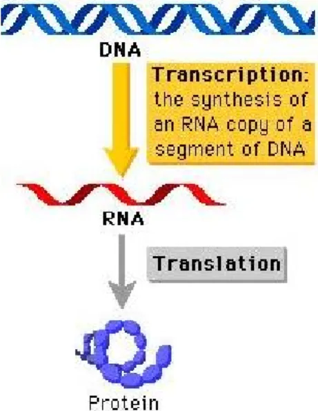
Figure 1: Central Dogma. RNA is synthesized from DNA by a process called transcription and protein is

synthesized from RNA segment by a process called translation. ...5

Figure 2: PPI map of 1870 proteins of yeast [7]. Each circle represents a different protein and each line indicates that the two end proteins are capable of binding to one another. The colour of a node represents the phenotypic effect of removing the corresponding protein (red: lethal, green: non-lethal, orange: slow growth, yellow: unknown). ...7

Figure 3: Regulation of gene expression in yeast...8

Figure 4: Y2H assay (modified from [9]) ...9

Figure 5: Crystal structure of one of the four subunits of pyruvate kinase [26]...13

Figure 6: GO terms associated with tumor suppressor protein p53 ...14

Figure 7: Swiss-Prot keyword annotation of p53 protein...15

Figure 8: Domains of ERBB2 according to Pfam. ...21

Figure 9: Cluster distribution of hypothetic data of 400 symmetric interactions (A-B and B-A) of 1000 proteins. Each protein is defined by 500 features. Interactions are created according to 20 cluster rules without introducing any error to the rules. This figure represents cluster distributions of clusters obtained by EM. Each bar represents percentage of members coming from hypothetic clusters and colors represent hypothetic clusters. Color hypothetic cluster mapping is given with the legend on the right. ...35

Figure 10: Cluster distributions of sample real data of 188 interactions...41

Figure 11: Basics of state-transition level ontology...45

Figure 12: Different type of bioentities and bioentity interactions types of PATIKA. Nodes correspond to bioentities and the edges correspond to bioentity interactions...47

Figure 13: Bioentity graph of sample real PPI data with their assigned clusters. Different colors represent different clusters. ...48

Figure 14: Cluster distributions...59

ix

List of Tables

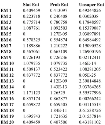
Table 1: Total entropy values calculated for each run of the algorithm. Total statistical entropy and total probabilistic entropy show similar pattern, whereas the unsupervised entropy behaves differently.

According to first two entropy measures 10th _{run gives the best clustering. ...34}

Table 2: Entropy measures. Three different entropy measures of each clusters obtained at the 10th _{run of the} clustering algorithm. Statistical entropy values and probabilistic entropies give similar results. Cluster 5, 13, 14, 18 have the lowest entropy values according to first two measures...36

Table 3 Distributions of members of clusters. Each row corresponds to one of the resulting clusters of EM algorithm and each column corresponds to one hypothetic cluster. In a row how many members of a cluster originates from each hypothetic cluster can be observed. Last row demonstrates sizes of hypothetic clusters and the last column demonstrates sizes of EM clusters. ...37

Table 4: Matching cluster rules of hypothetic and EM clusters. Yellow regions represent protein-A related part of the rule, blue regions represent protein-B part of an interaction. All hypothetic rule weights are ‘1’ because we did not introduce error to this data set. 18 of the 20 cluster rules could be determined with very high weight values. ...38

Table 5: Cluster rules and sizes of real sample data. First seven rules are forward rules and the remaining rules are obtained by reversing the first seven rules. Protein-A part of the rules are yellow and the protein-B parts are blue. ...40

Table 6: Cluster member distributions of sample real data clustering. Rows correspond to clusters obtained as result of EM clustering and columns correspond to real clusters. ...41

Table 7: Rules of clusters obtained by EM. ...43

Table 8: Some interaction cluster rules obtained as a result of entire real data set clustering...44

Table 9: Total entropies for each run. 9th _{run has the lowest entropy. ...59}

Table 10: Entropy measures of clusters. ...60

Table 11: Distributions of members of clusters. ...61

Table 12: Matching hypothetic and EM cluster rules. ...62

Table 13: Total entropies ...63

Table 14: Entropy values of each cluster of run 3...63

Table 15: Distributions of members of clusters. ...65

1

Chapter 1 Introduction

Life is a very complex mechanism and requires a strict regulation and synchronization of inter and intra-cellular processes. Every second, a cell must respond to a plethora of inputs, changing its internal state, activating proper processes and give back an appropriate output when necessary. All these processes and regulations are mediated by the interactions of molecules [1].

Proteins, with their sheer numbers and functional variety, are responsible for most of these tasks. From metabolic enzymes to receptors to transcription factors, they facilitate chemical reactions, create complex decision making mechanisms and transduce signals by regulating each other. Mutations that result in aberrant, malfunctioning proteins are responsible for most of the hereditary diseases and cancer. One of the most important goals of the proteomics era is to reveal and understand the complex network of protein-protein interactions (PPIs). Although the problem has multiple aspects, it can be roughly expressed in terms of four important questions: “What interacts with what?”, “under which conditions?”, “what is the mechanism of interaction?” and “what is the outcome?”

There are several challenges for this task. Perhaps the most important challenge, which is only recently being acknowledged by the scientific community, is the need for systems level analysis and modeling. It has been shown that like many other social and biological networks, PPI networks are small-world graphs, which implies that although it is possible to identify modules that act together, modules themselves are also highly coupled with each other. Therefore analysis of the functions of isolated proteins or even modules is limited to partial if not erroneous results. Another important challenge comes from the transient nature of protein-protein interactions. Two proteins might be interacting briefly, under a very specific condition making the interaction hard to detect,

2 and even harder to observe its mechanism and outcome. This has not been the case with genetic or protein structure studies, which concern most of the time relatively static and stable mechanisms.

Finding interacting pair of proteins is the most straightforward subproblem and is already being addressed by various experimental studies, including cross-linking, fluorescence energy transfer analysis, protease digestion and western blotting. More importantly, new high throughput techniques such as yeast two-hybrid and phage display allowed researchers to produce organism-wide interaction maps in the last several years. However one should always bear in mind that these techniques also produce a substantial amount of false positives and negatives compared with conventional techniques. There are ongoing efforts to increase reliability of these methods, and to complement them with other techniques to identify errors.

Despite of recent advances in fluorescence resonance energy transfer, X-ray crystallography, mass spectrometry and other state-of-the-art techniques, there is still no high throughput technique for identifying conditions and mechanisms of PPIs. This makes computational methods even more important. Integrating data on existing knowledge bases, computational biologists infer, model and test in silico systems, hopefully developing useful explanations on how complex biological systems operate.

Research shows that for eukaryotes, only a very small fraction of PPIs evolved ab initio [2]. Rest of them evolved through gene duplications and exon shuffling, reusing existing functional domains in the proteins over and over. The modularity of the domains allows rapid evolution of molecular networks. An example is SH2 domain [3], which is missing in yeast, but is present and widespread in every multicellular organism. Therefore SH2 must have been originated in one of the first multicellular organisms, possibly along with protein tyrosine kinases which are also missing in yeast. However SH3 domain is present in 28 yeast proteins, which also have human homologs. 11 of these homologs also contain SH2 domains, indicating that these proteins acquired the needed function instead of inventing them [4].

This idea points us to a notion of interaction homology and families, similar to gene families. Protein pairs interacting over homologous functional domains should be similar in function and mechanism. Finding these families would be of immense benefit, since it

3 would make computational annotation of a whole family possible once a member of the family is annotated. Similarly finding such families across different organisms would be very valuable for comparative proteomics.

In this study we aim to find such homologous interaction groupings. Using the domain information of the interacting pairs, we try to determine a set of clusters of interactions such that all interactions in a certain cluster has a common subset of domains, and overlaps between these clusters are minimal. We have developed a probabilistic model and used an Expectation-Maximization algorithm to find most likely clustering. Once such clusters are obtained they can be used for annotating protein interaction data.

4

Chapter 2 Theory and Background

2.1

Basics

Every cell in an organism is assumed to have a complete copy of the genome, specific to that organism. Large chains of DNA molecules form the genome, which can be modeled as strings of a four letter alphabet with A, T, C and G corresponding to different types of nucleotides. Each chain forms a helix with its complementary chain.

DNA encodes most of the functionality and the structure that forms the organism. This code is first converted to RNA molecules and then to protein molecules which are the usual executers of the code. Transmission of the code from DNA to RNA molecules is called transcription and interpretation of this code from RNA to protein is called translation. As a whole, this information flow is called the “Central Dogma”.

5

Figure 1: Central Dogma. RNA is synthesized from DNA by a process called transcription and protein is synthesized from RNA segment by a process called translation.

A protein is a macromolecule composed of one or more amino acid chains of specific order. Sequence information is transmitted from the DNA to the RNA and then to the proteins. Proteins are synthesized according to the nucleotide sequences of the gene coding that specific protein. Every triplet of nucleotides encodes one of the 20 amino acids and sequence of these nucleotide triplets determines amino acid order of a protein, which in turn determines the final protein structure.

Proteins have several functions in the cell and they are categorized according to their functions:

− Enzymes catalyze specific reactions via interaction to the reactants and increase the reaction rate. An example is phosphorylation of pyruvate by pyruvate kinase.

− Regulatory proteins regulate the metabolism of the cells. Hormones and transcription factors are some examples of this group of proteins. Hormones such as insulin regulates glucose intake to the cell, whereas transcription factor p53 activates transcription of p21 protein in the presence of DNA damage.

6 − Transport proteins, either binds to small molecules such as O2 or fatty

acids and carries them in the blood or they may help transport of molecules through the membranes. (e.g. glucose transporter).

− Storage proteins act as reservoirs of nutrients. Some examples are casein in milk as amino acid storage and ferritin as iron storage.

− Contractile and motile proteins, function in the movement of cells, or movement in a cell. For example actin and myosin allows muscle contractions whereas tubulin functions in the mitotic spindle formation.

− Structural proteins help the formation of the structure of the cell or the tissues. Cytoskeletal proteins form the cellular structure.

− Protective proteins such as immunoglobulins or antibodies function in the immune response.

Proteins might have multiple functions. Their globular structure, composition of multiple globular domains, allows them to perform different functions.

2.2

Protein Interactions

All the above functions are carried out by interactions of proteins with other molecules such as small molecules, nucleic acids and other proteins. In the last few years, genetic information accumulated in an exponential rate and genomes of many organisms have been sequenced. However the knowledge of expressed genes and their sequence do not tell us a lot about the mechanism of biological processes. Comprehensive information on protein interactions would be valuable in understanding of the cellular program. Among these interactions protein-protein interactions (PPIs) are fundamental to cellular processes. They are responsible for critical processes such as metabolism, replication, transcription and most of the regulatory events. An organism contains PPIs in the order of ten thousands related with the size of its genome. For example it is estimated that there are about five interaction partners per protein in yeast when the most highly connected proteins are

7 excluded and eight partners otherwise [5]. This estimate suggests 16,000 – 26,000 interaction pairs in yeast.

Conventionally PPIs are detected via various experimental techniques such as western blotting, cross-linking and protease digestion. Recent high-throughput experimental techniques such as Yeast Two-Hybrid (Y2H) or Mass Spectrometry (MS) allowed scientific community to produce large amounts of PPI data (Figure 2).

Figure 2: PPI map of 1870 proteins of yeast [6]. Each circle represents a different protein and each line indicates that the two end proteins are capable of binding to one another.

2.2.1 Yeast Two-Hybrid

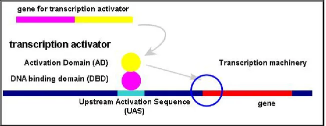
Yeast two-hybrid (Y2H) [7]is a genetic assay to detect PPIs. This assay makes use of the process of regulation of gene expression in yeast. To activate expression of

8 a gene, a transcription activator protein is required to bind Upstream Activation Sequence (UAS) of a gene. That transcription activator protein has two domains with different functions. One is DNA binding domain (DBD) and the other is activation domain (AD). DBD of transcription activator binds to UAS and AD activates the expression afterwards (Figure 3).

Figure 3: Regulation of gene expression in yeast.

In Y2H assay, artificial gene constructs are prepared to understand whether two proteins X and Y interact. First, the expressed gene is replaced by a reporter gene such as a fluorescent protein to observe the presence of gene expression easily. Then artificial constructs of two-hybrid proteins are prepared (X-DBD and Y-AD). If X and Y proteins interacts, DBD and AD will function properly and activate expression of the reporter gene; otherwise there will be no expression (Figure 4).

9

Figure 4: Y2H assay (modified from [8])

Preparing hybrid proteins associated with DBD and AD of transcription activator in large scales and assaying every pair of proteins in a yeast colony and observation of reporter gene allow us to detect organism wide PPIs.

However one should also bear in mind that Y2Hs are shown to produce a lot of false positives and negatives, due to several reasons including higher-than-normal target concentrations, misfolding due to artificial constructs or inhibitory binding topology. In a recent study [9] it has been shown that phage display and Y2H agree on only 95 out of 551 interactions detected by either one of the system. There are several ongoing efforts to increase reliability of such high throughput methods [10].

2.2.2 Mass Spectrometry

Mass spectrometry, also called mass spectroscopy, is an instrumental approach that allows for the mass measurement of molecules. The five basic parts of any mass spectrometer are: a vacuum system, a sample introduction device, an ionization source, a mass analyzer, and an ion detector. Combining these parts a mass spectrometer determines the molecular weight of chemical compounds by ionizing, separating, and measuring molecular ions according to their mass-to-charge ratio

10 (m/z). The ions are genes. No such message rated in the ionization source by inducing either the loss or the gain of a charge (e.g. electron ejection, protonation, or deprotonation). Once the ions are formed in the gas phase, they can be electrostatically directed into a mass analyzer, separated according to mass and finally detected. The result of ionization, ion separation, and detection is a mass spectrum that can provide molecular weight or even structural information. Traditionally use of MS was limited to analysis of small molecules. However several important advances in the field including Electrospray ionization [11] and soft laser desorption [12] allowed vaporization of large molecules such as proteins and their complexes [13][14][15].

2.2.3 X-ray Crystallography

X-ray crystallography exploits the fact that X-rays are diffracted by crystals [8]. Based on the diffraction pattern obtained from X-ray scattering off the periodic assembly of molecules or atoms in the crystal, the electron density can be reconstructed. A crystal of a protein complex can provide us with the partners of the complex and exact binding geometry. There is a substantial amount of protein complex structures in the Protein Data Bank [16].The problem with X-ray crystallography is to obtain the crystal itself. Although there are several methods for high throughput crystallization, none of them works universally and their data did not appear yet. Besides, transient interactions simply do not live long enough to crystallize and fail to be detected by X-ray crystallography.

2.2.4 Protein Interaction Databases

Data obtained from the above high-throughput techniques led to construction of a number of protein interaction databases.

A.0.1.1 BIND

BIND (Biomolecular Interaction Network Database) [17] has three groups of molecular associations: 1) molecular interactions, 2) molecular complexes and 3) pathways. Interactions are basic units of BIND and these interactions are not only

11 defined between proteins but between biological entities also including DNA, RNA, small molecules, molecular complexes, photons and unidentified entities. Molecular complexes are defined as a collection of two or more molecules to perform a single function. In BIND two or more interactions constitute a molecular complex. Pathways are defined as sequence of two or more interactions. Each BIND entry has to be supported by at least one publication in a peer-reviewed journal. Additional information such as complex topology and number of subunits supports molecular complex entries and pathway entries provides information about in which stage of the cell cycle this pathway is observed and whether this pathway is associated with a specific disease [18].

A.0.1.2 DIP

DIP (Database of Interacting Proteins) [19] stores experimentally determined interactions between proteins. DIP interaction data were curated manually by expert curators and also automatically by a computational approach which utilizes the information about the most reliable core interaction network of DIP [20].

A.0.1.3 MIPS CYGD

CYGD (Comprehensive Yeast Genome Database) contains 15488 annotated PPIs of Saccharomyces cerevisiae, including many high throughput experiment results.[21]

A.0.1.4 IntAct

IntAct [22] is an molecular interactions database that were formed by various European groups including EBI, MINT and SIB and MPI-MG. IntAct currently contains 27652 proteins and 36641 interactions.

2.3

Properties of Proteins

Data available in these databases are pairs of proteins or molecules determined to interact. We will be studying PPIs in this study since they carry out most of the regulatory function and execute the code stored in the genome of the cells. However

12 little or nothing is known about the nature or function of these interactions. But what we know most of the time is the properties of proteins. There are several databases storing available information about the proteins of several organisms. Swiss-Prot [23] is a curated protein sequence database. It provides high level of annotation of proteins such as the description of the function of a protein, its domains structure, post-translational modifications. This database also supports high level of integration with other databases. Protein Information Resource (PIR) supports a similar protein sequence database with high level of annotation [24].

In this study we aim to obtain more information about PPIs by using available data of interacting proteins. For the initial study we restricted our data sets to domain information of proteins, GO annotations and Swiss-Prot keywords.

2.3.1 Domains

Protein domains are structural or functional units of proteins and usually determined by evolutionarily conserved amino acid sequence modules. Proteins interact through their domains so the presence of certain domains in proteins brings the probability of interaction between those proteins. Also functions or structures of domains might provide information about the nature of the interaction. In Figure 5, domain architecture of pyruvate kinase protein can be observed.

13

Figure 5: Crystal structure of one of the four subunits of pyruvate kinase [25].

For example growth factor receptors possess an extracellular domain for capturing the ligand, an intermembrane domain and finally a cytoplasmic protein-tyrosine kinase domain. When the ligand binds to the receptor, receptor forms a dimer through the intermembrane domain, autophosphorylates itself, and finally exposes docking sites for other cytoplasmic signaling proteins. These proteins, although diverse, always contain at least one Src homology 2 (SH2) domains, which is involved in binding to the receptor at specific binding sites. The human genome is estimated to contain 115 proteins containing SH2 domain [3].

SH2 is a prototype for a set of different interaction domains, such as SH3, PDZ, PH, KH or Puf repeat domains. Interaction domains control almost all cellular functions including signal transduction, protein trafficking, gene expression and chromatin organization [4].

In this study we referred to Protein families’ (PFAM) database of alignments and Hidden Markov Models (HMMs) to obtain domain architecture of proteins.

14 PFAM is a large collection of multiple sequence alignments and HMMs covering many common protein domains [26]. There are two types of domains, PfamA and PfamB domains, in the database. PfamA domains are curated domains and have an assigned function, whereas PfamB domains are automatically generated domains using ProDom domains and do not have assigned functions. PfamA and PfamB are mutually exclusive. It is also possible to reach domain organizations of proteins by Pfam.

2.3.2 GO Annotations

Gene Ontology (GO) terms are the result of an ongoing effort of Gene Ontology Consortium to produce a controlled vocabulary to describe essential features of gene products of various organisms [27]. GO has three categorical roots

− molecular function, − biological process and − cellular component.

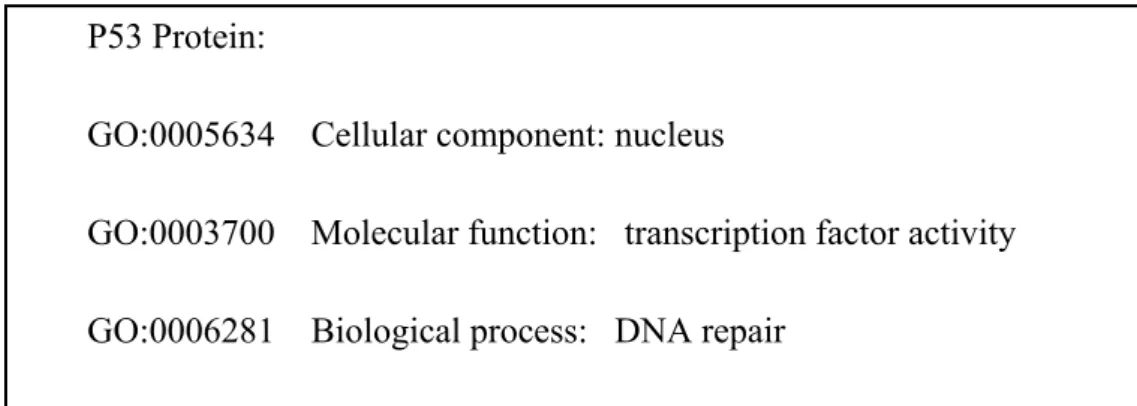
These three categories form a directed acyclic graph (DAG) independently but they have common terms and form a network when represented together. GO terms constitutes a common base for researchers to annotate proteins. Some of GO terms associated with p53 protein can be seen in Figure 6

Figure 6: GO terms associated with tumor suppressor protein p53

P53 Protein:

GO:0005634 Cellular component: nucleus

GO:0003700 Molecular function: transcription factor activity GO:0006281 Biological process: DNA repair

15

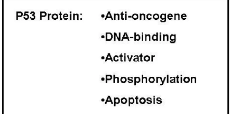
2.3.3 Swiss-Prot Keywords

Swiss-Prot database has a flat set of keywords and uses them to annotate gene products in the database [23]. These keywords are based on structural, functional or other categorical properties of gene sequences. An example annotation can be seen in Figure 7.

16

Chapter 3 Related Work

Currently there is significant data accumulation in molecular biology. This data is in the form of interaction data, gene and gene product annotations, gene expression data, etc. This accumulation gives rise to the need to extract useful information or to derive unavailable information using multiple sources of data.

There is a significant effort in the field to obtain useful information and to analyze these data. Some of these approaches are focused on below topics.

3.1

Protein Function Prediction

Elucidating sequences of genomes of many organisms, functional assignments of these sequences became one of the most important issues in molecular biology. There are several proteins whose functions are not known yet and there are several attempts to attack this problem.

Clare and King modified known machine learning and data mining algorithms such as C45 to learn rules about protein functions of yeast using multiple sources of data [28]. The data sets they used were sequence, phenotype, expression, homology, predicted secondary structure and MIPS functional classification data. They used the derived rules to assign functions to the proteins sequences with unknown function.

In a recent study of Deng et al, an algorithm based on Markov Random Field method is developed to assign protein function using physical and genetic interaction

17 networks of proteins [29]. They used GO terms in function assignment and they assigned GO terms with a probability representing the confidence of prediction, to proteins with unknown function. A similar study to predict protein functions according to GO categories was done by Jensen et al [30]. Sequence data of proteins with unknown functions is used as an input to the algorithm which has been trained with functionally categorized protein sequences before. Function prediction of a protein is not based on sequence similarity but instead the sequence derived features such as post-translational modification sites, protein sorting signals and other physical or chemical properties derived from amino acid sequences.

Clustering has been a widely used method to analyze gene expression data [31] [32]. But elucidation of roles of these clusters remained as a challenge to be taken. Lee et al [33] proposed a graph theoretical modeling of GO terms to interpret gene clusters. First they extracted common GO terms of a cluster of genes and then they found the representative interpretation of the cluster by traversing the GO tree structure they proposed.

3.2

Properties of a PPI Network

Several researchers studied global topology of PPI networks. S. cerevisiae PPI network is shown to have a highly heterogeneous degree distribution and scale free properties. Scale free graphs oppose regular graphs for their small diameter and highly connected neighborhoods compared to graph connectivity. Barabasi and Albert proposed a model for generating such graphs in which a graph is allowed to extend by adding a new vertex, and connecting this vertex to other vertices according to the “preferential attachment” rule, in which probability of connecting the vertex is a linear function of its degree [34]. It has been shown that most biological graphs fall into this category including PPI networks.

The domain reuse could be the reason for preferential attachment, as a protein with “popular domains” would be more likely to get attached to another protein created by gene duplication or obtained a new domain through exon shuffling.

18

3.3

PPI Inference

Even though it is possible to obtain PPI data in a high throughput fashion, it is an expensive and laborious procedure. There are many organisms without any interaction maps or with the maps, which are not complete. The reliability of the experimental techniques is also under discussion. So there are approaches to infer PPIs with computational methods either to support experimental interaction data or to complete interaction maps of organisms.

One approach used to infer PPIs is “interaction mining” which makes use of proteome similarity of closely related organisms. Given experimental interaction map of an organism and whole proteome sequence of the related organism, interaction map of the target organism is inferred using a learning algorithm based on computational statistical learning theory [35]. A previous study to infer the interaction map of an organism was done by Wojcik and Schachter in 2001 [36]. Interaction map of E. coli is predicted from interaction map of H. pylory and its associated protein domains. The inference method used the similarity searches together with clustering based on domain profiles and interaction patterns.

Another method to infer PPIs is protein interaction classification by unlikely protein profiles which is referred to as PICUPP [37]. This method is a statistical approach where the unusual profile pairs are determined if its occurrence in the interaction data is significantly unusual when compared to its occurrence in random protein profile pairing.

PICUPP method is performed independently with different protein profiles as Pfam domains, InterPro [38] signatures and Blocks [39] protein families using the DIP interaction data. After identifying the unusual protein profile pairs putative interacting proteins can be determined.

3.4

Domain Interaction Inference

Another approach using high throughput interaction data is trying to infer domain-domain interactions. Domain-domain interactions can be used to validate

19 PPIs, to obtain functional information to annotate PPIs or to infer interaction networks.

Ng et al developed a computational method to infer domain-domain interactions from interaction data, protein complexes and Rosetta Stone sequences [40][41]. They constructed a database of interacting domains (InterDom) with associated confidence levels for each putative pair of interacting domains.

Li et al used protein interaction data and 3D protein structure of complexes to derive interacting motif pairs [42].

These examples can be extended and there are other studies which do not fall in the above categories. For instance in a study of Segal et al [43] a probabilistic model is developed, which identifies molecular pathways using gene expression and protein interaction data. A pathway is defined to be a set of genes and gene products that function in a coordinated manner to accomplish a specific task.

In another study, Oyama et al tried to extract information on interactions using multiple sources of data available for interacting proteins [44]. Their approach was to discover association rules related to PPIs. Interaction data for the algorithm is created by combining the features of interacting left side protein (LSP) and right side protein (RSP). As a result they obtained rules like:

LSP: Localization = “Nuclear nucleoulus” & Keyword = “nuclease”

⎯→ RSP: Localization = “nuclear nucleoulus” [14, 100.0%]

Rule means proteins having localization “nuclear nucleolus” and keyword “nuclease” interacts with proteins having localization “nuclear nucleolus”. The first number in brackets represents support and the second number represents confidence of this rule. They also discovered rules such as “an SH3 domain binds to a proline rich region”.

20

Chapter 4 Method

4.1

Problem Definition

If we assume that mechanistic basis of each interaction between two proteins is a particular evolutionary innovation (i.e. ab initio formation of a new interaction mechanism), then we can think of the interaction space as a rooted forest, where each root corresponds to an innovated interaction and the other non-root nodes correspond to evolutionary steps this interaction went through. Obviously we observe only a very small subset of this graph, as our PPI data is not complete even for the yeast, let alone a complete evolutionary account. We would like to find and group interactions that belong to the same tree.

In order to infer these groupings, we use a different but closely affiliated evolutionary relation: conserved domains. We assume that each tree has a rule, an ordered pair of set of domains, called relevant domains that must be satisfied by all interactions in the tree. In order to satisfy a rule, corresponding proteins of the interacting pair must have a superset of corresponding relevant domain set.

The problem is complicated by the fact that in eukaryotes, a protein takes part in an average of 5-8 interactions. Therefore not every domain of a protein is relevant to the interaction. For example, ERBB2 has 13 pfam domains (Figure 8), and is also known to be interacting with several proteins [45] including cyclin Bs. It interacts

21 with cyclin B’s C-terminal domain via its protein kinase domain. Its other domains are involved in different interactions.

Figure 8: Domains of ERBB2 according to Pfam.

We assume that each interaction between two proteins exists for a particular mechanism, which can be represented as a specific domain signiture, so each interaction should be a member of a single cluster. Even though an interaction might occasionally satisfy rules of two or more clusters, the underlying cause of that interaction should be based on a certain conserved mechanism, preferably defined by a single cluster rule. We call the features of the protein that are relevant to this conserved mechanism active features for this interaction. (e.g. in ERBB2-cyclin B interaction protein kinase domain of ERBB2 is active whereas other domains are inactive.)

Given

− a set of features (domain features for this study) D = {d1,..., dm},

− a set of proteins P = {p1,..., pt}, where every protein is defined by a set of

features, D(pi) ⊆ D,

− a set of PPIs I = {i1,..., in}, where ij is an ordered pair of proteins, ij ∈ P x P ,

We would like to partition interaction set I to clusters such that interactions in the same cluster share the same conserved mechanism. We also aim to extract the rules which are composed of active features, describing interaction clusters. Formally we can model this problem as

to find a clustering C = {c1,…,ck}, where ci ⊆ I,

Υ

k i i I c 1 = = and ci ∩ cj = ∅ for

22 H=

∑ ∑

∑

and αd ,iis 1 if domain d is active in interaction i, 0 otherwise.

Obviously we do not know the α function and we will need some heuristics to estimate it.

4.2

Clustering Approach

Our approach to attack the above problem is to cluster PPIs with Expectation Maximization (EM) algorithm [46] and to assign descriptive rules to interaction clusters by observing cluster parameters.

In data mining it is not usually possible to describe the data by a single probabilistic or parametric model. Real life data is usually in the form of a mixture of different distributions and it is modeled as linear combination of multiple distribution functions. EM is one of the approaches used to solve such mixed models. Another property of such data is that it may not be possible to observe or determine all features of data instances. There may be missing features in some instances of data or a feature might not be observed at all. EM also performs well with unobserved features.

EM is a general iterative optimization algorithm, which maximizes a likelihood score function, given a probabilistic model with possibly missing data. Likelihood score function is a measure of how well the model fits and explains the data. In our problem, cluster labels are missing data and the probabilistic model is the mixture of different distribution functions of clusters. EM algorithm iterates between expectation (E) and maximization (M) steps until it satisfies some predetermined condition. In the expectation step, missing data is predicted using the computed parameters of the mixed model. In our problem we calculate membership probabilities of interactions in the E step. Parameters of the mixed model are computed in the M step using the calculated missing data of E step as well as observed features of the instances. These parameters are calculated to maximize the likelihood function. At the beginning of the algorithm either parameters of the model

23 or the missing data are assigned. This assignment might be random or some more intelligent assignment might be performed. Then algorithm starts from the step which would use these assignments. In our approach we prefer to assign missing data (membership probabilities) randomly and start from the maximization step which computes parameters using this random assignment.

4.2.1 Probabilistic Model

We have a set of interactions I = {i1,..., in}. We assume that each interaction

belongs to precisely one of k clusters. We represent this as an attribute of i such that i.C ∈{1,…, k}, where i.C variables are hidden variables of our model which we aim to determine in this study.

As given in the problem definition, each protein p is represented by its features. Each protein has a discrete-valued (0/1) m=|D| variables, ‘1’ representing a present feature, ‘0’ representing an absent one. Since interactions are ordered pairs of proteins, interaction i is represented by 2m variables, first m variable defining the features of the first interacting protein (protein-A), second m defining the features of the second one (protein-B). We use Naïve Bayes Model and we assume that these attributes are conditionally independent.

Equation 1 represents the model of observing interaction i as a member of cluster p given the parameters ωp of cluster p, where i.Vj represents the value of jth

attribute of interaction I and ωp,j represents the parameter of cluster p for attribute j.

⎟⎟ ⎠ ⎞ ⎜⎜ ⎝ ⎛ =

∏

∏

Since the attributes are assumed to be conditionally independent, this model can be represented with the multiplication of individual probabilities of observing 1 for the jth attribute in the pth cluster. Denoting this probabilityωp, density function for the pth _{cluster can be written as:}

k p V i P j iVj j p V i j p j p j p = − < < − 1 , ) 1 ( ) | . ( ω _, ω ._, ω _, 1 . (2)

24 The equation for observing interaction i in our data set can be expressed as the weighted sum of these cluster densities

∑

∏

∏

∑

where πprepresents the probability of cluster p (0≤πp ≤1 and

∑

p πp

A.0.1.5 Expectation Step

In the expectation step of the EM algorithm we try to assign interactions to clusters. We do this assignment by computing the probabilities that an interaction i belongs to each cluster. Let P(i.C = p) be the probability that interaction i belongs to cluster p. By Bayes rule and given fixed set of parameters ω and π, this probability can be written as:

) ( ) 1 ( , ) 1 ( min . ) . ( 2 1 . 1 , . , 1 . 1 , . , i P p C i P m m j V i j p V i j p m j V i j p V i j p p j j j j ⎟⎟ ⎠ ⎞ ⎜⎜ ⎝ ⎛ − − = =

∏

∏

A.0.1.6 Maximization Step

In the Maximization step of EM algorithm we compute the new parameters which fit better to the cluster assignments done in the previous expectation step. New parameter matrix ωnewfor interaction attributes are computed as follows:

∑

∑

New cluster probability parameter vector πnewis computed as follows:

∑ ∑

∑

25 We will iterate on E and M steps until the difference between new and old parameters is smaller than some predetermined threshold.

4.2.2 EM Algorithm

Basic idea of the algorithm and some definitions that will be used throughout this section are as follows.

We run EM algorithm multiple times to be able select the best clustering among multiple runs. At each EM run we iteratively perform E and M steps. In the E step we try to assign cluster membership probabilities of interactions which are represented by hidden_clusters. hidden_clusters is a 2D array of size nof_interactions x nof_clusters. In the M step we try to compute parameters of our mixed model, which are weights and phi. weights is a 2D array of size nof_clusters x nof_features, phi is an array of size nof_clusters. These two arrays correspond to ω and π of the probabilistic model, respectively. Maximization step also computes the mean_weight_difference value, which is the mean of the differences of the new values and the previous values of weights array.

EM iterates until this mean_weight_difference is smaller than a predetermined threshold which is 10-9 for our study.

Two arrays are introduced to decrease complexity of the algorithm. One is

feature_interaction_mapping of size nof_features and each element

feature_interaction_mapping(j) holds a list of interactions containing feature j. The other is present_features of size nof_interactions. present_features(k) holds the present features of interaction k.

algorithm RUN_EM

1) for i =1 to i= nof_runs

2) call DO_EM()

3) write output 4) write entropies

26

algorithm DO_EM

1) call INIT_CLUSTERS

2) mean_weight_difference : = call DO_MAXIMIZATION

3) while mean_weight_difference greater than mean_weight_difference _threshold 4) and nof_iteration smaller than max_nof_iteration

5) call DO_EXPECTATION

6) mean_weight_difference : = call DO_MAXIMIZATION

7) increase iteration by 1

algorithm INIT_CLUSTERS

1) for i = 1 to nof_interactions

2) for j = 1 to nof_clusters

3) hidden_clusters(i,j) randomly determine probability

4) normalize probabilities for each interaction

algorithm DO_MAXIMIZATION

1) for p = 1 to p= nof_clusters

2) for j = 1 to j= nof_features

3) compute weights(p,j) using

∑

∑

4) compute phi(p) using

∑

∑

∑

∏

∏

27 where i∈ present_features(k) and 1 ≤ i ≤ nof_features/2,

j ∉ present_features(k) and 1 ≤ j ≤ nof_features/2. 3) proteinB =

∏

∏

where i∈ present_features(k) and (nof_features / 2 +1) ≤ i ≤ nof_features,

j ∉ present_features(k) and (nof_features / 2 +1) ≤ i ≤ nof_features.

4) hidden_clusters(k,p) = phi(p) . min (proteinA, proteinB)

5) normalize hidden_clusters(k)

4.3

Complexity Analysis

Let's denote the number of clusters with k, interaction data size with n and number of domain features with m.

Complexity of the expectation step:

In the expectation step, for each interaction we calculate Equation 4. A naïve approach takes Θ(kmn) steps as we have to iterate over all clusters and domains for each interaction. However we observe that domain features are very sparse. In order to take advantage of this fact we calculate, membership probability of a domainless protein for each cluster:

∏

∏

We calculate this once per iteration and it takes Θ(km) time.

28

∑

∏

∏

∏

∏

Let’s denote the number of domain instances in all interactions with Μ i.e. the number of 1s in our sparse interaction-domain matrix. If we use appropriate data structures (such as a vector of linked lists instead of an array), then complexity of evaluating Equation 4 becomes Θ(km + kM). If we denote average number of domains per interaction with µ=M/n, where µ<<m, expectation step complexity takes the final form of Θ(km + nkµ).

Complexity of the maximization step:

In the maximization step, for each cluster we calculate Equation 5. Naively calculating Equation 5 takes Θ(knm) steps as we have to iterate over all interactions and domains for each cluster. Again we take advantage of sparseness property and for each domain we consider only interactions where this specific domain is found. We calculate, total of membership probabilities of all interactions for each cluster:

∑

in Θ(kn) steps. Then for each domain we calculate membership probabilities of interactions having this domain.

p V i t new j p j t p C i P σ ω

∑

If we use appropriate data structures (such as a vector of linked lists instead of an array), then our complexity becomes Θ(kn + kM). Our maximization step complexity takes the final form of Θ(kn + knµ)= Θ(knµ).

29

Overall complexity:

We iterate over alternating E and M steps for e epochs. Thus the complexity becomes:

Θ(e(km+knµ))

where µ is scale free and can be considered as a constant for each organism; thus we finally have Θ(ek(m+n)).

There is no hard limit on the number of epochs needed for convergence. However since EM is a hill-climbing algorithm, it is guaranteed to converge. For hypothetic and real sample clustering, so far we never needed more than 100 epochs. For the entire real data set available, clustering into 40 clusters can be achieved in the order of 100 epochs. However for large number of clusters such as 400, 5000 epochs was not sufficient for the convergence of the algorithm. Optimizing cluster number and mean weight difference threshold might solve the convergence problem.

30

Chapter 5 Results

To test the performance of the algorithm we initially performed our studies on hypothetic data where we do the cluster assignments of interactions ourselves. So we could compare the results of our clustering algorithm with the actual assignments.

5.1

Hypothetic Data

We prepare the hypothetic data for given number of interactions (n), number of features of an interaction (2m) and number of proteins (t).

First we determine the cluster rules, which are common active features of interacting proteins within a cluster. We do this by assigning features to be active features with certain probability. This probability value is decided according to the properties of the real data. We expect to see about 2-6 active features per interaction. This expectation is based on the fact that yeast has ~5 domains per protein. Proteins have multiple functions and different domains or combinations of domains serve different functions and mediate different interactions. So a protein can allocate 1-3 domains to a single interaction on average. This results in 2-6 active features in an interaction on average.

In this study we determined the number of active features as 4 on average, ensuring the presence of at least 2 active features, one on protein-A, the other on protein-B side of an interaction rule. So first we determined one active feature for

31 each protein description of a rule and then assigned activity to the other features with probability

(4(average) -2(ensured)) / 2m (feature size) = 1/m.

Rule assignment corresponds to determination of ω matrix of the EM algorithm. After cluster rule assignment, cluster probability assignment is done by assigning random values to each cluster and normalizing afterwards. This property corresponds to π vector.

Interactions are created after determining parameters of clusters. For each interaction its cluster assignment is determined according to cluster probability vector and two proteins (protein A and B) are randomly selected to participate in that interaction. At the beginning, all values of m features defining a protein are 0. When a protein is selected to be protein-A of an interaction, its features are updated according to the assigned cluster rule and active features among first m features of the rule vector are updated to be present in protein-A. Active features among remaining half of the rule vector are updated to be present in protein-B.

This process is performed until all interactions are assigned to some cluster and their interacting protein pairs are determined. For every interaction protein features are updated according to cluster rules.

This model treats interactions as ordered pairs, for example we expect all kinases on the left position and all their targets on the right. Obviously this is not the case with the real data. As a workaround, we introduce two ordered pairs (a,b) and (b,a) in order to represent unordered pair {a,b}. As a side effect we expect symmetric clusters with a perfect clustering. At the end we obtain a hypothetic data set of 2n interactions of 2k symmetric clusters.

5.2

Real Data

We obtained our interaction data set using BIND data. BIND has multiple types of interactions such as protein-DNA and protein-RNA as well as PPI. In addition it is not a single organism database. We extracted 5817 PPIs of Saccharomyces cerevisiae

32 from BIND data. These 5817 interactions are among 3620 proteins. We prepared a relational database of interactions and populated this database with the information available for proteins in public databases. We annotated the proteins with Pfam domains, GO terms and Swiss-Prot keywords. For this study we use only Pfam domain compositions of proteins as the feature set describing a protein.

Interaction data is written on a text file, which would be input to the clustering algorithm. Each interaction constitutes a single line of two times the feature set size of characters in data file, first feature set signifying protein-A, second signifying protein-B. Each character is either ‘1’ or ‘0’ corresponding to presence or absence of features respectively.

5.3

Clustering Evaluation

We have three measures to evaluate clustering and the clusters. They are all based on statistical entropy measures [47].

5.3.1 Statistical Entropy

Our clustering algorithm computes a 2D array of probabilities called hiddenClusters. Rows correspond to interactions and columns correspond to clusters. So the element at position (i,j), hiddenClusters(i,j), defines the probability of interaction i to belong to cluster j. For an interaction the sum of probabilities is 1.

In our statistical entropy measure we assign interactions to its most probable cluster. Then for a cluster we measure the entropy of cluster cp as

∑

where k is the number of hypothetic clusters and xi is the ratio of number of

interactions which belong to hypothetic cluster hi to the number of elements of

cluster cp: | | | | p p i i c c h x = ∩

33

5.3.2 Probabilistic Entropy

With this measure, different from the measure above we do not assign interactions to the clusters with the highest probability; instead we use probabilistic values:

∑

where cp is the cluster, of which we measure the entropy, k is the number of

hypothetic clusters and xi is calculated using

(

)

(

)

∑

∑

5.3.3 Unsupervised Entropy

The above measures can only be used in the presence of information of hypothetic or real cluster information. But we need to have a measure to evaluate the clusters when we do not know the real clusters which would be the case for our real data. So we developed an entropy measure for an unsupervised clustering.

We computed entropies of each cluster cp, as the total of multiplication of each

interaction probability to be in that specific cluster with the entropy of that interaction: UnsupervisedEntropy =

∑

(

)

where entropy of an interaction is computed from probability distribution of that interaction using

∑

34

5.4

Hypothetic Data Results

We prepared hypothetic data of different numbers of interactions, features, proteins and clusters. Then we clustered the hypothetic interactions with EM algorithm for multiple runs and compared the total entropies to choose the best clustering with the lowest entropy.

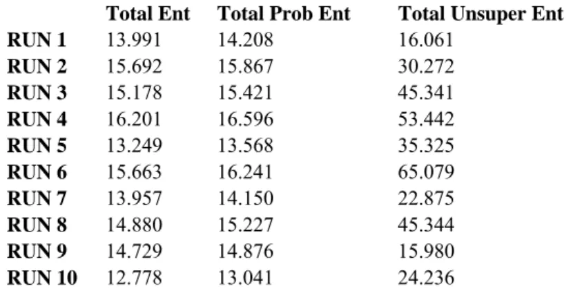
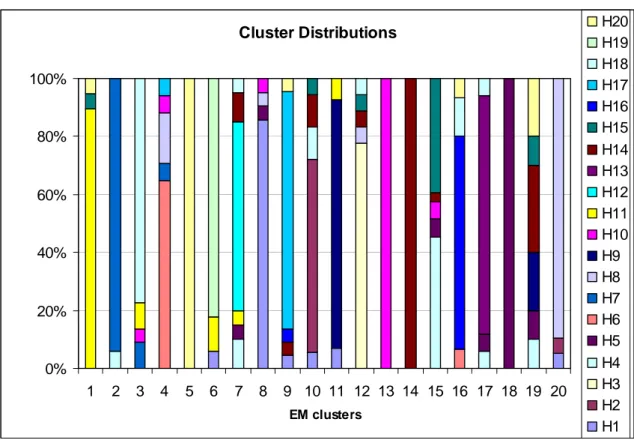
Our first clustering results are with 400 interactions belonging to 20 clusters. Interactions were among 1000 proteins with 500 features representing them. EM clustering algorithm is run 10 times and the total entropy measures of clusters for each run are shown in Table 1. According to total statistical entropy and total probabilistic entropy measures last run scores lowest, which suggests that run 10 gives the best clustering among the 10 runs. Figure 9 shows the distributions of the members of the clusters obtained as the result of last EM run. Members of a cluster are determined by assigning an interaction to its highest probable cluster. Each bar represents what percent of the members of that cluster originates from which hypothetic cluster. Colors represent hypothetic clusters.

Total Ent Total Prob Ent Total Unsuper Ent

RUN 1 13.991 14.208 16.061 RUN 2 15.692 15.867 30.272 RUN 3 15.178 15.421 45.341 RUN 4 16.201 16.596 53.442 RUN 5 13.249 13.568 35.325 RUN 6 15.663 16.241 65.079 RUN 7 13.957 14.150 22.875 RUN 8 14.880 15.227 45.344 RUN 9 14.729 14.876 15.980 RUN 10 12.778 13.041 24.236

Table 1: Total entropy values calculated for each run of the algorithm. Total statistical entropy and total probabilistic entropy show similar pattern, whereas the unsupervised entropy behaves differently. According to first two

35 Cluster Distributions 0% 20% 40% 60% 80% 100% 1 2 3 4 5 6 7 8 9 10 11 12 13 14 15 16 17 18 19 20 EM clusters H20 H19 H18 H17 H16 H15 H14 H13 H12 H11 H10 H9 H8 H7 H6 H5 H4 H3 H2 H1

Figure 9: Cluster distribution of hypothetic data of 400 symmetric interactions (A-B and B-A) of 1000 proteins. Each protein is defined by 500 features. Interactions are created according to 20 cluster rules without introducing any error to the rules. This figure represents cluster distributions of clusters obtained by EM. Each bar represents percentage of members coming from hypothetic clusters and colors represent hypothetic clusters. Color hypothetic cluster mapping is given with the legend on the right.

36

Stat Ent Prob Ent Unsuper Ent EM 1 0.409459 0.413097 0.49244826 EM 2 0.223718 0.240408 0.0302038 EM 3 0.775714 0.780758 0.17848597 EM 4 1.087761 1.092503 0.15379087 EM 5 0 1.27E-05 3.03897891 EM 6 0.578325 0.554874 0.64984492 EM 7 1.189886 1.210222 0.19090528 EM 8 0.567061 0.665109 1.26900196 EM 9 0.726193 0.726246 0.02112411 EM 10 1.079735 1.079735 1.46E-14 EM 11 0.509137 0.523422 1.08281205 EM 12 0.837772 0.837772 8.05E-25 EM 13 0 4.12E-09 2.39814848 EM 14 0 1.43E-13 3.03764265 EM 15 1.171123 1.26529 5.59577996 EM 16 0.857174 0.862877 0.00266242 EM 17 0.659872 0.659505 0.03115513 EM 18 0 1.84E-11 3.61538726 EM 19 1.695743 1.721635 2.01557814 EM 20 0.409459 0.407506 0.43181102

Table 2: Entropy measures. Three different entropy measures of each

clusters obtained at the 10th run of the clustering algorithm. Statistical entropy

values and probabilistic entropies give similar results. Cluster 5, 13, 14, 18 have the lowest entropy values according to first two measures.

As seen in Table 1 and Table 2, unsupervised entropy measure shows an unpredicted behavior. This may be the result of a wrong assumption about the properties of clusters. We will not be using that measure to evaluate clustering in this study.

When we observe Figure 9 and Table 2, clusters 5, 13, 14 and 18 have homogenous composition and thus the lowest entropy measures. In these clusters we expect to observe similar or same rules to corresponding hypothetic clusters. Matching cluster rules can be seen at Table 4. 18 of the hypothetic cluster rules are identified with quite high weights. Even the cluster compositions are not homogenous in the sense of hypothetic clusters, the rules are determined with very high rate.