Adaptive control of flexible multilink manipulators

Adaptive control of flexible muItilink manipulators

MEHMET BODURt and M. EROL SEZER*

An adaptive self-tuning control scheme is developed for end-point posinon control of flexible manipulators. The proposed scheme has three characterist-ics. First, it is based on a dynamic model of a flexible manipulator described in cartesian coordinates, which eliminates the burden and inaccuracy of translat-ing a desired end-point trajectory to joint coordinates ustranslat-ing inverse kinematic relations. Second, the effect of flexibility is included in the dynamic model by approximating flexible links with a number of rigid sublinks connected at fictitious joints. The relatively high stiffness of the fictitious joints is shown to result in a decomposition of the model into two subsystems operating at different rates. This allows for stabilization of the oscillatory modes associated with the flexible links by a fast feedback control in addition to a slower control for trajectory tracking. Third, the control is constructed from measurements of the end-point position and deformations of the flexible links, with the manipu-lator parameters required to form the control obtained using a recursive least-squares estimation algorithm, which is fast enough for on-line applica-tions. Satisfactory results are obtained from digital simulation of a two-link flexible manipulator.

1. Introduction

Conventional industrial manipulators are usually made stiff and bulky to avoid vibrations and thus to achieve precision in motion control. Several considerations such as lower arm cost, higher motion speeds, better energy efficiency, safer operation, and improved mobility resulted in a new generation of manipulators with lightweight, flexible links (Book 1985). Two major prob-lems in the motion control of flexible manipulators are to avoid oscillations due to flexibility distributed along the links and to achieve accuracy in the position-ing of the end-effector.

While several control schemes have been established for rigid manipulators (see, for example, Luh et al. 1980, Freund 1982, Balestrino et al. 1983, Koivo and Guo 1983,Lee and Lee 1984,Slotine 1985,Koivo 1985, Souissi and Koivo 1987,Craig 1988), a direct application of these schemes to flexible manipulators gives unsatisfactory results owing to neglected elastic modes. Effective control of flexible manipulators requires inclusion of elastic modes in the dynamic model (Book 1984, Judd and Falkenburg 1985, Cetinkut et al . 1986), and additional control to stabilize these vibrational modes. The singular perturbations approach (Kokotovic 1984) based on a decomposition of the manipulator dynamics into slow and fast modes associated with the joint variables and elastic deformations has been reported to give satisfactory performance (Siciliano and Book1988).

Another difficulty associated with the control of flexible manipulators is the Received 26 March 1992. Revised 16 August 1992.

tDepartment of Electrical and Electronics Engineering, Middle East Technical University, Ankara, Turkey.

*

Department of Electrical and Electronics Engineering. Bilkent University. Ankara, Turkey.

0020-7179/93 $10.00©1993 Taylor&Francis Ltd

solution of inverse kinematic relations in order to express a desired end-point trajectory in terms of joint variables. Although it is possible to calculate the static deflections of the links due to gravity at every point of a specific trajectory, this is a tedious task as all calculations have to be redone for each new trajectory. Besides, deflections of the links during fast motions do not exactly match the precalculated static deflections. The pseudo-link concept introduced by Nemir et al. (1988) allows for a simple description of the end-point trajectory in terms of pseudo-link angles, considerably simplifying the inverse kinematics problem. The pseudo-link angles needed for feedback purp-oses are obtained from the measurements of the joint angles and of the deflections of the links using strain gauges attached to them. The pseudo-link concept has also been used by King et at. (1990) in a two-time-scale approach to control of flexible manipulators, which promotes the application of model reference adaptive control schemes (Craig 1988).

An obvious way of avoiding the inverse kinematics problem is to model the manipulator dynamics and describe the desired trajectory in cartesian base-frame coordinates. Although end-point position control in cartesian and other task-ori-ented coordinates has been studied by many researchers (e.g. Luh et at. 1980, Takegaki and Arimoto 1981, Koivo 1985), the resulting control schemes require extensive computational effort, and are, therefore, impractical for real-time applications.

The objective of this paper is to develop a computationally attractive adaptive scheme for end-point position control of flexible manipulators suitable for on-line applications. For this purpose, flexible links are modelled by a simple bulk approximation using a series of fictitious joints, which represent lightly damped vibration modes. This bulk approximation allows for the derivation of dynamic equations of a flexible manipulator using the systematic formulations such as Lagrangian (Uicker et at. 1964), or generalized d'Alernbert (Lee et al. 1983), developed for rigid manipulators. Using the jacobian of the bulk approximated rigid manipulator, the dynamic equations are expressed in terms of cartesian end-point variables and fictitious-joint angles. The resulting model is discretized into an auto-regressive externally excited system, which is shown to possess a two-time-scale property. This allows for a decomposition of the control law into two parts, one to force the slow system describing the end-point dynamics to track a desired trajectory, and the other to stabilize the fast subsystem describing the vibrational dynamics. The slow control consists of a feedforward computed-torque component and a feedback from cartesian track-ing errors, as standard in motion control of rigid manipulators (Koivo 1989). The fast control, which is a feedback from the fast components of the fictitious-joint variables, is approximated by a feedback from the actual (measured) fictitious-joint variables and their quasi-constant components, which can be expressed in terms of the end-point variables.

Implementation of the derived control law requires that the manipulator parameters be known at every point of the trajectory. They can either be calculated from the measured end-point variables and link deformations using the employed formulation, or be estimated using an on-line adaptive scheme. The latter involves much less computational effort, and is, therefore, more suitable for on-line applications.

The developed control scheme is tested by digital simulation of a two-link

manipulator with a flexible first link. The simulations are carried out in two groups. The first group consists of simulations of collocated control schemes without and with compensation of the static torque due to gravity. The second group includes simulations of the developed control scheme with the manipula-tor parameters computed from the bulk model using the generalized d' Alembert formulation, and with the parameters obtained by a recursive least-squares estimation (RLSE) algorithm (Goodwin and Sin 1984) to obtain a self-tuning regulatory control. Simulation results indicate that the self-tuning approach can be successfully implemented in real-time position control of flexible manipula-tors.

2. Dynamic modelling

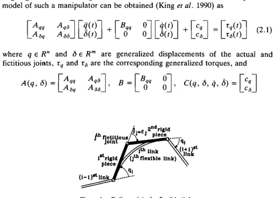
The dynamics of a flexible link can be accurately modelled as a distributed parameter system resulting in a set of partial differential equations and initial/ boundary conditions as given by Cannon and Schmitz (1984). Such a model describes an infinite number of modes, and is extremely complicated for practical use. Studies by Cannon and Schmitz on identification of finite-order transfer functions of flexible links showed that the modal gains beyond the third flexible mode are negligible. Thus, the dynamics of a flexible link can ade-quately be approximated by a second-order bulk model, which consists of two rigid sublinks joined by a fictitious joint as shown in Fig. 1. Note that the angular displacement of the fictitious joint is a measure of the deflection of the link.

Consider a flexible manipulator consisting of n joints, and let the m flexible links (m,,;; n) be modelled by second-order bulk approximations. Using the Lagrange-Euler or the generalized d'Alembert formulations, the dynamical model of such a manipulator can be obtained (King et al. 1990) as

where q E R" and 0 E R'" are generalized displacements of the actual and

fictitious joints, 'q and 'Ii are the corresponding generalized torques, and

A(q, 0)

=

[~~: ~~:l

B

=

[B<iq

~l

ct«.

0,

q,

c5) =

[~~J

Figure 1. Bulk model of a flexible link.

are, respectively, the non-singular matrix of inertial coefficients, the matrix of the damping coefficients of the actuators at the actual joints, and the vector of coriolis, centrifugal and gravitational torques. The actuator torques, 'rq(t), in (2.1) are external inputs to the manipulator and can be chosen freely within the limitations of the actuators. The torques of the fictitious joints, however, are determined by the internal dynamics of the flexible links as

(2.2) where Ks=diag{Ks1' ... , Ksm } and Kd=diag{K d1, ... , Kdm} contain the

spring constants and the viscous dampings of the fictitious joints.

Equations (2.1) and (2.2) constitute a dynamic model of a flexible manipula-tor in the joint coordinates. To obtain a model in cartesian coordinates, we assume that the end-point displacement vector pet) has the same dimension as q(t), and write Accordingly

[~]

=

[~q ~o] [~]

[~]

=

[~q ~o]

D]

+

[~q

(2.3) (2.4)

where !q=3t/3q, jq= 12:7=1(32jJ3qj3qMI

+

2:~1(32jJ3qj3bl)t5dn.n, and

J0 and J0 are defined similarly. To avoid pathological cases, we assume that the

jacobian Jq(q, b) is non-singular and well-conditioned along the desired trajec-tory so that the mapping in (2.3) is invertible. Applying the transformation in (2.3) to the model in (2.1) and (2.2), we get

where

Ape]

[~(t)]

+

[Bpp

A ee c(t) 0 B

t ]

[~g?J

+

[~:]

=

[-Ksc(:)q~)

Kd£(t)] (2.5)

(2.6)

where the terms involving jq and

t,

are included in cp and Ceo Note that the identity e = _{b is used only to change the notation so that A ee in (2.5) is} distinguished from A

_oo

in (2.1). Note also that while B

_qo

= 0, B_pe

'*

O.

Finally, we discretize (2.5) to get

T-2Appli2Pk

+

T-2A peli2Ck

+

T-1BppliPk

+

T-1Bpelick

+

Cp= 'rk } (2.7)

T- 2A epli2pk

+

T-2Aeeli2ck

+

KsCk

+

T-1Kdlick

+

C_e=0

where Pk= p(kT), Ek= E(kT), and T:k = T:q(kT) with T being the discretization step, the difference operator ~ is defined as

(2.8) and the subscript k is omitted from the time-varying coefficients A pp, ... , Bpp c_p and C_efor simplicity in notation.

3. Anon-collocated two-time-scale control

It has already been shown by Siciliano and Book (1988) that, for sufficiently large values of the spring constants of the fictitious joints, the joint-space model in (2.1) possesses a two-time-scale property. Although the analysis of Siciliano and Book (1988) can be imitated for the cartesian-space model in (2.5) to obtain a composite control consisting of slow and fast parts, which is then suitably discretized for use in (2.7), we prefer to derive the control law directly using the discrete-time model in (2.7) for the purpose of discrete implementation of the adaptive controller.

We assume that elements of K, are sufficiently large compared with other parameters in (2.7), and write K, = T-2K;. As shown in the Appendix, the system has a two-time-scale property, which allows for a decomposition of the variables into quasi-constant and fast components as

Pk '" ih, Ek '" Ek

+

£b T:k'" T:k

+

Tk

Accordingly, (2.7) is decomposed into two subsystems: T- 2App~2ih

+

T-1Bpp~ih

+

cp

=

T:k describing the slow dynamics, and

~2£k

+

EeeK;£k

=

T2EepTk

describing the fast dynamics, where

(3.1)

(3.2)

(3.3)

(3.4)

The quasi-constant component of Ek is specified in terms of ih and T:k as

Ek

= -

K;I[AepA ;;(T:k -

r :'

Bpp~ih - cp)

+

cel

(3.5)

At this point it is appropriate to note that, as in all applications of singular perturbations theory, whether a parameter could be considered to be 'large' relative to others depends on the eigenstructure of the system rather than its absolute magnitude. Although our theoretical development above formally shows that the assumption K;

=

T-2_{K; leads to a separation of the time scales}

of the system, the validity of this result should be verified either by a simulation or by actual implementation.

The above decomposition of the manipulator dynamics into slow and fast components is valid only if the fast subsystem in (3.3) is asymptotically stable. To achieve stability of £b we apply a fast feedback control of the form

(3.6)

which results in

(I + EEEK;)'ek - (21 + _{T 2E EPI<I)'ek_l} + (I - _{T 2E EpI(2)Ek_Z} = 0 (3.7)

From (3.7) we observe that if I<1and I< Z are chosen to satisfy

A

2

A }

EEpK 1

=

-T- [(I

+

EEEK;)ZI

+

2I]

A 2 A (3.8)

EEpK2 = -T- [(I

+

EEEK;)Z2 - I]

then the closed-loop fast subsystem is described by

Ek

+

Z,Ek-l

+

ZZEk-2

=

0 (3.9)

Now

Z

1 and

Z

2 can be chosen arbitrarily to stabilize the fast subsystem by placing its 2m poles at desired locations. Note that this also allows for decoupling of the fast dynamics, which means the vibrational modes associated with the fictitious joints can be controlled independently. We also note that since the bulk approximations of the flexible links contain only a single fictitious joint, we have m~ n ,so that equations in (3.8) are generically solvable for I<I

and

1<2'

With the fast subsystem stabilized, it now remains to choose the slow component of the control input 'k to achieve a satisfactory performance of the slow subsystem in (3.2). This, however, is the standard tracking problem for rigid manipulators, for which a solution is available (Koivo 1989): We simply choose

1:k

=

T- 2A pptl2pi

+

T- 1Bpptlpi

+

Cp

+

K

,e~-l

+

K

2e~-2 (3.10)

where

pi

describes the desired trajectory of the end-point, and e~=

pi -

J5

k is

the deviation of the actual trajectory from the desired one. Note that the first three terms in (3.10) constitute a feedforward control (computed torque) which decouples the manipulator's slow dynamics, and the last two terms form a feedback control to achieve a desired performance of the decoupled dynamics. Applying the control in (3.10) to the slow subsystem in (3.2), and rearranging the terms, we obtain

p 2 - P 2 - p

(A pp

+

TBpp)ek

+

(-2A pp - TB pp

+

T K l)ek-l

+

_{(A pp}

+

_{T K 2)ek-2}

=

0

(3.11) Letting (3.11) is reduced to

~l

=

T~~[App

+

(~:p

+

TB pp)(2 1

=

l)] } K 2= T Bpp

+

T (A pp

+

TB pp)(Z2 - l) (3.12) e~

+

21e~-1

+

22e~-2 = 0 (3.13)

Clearly, the error dynamics described by (3.13) can be controlled as desired by choosing

2

I and

2

₂properly to place the 2n poles arbitrarily.

The composite control is the sum of the fast and slow controls in (3.6) and (3.10). Since Ek is not directly measurable, we approximate Tk in (3.6), by using

Ek "" Ck - £kand letting£k-l ""£k-Z~ £b as

(3.14)

Now the expression for Ek in (3.5) can be used in (3.14) to get

rk

=

K1Ek-l

+

KZEk-Z

+

(K 1

+

Kz)K;I[AEpA;;(Tk - T- 1Bpp/).jh - cp)

+

c E]

which, like the slow control Tk> involves only measurable variables.

(3.15)

4. Adaptive self-tuning non-collocated control

Implementation of the control law derived in the previous section requires that the manipulator parameters A pp, ... , Bpe> cp and CE be known. If the desired trajectory is known beforehand, then these parameters can be calculated and stored off-line at several points along the trajectory: under the assumption of perfect tracking without any oscillations, we set Pk= ih= pi and Ek= 0, so that e~

=

0 and

10k = Ek = -K;I(T-zAEP/).ZPk

+

cE )

which is obtained by substituting (3.10) with e~

=

0 into (3.5). Using inverse kinematic relations, actual and fictitious joint displacements qk and Dk are

calculated from P« and 10k> which, in turn, are used to calculate the parameters Aqq , . . . , Bqq in (2.1), and finally App, ... , BPE in (2.7) via (2.6). Obviously, this method involves extensive computations which are not suitable for on-line applications.

An alternative to calculating the manipulator parameters is to estimate them from input/output data using the RLSE algorithm (Goodwin and Sin 1984). To reduce the computational effort, we make a simplifying assumption that B_pp

=

0 and B_PE

=

O. Then, defining

Uk

=

T-1/).pk> Wk

=

T-1/).Ek (4.1)

which represent the approximate cartesian velocity of the end-point, and the angular velocities of the fictitious joints, respectively, (2.7) becomes

(4.2)

Letting

Equations (4.2) can be written in the standard form Yk

=

fh</>k

where Ykis the observation vector

</>k

=

luI

I]T is the input, and

fh

=

[E k - TEkcd

is the parameter matrix, with E; denoting the matrix in (3.4).

(4.3)

(4.4)

Assuming slow variations of the parameters, a least-squares estimate of

e

_k which minimizes the weighted sum

k

h

=

2:

yk-I(y/ - e/¢/)T(y/ - e/¢/) (4.5)

/=0

is obtained (Goodwin and Sin 1984) as

~ ~ ~ T }

e k

=

e k- I

+

£Yk(Yk - e k_1¢k)¢kPk-1

(4.6)

Pk

=

y-I(Pk-1 - £YkPk-l¢krpIpk- l)

where £Yk

=

(1

+

rpIPk-l¢k)-I, and 0< y,,;;1 is the forget factor.

In (4.6), the input vector ¢k is constructed from the calculated value of the input torques, T:b and the measurement of the deflections, Eb of the fictitious joints. Once

e

_k is calculated, estimates of the parameters A_{pp , ••• ,} Am c_p and c, are obtained by inverting the (n

+

m) x (n

+

m) matrix Ei,

In implementing the RLSE algorithm, the initial value of

e

k can either be

calculated using inverse kinematic relations at the start of the trajectory assuming static deflections, or obtained by a (n

+

m

+

Ij-step non-recursive least-squares estimation scheme. It may also be necessary to add suitable continuous persistent oscillations to the input T:k in order to excite all the modes

of the manipulator (Goodwin and Sin 1984).

With the manipulator parameters estimated, the slow control is given by tk = T-2A~p[~2p~

+

(21

+

2I)e~_1

+

(22 - IM-2]

+

c~ .(4.7) which is obtained from (3.10) and (3.12) with _Bpp

=

0, and superscript e denoting the estimated value of the indicated parameter. Substituting (4.7) into (3.15), the fast control becomes

A A A . . . -1 e

1:k =KIEk_1

+

K2Ek-Z

+

(K I

+

Kz)Ks c,

Z~ ~ I e Z d - P - P

+

T- (K I

+

Kz)K; A,p[~ Pk

+

(21

+

2I)ek_1

+

(2z - I)ek-Z] (4.8)

The expressions for tk and 1:k above show a further advantage of assuming

Bpp

=

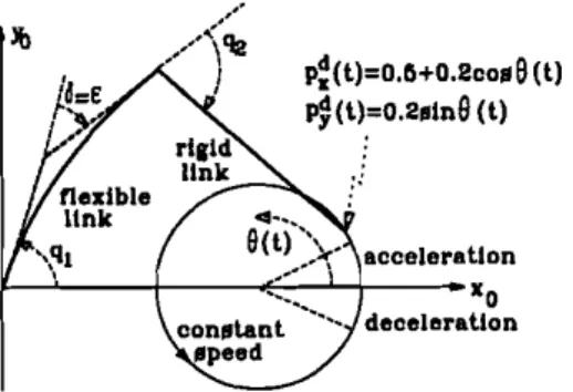
0; that is, the inverse ofA pp, required in (3.15), is avoided. 5. Simulationresults

The proposed two-time-scale control is tested by digital simulation of a planar two-link manipulator shown in Fig. 2. Performances of non-collocated control based on calculated and estimated parameters are compared with each other and with a simple collocated control based on the rigidity assumption. 5.1. Manipulator and trajectory descriptions

The manipulator shown in Fig. 2 consists of two links, the first one being flexible. The links have lengths 0·5 m and masses 10 kg each. The effective inertias and damping coefficients of the actuators are 6·35 kgmZ _{and 2·12 N m s}

for the first joint, and 1·30 kg m'' and 0·43 N ms for the second joint.

The flexible link is modelled by a second-order bulk approximation consist-ing of two sublinks havconsist-ing length 0·25 m each. Assumconsist-ing that an actuator is placed at the second joint, the mass of the flexible link is distributed between the sublinks as 2 kg and 8 kg respectively. The spring constant and the damping

p:(tl=o.6+o.2co.e (tl ~(tl=o.2.ln9(tl :: acceleration X_o deceleration

Figure 2. Simulated flexible manipulator and the desired trajectory.

coefficient of the fictitious joint are assumed to be Ks= 400 N m and Kd= 0 N m s respectively. Note that the numerical value of Ks is large enough to justify a singularly perturbed model.

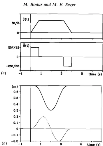
The trajectory to be followed by the end-point is a circular path in the plane of the manipulator with radius 0·2 m and centred at (0,5 m, 0) as also shown in Fig. 2. It is to be traced in 4 s starting from the point (0,7 rn, 0), with an angular velocity and acceleration as specified in Fig. 3(a). Corresponding displacements of the end-point in cartesian coordinates are shown in Fig. 3(b). This trajectory is chosen particularly to demonstrate the effectiveness of the proposed control scheme under large inertial variations along the path.

The simulations are performed for a discrete model of the manipulator corresponding to a sampling period of T = 0·005 s. That is, the manipulator parameters are updated (either by calculation or by estimation) once every 0·005 s, as well as the value of the control input. The Runge-Kutta method with a step size of h

=

0·001 s is used for numerical integration of the manipulator equations during each sampling period.

5.2. Collocated control

The collocated control is designed for a rigid model given as

Aqqij(t) + Bqqq(t) + cq= 'q(t) (5.1)

which is obtained from (2.1) by neglecting the flexible modes. Discretization of (5.1) yields

T- ZAqq!:i.Zqk

+

T- 1Bqq!:i.qk

+

cq= 'k (5.2)

which is of the form of (3.2). The control required to track a desired trajectory

qt specified in joint coordinates has the same structure as 1:k in (3.10), and is

given by

'k = T- zAqq!:i.Zqt

+

T-1Bqq!:i.qt

+

cq

+

Kq1ek_1

+

KqZek-z (5.3)

where ek

=

qt - qk' Hence, the choice

Kql

=

T-Z[A qq

+

(A qq

+

TBqq)(Zql

+

l)]}

(5.4)

Kqz

=

T- 1Bqq

+

T-Z(A qq

+

TBqq)(ZqZ - I)

M/:~

\

21111'/32

Set)

I

0

U

-2lll1/32

(a) -I 3 II limo (a)

...

(m) 0.6 0.11 0.4 0.3' 0.2 0.1 0 -0.1 (b) -0.2-I _{3 II limo (a)}

Figure 3. Description of the desired trajectory: (a) angular speed and acceleration along the desired trajectory specified in Fig. 2; (b) desired end-point displacements (p~: solid,

P~: dotted).

results in an error equation

ek

+

Zqlek_1

+

Zqzek-z

=

0 (5.5)

whose poles can be assigned arbitrarily.

Note that the control law in (5.3) involves only the measurement of the angular displacements of the actual joints, and is, therefore, much simpler to implement than the non-collocated control based on a two-time-scale model.

In the simulations, _{Kql and Kqz in (5.4) are selected to place the poles of the} error equation in (5.5) at z

=

(1

+

20T)-1

=

0·8333, which corresponds to continuous-time poles at s

=

-20. In the first simulation, parameters Aqq, Bqq and cq are calculated at every discretization step using the generalized

d'Alern-bert formulation along the actual trajectory qk assuming rigid links. The desired trajectory

qi

is obtained from the specified cartesian trajectory

pi

using inverse kinematic relations with Ok = 6.0k= O. The simulation results shown in Fig. 4

indicate approximately 15% maximum error in the x-direction and 29% max-imum error in the y-direction relative to the radius of the circular path. The static error in the y-direction is attributed to the deflection of the flexible link due to gravity. A compensation of this static torque is expected to improve the performance of the collocated control. To verify this, a second simulation is

(m) . , . - - . - - - , 0.011 0.03 0.02 0.01 limo (a) 3 o.+--!---.---.----r--...---.--,----! -I (a) II limo (a) 3 (dog) -2 -2.11 -3 -3.11 -4 -4.11 -II -11.11 -6' -6.11+--+-=--,....--.---.---.----,---,.-~:-:' (b) -I

Figure 4. Response to collocated control: (a) tracking error (e~: solid, e~: dotted); (b)

fictitious joint displacement.

carried out, in which the desired trajectory q~ is generated from p~ assuming quasi-constant deflections

b

k

=

K;lc o.The parameters Aqq , Bqq , cq and Coare

calculated from the measured values of qk and

{h

assuming /),.{h

=

O. The

simulation results shown in Fig. 5 indicate that the static error is eliminated, and the maximum tracking errors in the x- and y-directions are reduced to approximately 1% and 4% respectively.

5.3. Non-collocated two-time-scale control

A second group of simulations are performed to test the performance of the composite control law derived in §3. The feedback gains

K

1 and

K

₂ of the slow

control are chosen to place the eigenvalues of the slow subsystem at z

=

(1

+

20T)-1

=

0·8333, the same value used in simulation of the collocated control. The feedback gains

K

1 and

K

2 of the fast control are chosen to place

the fast poles at

z

=

(1

+

60n-1

=

0·6250, corresponding to continuous-time poles at s

=

-60, three times faster than the slow poles, to provide rapid decay of oscillations.

Simulation results with the manipulator parameters calculated along the desired trajectory are shown in Fig. 6. The results indicate that while the tracking errors are comparable with those in the case of collocated control with

(m) 0.004 0.002 0 '.

..

.

,' -0.002 .. -0.004 ~ :': i -0.006 ::_.: -: :: .: (a) -0.006-1 3 6 time (_) (de,) -3 -4 -6 -8 -7 (b) -1 3 6 time (_)

Figure5. Response to collocated control with static compensation: (a) tracking error (e~:

solid. e~: dotted); (b) fictitious joint displacement.

static compensation (approximately 2% maximum error in both directions), a major advantage of the composite control is observed to be the elimination of the long-lasting oscillations at the completion of the trajectory.

Finally, the simulations are repeated with the parameters estimated as described in §4. In the estimation algorithm, zero-mean triangular signals with amplitudes '0 = 50 N m and periods 3T and 5T are added to the input torques to excite all modes of the manipulator. The forget factor is taken to be y= 0·8, and the initial value of the matrix Pk in (4.6)' to be Po= 201. During

estimation, Pk is reset to Po whenever the diagonal elements exceeded 50. The

results shown in Fig. 7 indicate that the self-tuning control is as good as the one based on calculated parameters, with the added advantage of being implement-able on-line.

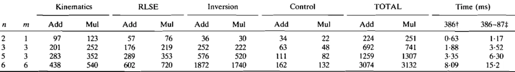
We conclude our discussion with a few comments on the computational complexity of the proposed control scheme. Table 1 provides expressions for the total number of additions and multiplications involved at each discrete time step in terms of the number of actual and fictitious joints. Table 2 shows the corresponding numerical values as well as the CPU times (including data transfer between memory and registers) for two different processors. As can be observed from Table 2, the proposed adaptive non-collocated control scheme

II time (~) 3

~

~\

r

'I. '. :'lA IV

-

V....·

_.'

...

:

..

:

\

..

_'..' V 0.001 (m) 0.003 0.002 o -0.001 -0.002 -0.003 -0.004 (a) -1 (dell) -2 -3 -4 -II -8 -7 (b) -1 3 II time (~)

Figure 6. Response to non-collocated control based on calculated parameters: (a) tracking

error(e~:solid, e~: dotted); (b) fictitious joint displacement.

based on a two-time-scale model is suitable for on-line control of even relatively sophisticated manipulators with up to six flexible links.

6. Conclusions

A two-time-scale adaptive control scheme is proposed for motion control of flexible manipulators. The self-tuning controller is based on a cartesian-space dynamic model of the manipulator obtained by approximating the flexible links with rigid sublinks connected at fictitious joints, and an estimation algorithm used to obtain the parameters of this model.

Bulk approximation of flexible links yields a model which is not much more complicated to control than a rigid one, but which includes a reasonable representation of the vibrational modes. Although modelling accuracy can be improved by a finer division of the flexible link into sub links, this increases the order of the dynamic equations, and hence, the amount of computations involved in generating the control. Besides, not all the vibrational modes may be controlled by a limited number of actuators. This corresponds to a case where m> n, so that (3.8) may not be solvable for arbitrary

.2

₁and

.2

_{2 ,}

Working with a dynamic model in cartesian coordinates has the advantage

3 6 time (s) 3 6 Ume (s) (m) 0.004 0.002 0 -0.002

-.

.:.\ -0.004 -0.006 -0.006 _~

_i

-0.01 .' (u) -I (del) -2 -3 -4 -6 -6 -7 (b) -I

Figure 7. Response to adaptive non-collocated control: (c) tracking error (e~: solid, ep': dotted); (b) fictitious joint displacement.

Computation Additions Multiplications

Kinematics RLSE Inversion Control law Total n2_{+30n +31m + nm} 3·5n2_+3·5m2_{+7·5n+8·5m+tnm+2} n 3+n2_{+m 3+m}2_+3n2m_+3m2n_+2nm n2_{+ l3n +2m +nm} { n3+6·5n 2_{+50·5n + m 3+4·5m}2₊ 41·5m +3n2m +3m2n + Ilnm +2 n2 _{+39n+ 39m + nm} 4n2_+4m2_{+lln+12m+8nm+6} n 3 +n+ m 3+m+3n2m+3m 2n n2 _{+6n +4m + nm} n3+6n2_{+57n+m 3+4m}2_{+56m +} 3n 3m +3m2n + 10nm +6 Table1. Operations count for adaptive non-collocated control.

that a desired trajectory can be specified directly in the task space. This eliminates the need for calculating the desired joint displacements using inverse kinematic relations, which is not only computationally tedious but also inaccu-rate during fast motions of the manipulator.

Implementing the control using an on-line estimation scheme makes the control structure independent of the coordinate system in which the manipulator is modelled. However, it requires that the end-point position and the deflections of the flexible links be measurable for feedback purposes and that the computa-tions involved be done in reasonable time. A simplified model like the one in

TOTAL

Kinematics RLSE Inversion Control

n m Add Mul Add Mul Add Mul Add Mul

2 1 97 123 57 76 36 30 34 22

3 3 201 252 176 219 252 222 63 48

5 3 283 352 289 353 576 520 111 82

6 6 438 540 602 720 1872 1740 162 132

t 80386 (30MHz) processor with32bit signed integer arithmetic.

+

80386-87 (30MHz) processor with 64 bit floating point arithmetic.

Table 2. Number of operations and CPU times.

Add 224 692 1259 3074 Mul 251 741 1307 3132 Time (ms) 386t 386-87:1: 0·63 1·\7 1·88 3·52 3·35 6·30 8·09 15·2 {;

-;;:.

'"

8

_;::

~

-.s;,

';:!, ~ 5:

""

:3 I::

::::-~

;>;-:3

'"

;::

.;:;.

I::

s-C ;;: VI W W

§4 helps reduce the computational effort without causing any significant degradation of the controller performance.

Appendix

Derivation of the two-time-scale model Defining the state variables

Xlk

=

Pk, XZk

=

T-1tJ.Pk' Zlk

=

T-ZEb ZZk

=

T-ZtJ.Ek (A 1) Equations (2.7) can be written in state space form

[j

o

o

I

o

o ]

[tJ.X

lk]

[0

TAp, tJ.XZk = 0

o

tJ.Z 1k 0 TAu _{tJ.Z Zk} 0 T -TBpp

o

o

o

o

o

-TK;

where K;

=

TZKs •Using (3.4), (A 2)can be manipulated into

(A 2) [ tJ. Xlk]

[0

tJ.XZk _ 0 tJ.zlk - 0 tJ.Z Zk 0 T -TEppBpp

o

-E,pBpp

o

-TEp,K;

o

-EuK;

Equations (A 3) reveal that incremental changes tJ.Xlk and tJ.XZk are of the order of T, indicating a slow (quasi-constant) behaviour of Xlk and XZb while Zlk and ZZk consist of both slow and fast components. Decomposing the state variables into slow and fast components as

and attributing the incremental changes tJ.Z ik to their fast components, the slow components of Zik can be solved from the last two equations in (A 3) with T

=

0 as

[

~lkJ

_ZZk

(A 4)

Replacing Zlk and ZZk in the first two equations in (A3) with Zlk and ZZk

above and using the relations in (3.4), we get

[

~~lkJ

=

T[0

~XZk 0 (AS)

which, together with (A 4), describes the slow subsystem. The fast dynamics are readily obtained from the last two equations in (A 3), by setting T

=

0, as

(A6)

Finally, rewriting (A 4)-(A 6) in terms of the slow and fast components of the original variables Pk and lib we get (3.2), (3.3) and (3.5).

REFERENCES

BALESTRINO, A., DEMARIA, G. and SCIAVICCO, L., 1983, An adaptive model following control

for robot manipulators. Transactions of ASME Journal of Dynamic Systems and

Measurement Control, lOS, 143-151.

BOOK, W. J., 1984, Recursive Lagrangian dynamics of flexible manipulator arms. International

Journal of Robotics Research, 3, 87-101; 1985, New concepts in lightweight arms, Proceedings of the 2nd International Symposium on Robotics Research, (Cambridge,

Mass: MIT Press), pp 203-205.

CANNON, R. H., JR, and SCHMITZ, E., 1984, Precise control of flexible manipulators.

Proceedings of the lst International Symposium on Robotics Research, (Cambridge,

Mass: MIT Press), pp. 841-861.

CRAIG, J. J., 1988, Adaptive Control of Mechanical Manipulators, (New York:

Addison-Wes-ley).

<;ETINKUT, S., SICILIANO, B., and BOOK, W. J., 1986, Symbolic modeling and dynamic analysis

of flexible manipulators. Proceedings of the IEEE International Conference Systems

Man Cybernetics, Atlanta, pp. 798-803.

FREUND, E., 1982, Fast nonlinear control with arbitrary pole placement for industrial robots and manipulators. International Journal of Robotics Research,1,65-78.

GOODWIN, G. C., and SIN,K. S. 1984, Adaptive Filtering Prediction and Control (Englewood

Cliffs, NJ: Prentice Hall).

JUDO, P. R., and FALKENBURG, D. R., 1985, Dynamics of nonrigid articulated robot linkages.

IEEE Transactions on Automatic Control, 30, 499-302.

KING, J. 0., GOURISHANKAR, V. G., and RINK, R. E., 1990, Composite pseudolink end-point

control of flexible manipulators. IEEE Transactions on Systems Man Cybernetics, 20,

969-977.

KOlVO, A. J., 1985, Self tuning manipulator control in Cartesian base coordinate system.

Transactions of ASME Journal of Dynamic Systems Measurement and Control, 107,

316-323; 1989,Fundamentals for Control of Robot Manipulators, (New York: Wiley).

KOlVO, A. J., and Guo, T., 1983, Adaptive linear controller for robotic manipulator. IEEE

Transactions on Automatic Control, 28, 162-170.

KOKOTOVIC, P. V., 1984, Applications of singular perturbation techniques to control problems.

SIAM Review, 26, 501-550.

LEE, C. S. G., and LEE, B. H., 1984, Resolved motion adaptive control for mechanical

manipulators. Transactions of ASME Journal of Dynamic Systems Measurement and

Control, 106, 134-142.

LEE, C. S. G., LEE, B. H., and NIGAM, R., 1983. Development of the generalized d'Alembert

equations of motion for mechanical manipulators. Proceedings of the 22nd Conference

on Decision and Control, San Antonio, Texas, pp, 1205-1210.

LUH, J. S., WALKER, M. W., and PAUL, R. P. C. 1980, Resolved acceleration control of

mechanical manipulators. IEEE Transactions on Automatic Control, 25, 468-474.

NEMIR, D. C, KOIVO, A. J., and KASHYAP R. L., 1988, Pseudolinks and the self-tuning control of a nonrigid link mechanism. IEEE Transactions on Systems, Man and Cybernetics, 18, 40-48.

SICILIANO, B., and BOOK, W. J., 1988, A singular perturbation approach to control of lightweight flexible manipulators. International Journal of Robotics Research, 7, 79-90.

SLOTlNE, J. J. E., 1985,The robust control of robot manipulators. International Journal of Robotics Research, 4, 49-64.

SOUISSI, R., and KOIVO, A. J., 1987, Design of self-tuning controllers for high-speed manipulators. Proceedings of the IEEE International Conference on Systems, Man and Cybernetics, Alexandria, Virginia, pp. 897-902.

TAKEGAKI, M., and ARIMOTO, S., 1981, A new feedback method for dynamic control of manipulation. Transactions on the ASME Journal of Dynamics Systems Measurement and Control, 102, 119-125.

VICKER, J. J., DENAVIT, J., and HARTENBERG, R. S., 1964, An iterative method for the displacement analysis of spatial mechanisms. Journal of Applied Mechanics, 26,

309-314.