Full Terms & Conditions of access and use can be found at
https://www.tandfonline.com/action/journalInformation?journalCode=tmpm20
Maritime Policy & Management
The flagship journal of international shipping and port research
ISSN: (Print) (Online) Journal homepage: https://www.tandfonline.com/loi/tmpm20
Forecasting COVID-19 impact on RWI/ISL container
throughput index by using SARIMA models
Kaan Koyuncu , Leyla Tavacioğlu , Neslihan Gökmen & Umut Çelen Arican
To cite this article: Kaan Koyuncu , Leyla Tavacioğlu , Neslihan Gökmen & Umut Çelen Arican (2021): Forecasting COVID-19 impact on RWI/ISL container throughput index by using SARIMA models, Maritime Policy & Management, DOI: 10.1080/03088839.2021.1876937
To link to this article: https://doi.org/10.1080/03088839.2021.1876937
Published online: 24 Jan 2021.
Submit your article to this journal
Article views: 257
View related articles
View Crossmark data
Forecasting COVID-19 impact on RWI/ISL container throughput
index by using SARIMA models
Kaan Koyuncua, Leyla Tavacioğlub, Neslihan Gökmenc and Umut Çelen Aricand
aTransportation Service Programme, Marina and Yacht Management, Muğla Sıtkı Koçman University, Muğla,
Turkey; bMaritime Faculty, Basic Sciences Department, Istanbul Technical University, İstanbul, Turkey; cMaritime
Faculty, Basic Sciences Department, Istanbul Technical University, Istanbul Turkey; dArkas Line, Project Manager of
ARMA, Istanbul, Turkey
ABSTRACT
Maritime operators are facing their biggest challenge called Coronavirus (COVID-19) since the 2008 financial crisis. As part of the measures taken by the countries against the virus, the domino effect started with the breaks in the interconnected supply chain, like the spider web. The main purpose of this study is modeling the Institute of Shipping Economics and Logistics (ISL) and the Leibniz-Institut für Wirtschaftsforschung (RWI) Container Throughput Index with the time series, to reveal the relationship between the short-term forecast results and the COVID-19 seen in the first months of 2020. The deep effect of COVID-19 on maritime trade is investigated by forecasting the RWI/ISL Container Throughput Index in 89 major interna-tional container ports, including and excluding seasonal variations. The modeling process of the Seasonal Autoregressive Integrated Moving Average (SARIMA) and Exponential Smoothing State Space Model (ETS) is explained. To evaluate SARIMA and ETS models’ performance, informa-tion criteria, and error measurements are calculated and compared. SARIMA model is found as more suitable model than ETS forecasting seasonally and working-day adjusted and original RWI/ISL. The results indicated that the SARIMA model is suitable and efficient for the forecast-ing of RWI/ISL. Three months’ forecastforecast-ing results are showed that the decrease will continue.
KEYWORDS
COVID-19; forecasting; maritime trade; containers; SARIMA; RWI/ISL
1. Introduction
COVID-19, called the new type of coronavirus, has spread unexpectedly all over the world. As a result, the World Health Organization (WHO) was declared an ‘Emergency’ on 30 January 2020. On 11 March 2020, the latest situation was announced as ‘Pandemic.’
COVID-19 outbreak has had a huge impact on global supply chains. Pandya, Herbert-Burns, and Kobayashi (2011) define maritime trade as a kind of trade that entails the transportation of commodities including containers through the sea.
There is no doubt that the huge effects of COVID-19 on the maritime trade sector are felt by China than any other country in the world since it is the epicenter of the pandemic. The negative effects of COVID-19 on the shipping companies increase day by day. One of the negative impacts is the decrease in the number of containers shipped especially from China to other countries around the world (McKibbin and Fernando 2020).
CONTACT Leyla Tavacioğlu [email protected] Maritime Faculty, Basic Sciences Department, Istanbul Technical University, Tuzla, İstanbul, Turkey
MARITIME POLICY & MANAGEMENT https://doi.org/10.1080/03088839.2021.1876937
© 2021 Informa UK Limited, trading as Taylor & Francis Group
!l
Routledge
~ ~ Taylor & Francis Group I "'> Check for updates I
Recently, there is a great shortage of containers in many of the developing countries of Africa that majorly depended on maritime trade with China. Such a trend is causing an economic crisis which gives other potential traders with economic advantage to increase the price of containers because of the prevailing high demand. According to the information from the Sea Intelligence, many of the Chinese ships carrying containers are currently undergoing blank sailings. Additionally, there are a good number of ships that have been quarantined at the ports of China since the emergence of COVID-19 hence cannot move to the required destinations to transport containers. While this act is done to stop the spread of COVID-19, maritime trade is being affected negatively (McKibbin and Fernando 2020). On the same note, since new policies have been introduced to limit the use of ships to travel to other parts of the traders, many of the traders who are using the sea routes cannot now transport their goods conveniently to other markets because of the existing quarantine.
The emergence of COVID-19 has contributed greatly to the congestion that is currently seen in China has the world’s seven busiest container ports and Asian-European ports. In China, such congestion at the port has caused an imbalance in the local and international markets. The containers which were being used in carrying perishable goods to other countries are now lying in heaps at the ports. This means that the Maritime trade is suffering a great blow since the required products cannot reach other countries due to the existing quarantine. So, a good number of products which were being transported through the maritime channels are getting destroyed due to the fear of people to travel in other parts of the world which are already affected by COVID-19.
According to Alphaliner Reports data, there was a significant drop in all Chinese coastal ports (including Hong Kong). With the advent of COVID 19, due to deferred deliveries in China, a drop of −15.8% was observed in total container products only in February. The total volume of contain-ers handled at Chinese coastal ports decreased by 10.1% in the first two months of 2020 when compared to the same period in 2019. Not only this but also full-year volumes can record negative growth rates for the first time since 1970. These recorded figures are under the record level of −6.1% which was recorded in the financial crisis in 2009.
According to the survey by Alphaliner, which is related to Asia-Northern Europe services, 33 sailings of January have been canceled. This means that 46% of departures planned to act on the route were affected by the situation. According to this data, carrier schedules and customer announcements show that 17 sailings more stayed in blank in February. From this scope, it is thought capacity decrements over the eight weeks from Chinese New Year may reach nearly 700,000 TEU.
Dyna Reports, which makes research on the subject, states that this open chaos situation and uncertainty will have serious effects on container shipping. Some formations, such as 2 M Alliance, reacted by making some arbitrary cancellations. After the chain reaction of the situation, almost half of Europe-Far East sailings formations canceled their calendars during February, with the end of Chinese New Year. Not only these but also the Ocean Alliance formation also announced that it made seven additional cancellations in February, some of which belonged to the April calendar.
After all the developments, the inactive containership reached a record level again and thus, 402 ships for 2.46 M teu were not operated in the first two months of 2020. RWI/ISL index involves the data on container throughput in 89 international ports which is continuously collected as part of the ISL Monthly Container Port Monitor, and which generates nearly 60% of global container throughput (Institute of Shipping Economics and Logistics 2020). From this aspect, RWI/ISL index and international trade are expected to be highly correlated.
Therefore, this article explores the results for the short-term forecasting of the RWI/ISL index, considering seasonal variations of the Box-Jenkins and ETS models. First, Box-Jenkins and ETS modeling methodology is explained. Second, time series models are proposed for the original and seasonal index. Finally, the effectiveness of the models developed for the indexes is evaluated using
appropriate performance metrics and 3-month forecasting results are explained after diagnostic analysis.
2. Methodology
Monthly RWI/ISL data are collected from January 2007 to February 2020 were used to make 3-month forecasts for original series and seasonally and working-day adjusted series. Due to the first month of 2020 is a turn point in the time series, the period January 2007 to December 2019 is used to forecast the first three months of the year 2020. The validity of the model is provided by using this period as a training data set. R programming language is used in the modeling stage. The proposed RWI/ISL index forecasting methodology includes the following stages: analysis of time series data, test for stationarity, model identification and estimation, diagnostic checking, evalua-tion, and forecasting.
2.1. Analysis of time-series data
Time series are sets of well-defined data sets that are collected at variable time intervals as well as at equal time intervals. Autocorrelation functions are examined to determine whether the series is time series. The ACF function (Autocorrelation Function) and PACF (Partial Autocorrelation Function) show the linear dependence of the values in the time series with the past values (lag). If the autocorrelation functions show significant peaks with a continuous pattern that repeats over the total length of the lags, it is reasonable to consider the seasonality of the series.
2.2. Test for stationarity
The concept of stationary has a great priority of the time series analysis. The concept of stationarity is expressed as the mean and variance of a time series is constant and the covariance between the two values of the series depends not only on the examined time but only on the difference between the two-time series. In order to apply the time series models, the series should be adjusted from the trend and seasonality (time-invariant). Correlograms (ACF and PACF graphs) can show a stationarity pattern or a unit root with significant lags. A more subjective way to evaluate stationarity is using (augmented) Dickey-Fuller (ADF) test statistics (Dickey and Fuller 1979). The null hypothesis is that the series have a unit root. The alternative hypothesis is that the time series is stationary (or trend-stationary).
2.3. Model identification and estimation
ARIMA models are also referred to as Box-Jenkins Models in the literature. ARIMA model consists of autoregressive and moving average processes that are integrated with the same degree. Box- Jenkins method, basically an attempt is made to create a combination of two different methods (Autoregression and Moving Average). The letter ‘I’ (integrated) in ARIMA showed that the modeling time series was converted to a stationary time series. The models that makeup with this method are divided into non-seasonal and seasonal types. The non-seasonal Box-Jenkins models are generally expressed as ARIMA p; d; qð ÞHere, p is the degree of autoregression (AR) model, d is the number of differentiation operations, and q is the degree of the moving average (MA) model. The basic approach in Box-Jenkins models is that the present value of the examined variable is based on the combination of the weighted sum of past values and random shocks. Whether the series is stationary and whether it has a seasonal effect is decisive in the selection of the model. Therefore, firstly, the properties of the time series are revealed, and an appropriate model is tried to be found. The Box-Jenkins method uses a four-step iterative approach to determine a suitable model among all model combinations. These steps are; determination, parameter estimates,
diagnostic tests, and prospective prediction stages. If the specified model is not sufficient, the process is repeated using another model created to develop the original model. This process is repeated until a satisfactory model is obtained. It is important to examine the autoregressive (AR) and moving average (MA) processes that form the ARIMA model (Box and Jenkins 1976). ARIMA model’s formula is given below:
φ Bð ÞÑdy tð Þ ¼θ Bð Þε tð Þ (1) with φ Bð Þ ¼1 φ1B1 . . . φpBp θ Bð Þ ¼1 þ θ1B1þ . . . þθ qBq Ñdy tð Þ ¼ð1 BÞdx tð Þ
In the formula, BK is the lag operator of K; Ñ is the difference operator;φ Bð Þis the autoregressive
polynomial of p with autoregressive parameter of φ1;φ2; . . . ;φp; θ Bð Þindicated moving average polynomial of q, as the moving average parameter displayed as θ1;θ2; . . . ;θq; stationary time series
reflects as Ñdx tð Þ; ε tð Þbrings out as independent white noise sequences and fits the Gaussian distribution.
Time series often contain cyclical properties (seasonal effects) where seasonal variation is used to eliminate seasonal effects. These sorts of models are acknowledged as SARIMA models. Thus, two general types are given for ARIMA models: non-seasonal ARIMA and multiplication seasonal ARIMA (SARIMA). SARIMA models are usually denoted as SARIMA p; d; qð Þ �ðP; D; QÞSP is the
order of the seasonal autoregressive (SAR) part. D is the order of the seasonal differencing. Q is the order of the seasonal moving-average (SMA) process. S is the length of the seasonal cycle (Xinxiang, Zhou, and Huijuan 2017). SARIMA model’s formula is as follows:
φ Bð Þ; BS�ÑdÑDSy tð Þ ¼θ Bð Þ# BS�ε tð Þ (2) with
; BS�¼1 ;1BS . . . ;PBPS # BS�¼1 þ #1BSþ . . . þ #QBQS
ÑDSy tð Þ ¼ 1 BS�Dx tð Þ
In the formula, B, Ñ,y tð Þ, φ Bð Þ, θ Bð Þand ε tð Þare consistent with the ARIMA model.; Bð SÞindicates
seasonal autoregressive polynomial as ;1; ;; . . . ; ;P acts as the seasonal autoregressive parameter. #ðBS) stands for seasonal moving average polynomial as #
1; #; . . . ; #Q acts as seasonal mobbing
average parameter; ÑDS signifies the seasonal difference which goes through the D order (Xinxiang, Zhou, and Huijuan 2017).
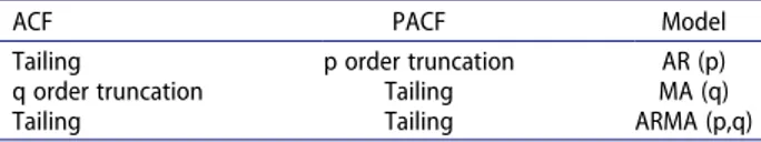
ACF and PACF are calculated to perform model identification of the time series. In general, we can predict the possible values of model order p; q; P and Q by observing the ACF and PACF graphs, and then choose the most suitable model order by Akaike’s information criterion (AIC), Bayes’ information criterion (BIC) (Yang, Zheng, and Zhang 2017). The criterion of model order is shown in Table 1.
For the SARIMA model, besides using the low-order ARMA model to accomplish short-term correlation effects, the ARMA model with periodic steps is also used to distinguish from the
seasonal effects. After examining the order of the model, the parameters can be estimated. The methods used in this stage are the least-squares that can be acquired with the statistical software.
Another prediction method used as an alternative to ARIMA models is Exponential Smoothing State Space Model (ETS). ETS model is usually a three-character string identifying method using the framework terminology of Hyndman et al. (2002). The first letter states the error type (‘A,’ ‘M,’ or ‘Z’); the second letter states the trend type (‘N,’”A,””M,” or ‘Z’); and the third letter denotes the season type (‘N,’”A,””M,” or ‘Z’). In all cases, ‘N’ = none, ‘A’ = additive, ‘M’ = multiplicative, and ‘Z’ = automatically selected. For example, ‘ANN’ is a simple exponential smoothing with additive errors, ‘MAM’ is multiplicative Holt-Winters’ method with multiplicative errors. ETS equations for ANN are given as follows:
lt ¼αPtþð1 αÞQt (3)
μt ¼lt 1 lt¼lt 1þαεt
where l denotes the series level at time t, Pt and Qt vary according to which of the cells the methods
belong, and α is constant. For ANN Pt¼yt and Qt¼lt 1 are considered. MAM are obtained by
replacing εt and μtεt in the above equations. If there are zeros or negative values in the data, the
multiplicative error models are not suitable. Due to having a subclass (ANN, MAM, etc.), ETS models share a consistent set of functionality with those models, which can make it easier to work with. In addition, confidence intervals for forecasts can be computed by using ETS and it supports concentrating the initial state out of the likelihood function (Hyndman et al. 2002).
2.4. Diagnostic checking
To measure the validity of the model, the residual distribution of the model should be tested. The tool, which is thought to be suitable for examining white noise is an autocorrelogram (ACF) (Farhan and Ong 2018). In addition to visual investigation of residuals, the Box-Ljung statistics can be engaged for a more objective interpreted analysis. If the p-value of the statistics is greater than the significance level, it can be considered that the residuals have a random sequence, which demonstrate that the information has been fully extracted by the model. In the contrary case, extracted information is not adequate and the model needs to be improved (Ljung and Box 1978).
2.5. Evaluation and forecasting
Two penalty function statistics are used in model selection: AIC and BIC (Akaike 1974; Schwarz
1978). Information criteria approach such as AIC combines two concepts into one framework: an error control procedure that controls the prediction error and the maximum likelihood principle that serves as a measure of compliance. The AIC or BIC for a model is usually written in the form
2logL þ kp
½ �where L is the likelihood function,p is the number of parameters in the model, and k
Table 1. The ARMA model order criterion (Yang, Zheng, and Zhang 2017).
ACF PACF Model
Tailing p order truncation AR (p)
q order truncation Tailing MA (q)
is 2 for AIC and log nð Þfor BIC (Reddy et al. 2017). The procedure to select the most appropriate model is based on choosing the model with minimum AIC and BIC.
Mean absolute percentage error (MAPE) and root mean square error (RMSE) are calculated to evaluate forecasting error and the accuracy of the forecast (Chase 2013). MAPE is to some extent dependent on the scale; for example, estimating very low values or the size of the measurement can easily be inflated to an integer such as one or two. Therefore, it is best to use a series (MAPE and RMSE) of measures to assess the accuracy of the estimate. Root mean square error is an absolute measure of error that squares deviations to prevent positive and negative deviations from cancelling each other. When comparing methods this measure helps us by overestimating large errors. The formula for calculating the RMSE is given below:
RMSE ¼ ffiffiffiffiffiffiffiffiffiffiffiffiffiffiffiffiffiffiffiffiffiffiffiffiffiffiffiffiffiffiffiffiffiffiffiffiffiffiffiffi Pn t¼1 y tð Þ ycð Þt � �2 n v u u t (4) where y tð Þis the actual value of a point for given time period t, n is the total number of fitted points, and ycð Þt is the fitted forecast value for the time period t. Mean absolute percent error is a relative measure of error that uses absolute values to prevent positive and negative errors from cancelling each other and uses relative errors to enable you to compare the predictive accuracy between time series models.
The formula for calculating MAPE:
MAPE ¼100 n Xn t¼1 y tð Þ ycð Þt y tð Þ � � � � � � � � � � (5)
where y tð Þis the actual value of a point for given time period t; n is the total number of fitted points, and ycð Þt is the fitted forecast value for the time period t (Agrawal, Muchahary, and Tripathi 2018).
The forecasting stage consists of five steps. Forecasting steps are as follows:
Rearrange ARIMA equation so y tð Þis on left hand side. Rewrite equation by replacing tby T þ h. On the right-hand side, replace future observations by their forecasts, future errors by zero, and past errors by corresponding residuals. Start with h = 1. Repeat for h = 2,3, . . . Similar steps are performed for ETS models.
3. Results
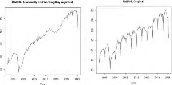
In the period from January 2007 to February 2020, RWI/ISL is shown in Figure 1(a,b). Considering the seasonal influence of the RWI/ISL series, the SARIMA and ETS models are used to predict the RWI/ISL.
Seasonally and working day adjusted RWI/ISL has a non-stationary trend with decreasing averages (Figure 1(a,b)). The ADF test was used to investigate the stationarity of the series. To solve the problem of autocorrelation, it is stated that the lags of the dependent variable were added to the right of the equation and the ADF test was called the test applied to the new model created (Said and Dickey 1984). As can be seen in Table 2, the null hypothesis is rejected at the 0.05 significance level for original RWI/ISL and first-order difference seasonally and working day adjusted. When the original RWI/ISL plot (Figure 1(b)) is examined, it is obvious that a seasonal difference should be taken.
The ACF and PACF plots of seasonally and working day adjusted RWI/ISL and original RWI/ ISL are examined and the degrees of seasonal and non-seasonal autoregression (AR) and moving average (MA) processes are determined. ACF plots are used to determine the degree of MA, PACF plots are used to determine the degree of AR. It can be seen that the linear decline of ACF is slow and that there is a significant meaningful block in PACF for seasonally and working day adjusted
RWI/ISL (Figure 2). Considering that the first difference in the series is also stationary, the SARIMA (2,1,3) (2,0,1)12 model is chosen as the appropriate model. The selected model is verified to be
appropriate using the stepwise model selection method.
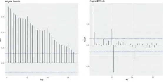
For the original RWI/ISL, the SARIMA (2,0,2) (2,1,2)12 model is chosen as the appropriate
model, considering that the linear decrease in ACF is slow and there is an increase in some lags. Moreover, the first two important blocks in the PACF are considered when determining the model (Figure 3). The selected model is verified to be appropriate using the stepwise model selection method.
Figure 1. Time series plots of seasonally and working day adjusted RWI/ISL (a) and original RWI/ISL (b).
Table 2. ADF test results for evaluating stationarity.
RWI/ISL Original Seasonally and working day adjusted Seasonally and working day adjusted (1st order difference)
ADF p-value <0.001 0.337 <0.001
Figure 2. Autocorrelation and partial autocorrelation functions of seasonally and working day adjusted RWI/ISL. 0 § 0 "" lil 12
RW1nsL Seasonally and Working Day Adjusted
/"--
·-'
/
vV
,0011 Zll111 }Dl~ 20,i 10-m T1m<>RWI/ISL Sensonaly ancl Wotk.ng Oa~ ~
100 -,,.. ,
...
,,..
/I
;;()18 20,0--- --- --
n
--,oo-LLLLILLJ...LIJ.lJ.l_LJ__LJ_Ll.l.LLULU...U.J...l.J...lililLLLl._ " RWUISL Or1glnal ~
rrrfn
~ 0 0 0 "'(i
i;i 0 ~ g :>008 1010 ;>012 ;>01• limeRWUISL S."""'81y ond Wod<ng Doy Ad;u,lod
,.,.
,
...
,,,
_
" ;.
The final models and estimates for RWI/ISL indexes are presented in Table 3. It can be observed from the table that the significant parameters at a level of significance of 0.05 and 0.10 is shown in bold. Both models are found significant.
Another forecasting model used in series with trend and seasonal effects is the ETS model. In order to find the most suitable model, ETS is also used. The smoothing parameter is chosen as alpha 0.89 for seasonally and working day adjusted RWI/ISL. The smoothing parameter is chosen as alpha 0.53, beta 0.17, gamma 0.19, and phi 0.81 for original RWI/ISL. The comparison of ETS and SARIMA with model prediction outcome and performance evaluation is shown in Table 4. According to the results, the SARIMA models, where the information criterion and error values are lower, are found more suitable models for forecasting RWI/ISL.
Examining the residual plots helps you to evaluate if the least-squares assumptions are met. If these assumptions are met, the least squares estimations will produce with a minimum variance
Figure 3. Autocorrelation and partial autocorrelation functions of original RWI/ISL.
Table 3. The summary output of time series analysis using SARIMA model.
Seasonally and
working day adjusted
RWI/ISL Estimate Standard Error t p Original RWI/ISL Estimate Standard Error t p AR (1) 0.8174 0.0107 76.3925 <0.001 AR (1) 1.7414 0.2331 74.7061 <0.001 AR (2) −0.0487 0.0097 −5.0206 <0.001 AR (2) −0.7813 0.2180 −3.5839 <0.001 MA (1) −1.1689 0.0925 −126.368 <0.001 MA (1) −1.1129 0.2283 −48.7473 <0.001 MA (2) 0.5557 0.1278 4.3482 <0.001 MA (2) 0.4400 0.0785 5.6051 <0.001 MA (3) −0.0162 0.0950 −0.1705 0.864 SAR (1) −0.7308 0.4434 −1.6482 0.101 SAR (1) −0.2100 0.0176 −11.9318 <0.001 SAR (2) −0.145 0.179 −0.8101 0.419 SAR (2) −0.0506 0.0043 −11.7674 <0.001 SMA (1) 0.0934 0.4419 0.2114 0.832 SMA (1) 0.2363 0.1015 2.3281 0.021 SMA (2) −0.3702 0.2459 −1.5055 0.134 Drift 0.2459 0.0475 5.1768 <0.001
Table 4. SARIMA and ETS models’ prediction outcome and performance evaluation. Seasonally and working day
adjusted
RWI/ISL AIC BIC RMSE MAPE
Original
RWI/ISL AIC BIC RMSE MAPE
SARIMA(2,1,3)(2,0,1)12 630.49 657.99 1.69 1.17 SARIMA(2,0,2)(2,1,2)12 with drift 626.66 656.5 1.79 1.38 ETS 978.50 996.87 1.69 1.19 ETS 1026.17 1081.30 1.83 1.51 Ongiod RWVISL 075
-...
....
....
·
·
1T
··
·~
_
..._
~,-,,
,.
,', i, Log,...
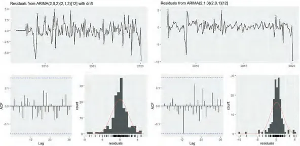
(Yang, Zheng, and Zhang 2017). The residual plots for original RWI/ISL and seasonally and working day adjusted RWI/ISL are shown in Figure 4(a,b). The top line plot is a chart of all residuals are ordered and can be used to find a non-random error of time-related effects. This plot shows that residuals are unrelated and distributed randomly. In the plots on the bottom left, ACF and PACF are examined to see if they are almost zero. According to Figure 4(a,b), the residuals are almost zero and the white noise can be considered, so the model has a better predictive effect. On the residual histogram plots of the bottom right, a long tail on one side can show a skewed distribution. If one or two bars are far from the others, these points may be outliers. When
Figure 4(a,b) are examined, it is seen that there is no outlier problem and the residuals are distributed randomly. So, there is no heteroscedasticity or changing variance problem.
Moreover, according to ARCH model, the model is found non-significant (p ¼ 0:32 for origi-nal,p > 0:05). Therefore, our SARIMA model has met the assumptions criteria; thus, we can continue to forecast the RWL-ISL index by SARIMA model.
As the last step, when model diagnostics are examined based on a statistical test, it is seen that the residuals are randomly distributed (Ljung-Box test p=0.831 for seasonally and working day adjusted and p=0.905 for original; p > 0:05).
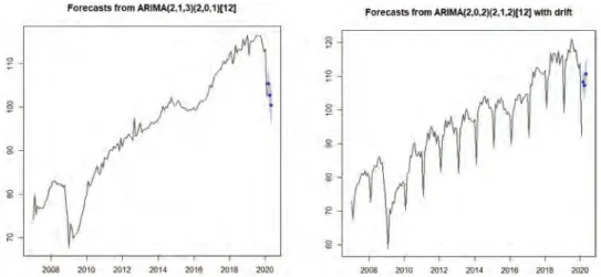
Since model performance and diagnostics are controlled, the forecasting results can be exam-ined. 3-month (March, April, and May) forecasting is utilized with the SARIMA models. The data belongs to February are also shown in Table 5 for the comparison. The predicted values are significant as they fall within the 95% confidence interval.
When the forecasting results are shown with graphs, the original RWI/ISL series increased after April, while the seasonally and working day adjusted RWI/ISL series decreased after March (Figure 5(a,b)). This decline that became more evident when the series is seasonally,
Figure 4. Residual plots to check diagnostics original RWI/ISL (a), seasonally and working day adjusted RWI/ISL (b).
Table 5. The forecast values and 95% confidence intervals of RWI/ISL.
Seasonally and working day adjusted 95% Confidence Intervals Original 95% Confidence Intervals
Month Forecast Values Lower Upper Forecast Values Lower Upper
February 102.5 - - 92.4 -
-March 105.4607 102.0449 108.8765 108.24 104.45 112.02
April 102.7471 98.6760 106.8182 107.29 102.81 111.76
May 100.4215 95.3849 105.4581 110.61 105.31 115.92
Rosi<luOIS from ARIMA(2,0,2X2, 1,2H12} woth ~<lft
~i,
-...
00·,..
-ao-,,. JO·b
I
il1i1
[
I
I IIii
;
20 • < .. II
I
I '11'1II
11111 I' 8 ,o--01·••
..
Lag.
'°"' 4Jllllll . . . •U~II..
l'Hiduals'
.
Residuals from ARIMA(2,1,3X2,0, 1H12J
S·
•·
-•· ,..
.,.
~,-,\••
Lag JD•,..
' moand working-day adjusted, it can be associated with the global epidemic (COVID-19) seen all over the world.
4. Validity of the model
In the period from January 2007 to December 2019, RWI/ISL is used for checking the forecast results and validity of the model. Considering the seasonal influence of the RWI/ISL series, the SARIMA and ETS models are used to predict the RWI/ISL. According to the ADF test, the null hypothesis is rejected at the 0.05 significance level for original RWI/ISL and first-order difference seasonally and working day adjusted. When the original RWI/ISL plot (Figure 1(b)) is examined, it is obvious that a seasonal difference should be taken.
The ACF and PACF plots of seasonally and working day adjusted RWI/ISL and original RWI/ ISL are examined and the degrees of seasonal and non-seasonal autoregression (AR) and moving average (MA) processes are determined. Considering that the first difference in the series is also stationary, the SARIMA (2,1,2) (2,0,0)12 model is chosen as the appropriate model. For the original
RWI/ISL, the SARIMA (1,0,1) (2,1,1)12 model is chosen as the appropriate model, considering that
the linear decrease in ACF is slow and there is an increase in some lags. The selected models are verified to be appropriate using the stepwise model selection method. 3-month (January, February, March) forecasting is utilized and the results are shown in Table 6. Actual values remain within the 95% confidence interval estimated by SARIMA. New year celebrations were delayed in many parts of China to stop the spread of the epidemic across the country. Due to strict measures were taken for Covid-19, trade has come to a stagnation point. After the chain reaction of the situation, almost half of the vessels that operate on the Europe-Far East trade line canceled their February calendars.
Figure 5. Forecasting of seasonally and working day adjusted RWI/ISL (a), original RWI/ISL (b).
Table 6. The forecast values and 95% confidence intervals of RWI/ISL for validity of the model. Seasonally and working day
adjusted
95% Confidence
Intervals Original
95% Confidence Intervals
Month Real Value Forecast Values Lower Upper Real Value Forecast Values Lower Upper
January 113.3 113.6 110.6 116.6 115.1 113.2 109.6 116.9 Febuary 106.9 113.9 110.5 117.4 94.6 101.4 96.9 105.9 March 109.7 113.2 109.2 117.3 109.4 114.1 109.0 119.2
Fe recasts rrom ARIMA(2, 1 ,3ll2,0, 1 l[12] Forecasts from ARIMA(2.0,2l(2, 1,2)[12] With dr11t
11
.
This led to a great fluctuation of trade volumes and indices in February. This dramatic fluctuation shows the seriousness of the situation and how it affects the trade worldwide. For this reason, February forecast is found slightly out of the 95% confidence interval. As a result, it can be said that the forecasts with the SARIMA model are reliable and valid.
5. Discussion
It is true that the emergence of COVID-19 does not only have immediate effects on the shipping industry but also has future effects. When model comparisons are determined, the MAPE and RMSEA are calculated below 10% indicates excellent performance. The reason for this is that the COVID-19 effect that occurred since January and this variability is included in the models. With the announcement of real values in the coming months, it can be observed that performance will increase even more by updating the model. The fact that COVID-19 has led to the shortage of containers shipped to many countries in the world will have a future negative impact which will not be easy to reverse. One such future impact will be an economic crisis which will increase the demand prices of the maritime trade commodities due to shortage. Such a crisis is likely to affected countries which were manufacturing and transporting containers as well those which were receiv-ing and usreceiv-ing containers in various business activities.
6. Future effects of COVID-19 on maritime trade and shipping of containers 6.1. Optimists approach
Some people who are optimistic about the sector think that after the virus file is closed, everything will be restored thanks to the improvements expected from the countries. Nevertheless, many countries will make some radical decisions due to these long-lasting supply problems and trade problems. Changes may occur in operations in some countries other than China.
There are still some positive effects for the container shipping area. Customer Perspective: The first was the collapse of the bunker surcharges lines that gained from the increase in fuel prices in January. As a result, less payment is made for fuel. The other positive side for the liner perspective was the discipline that the COVID-19 carrier elements showed in the voyages that remained empty. Thus, the discipline that the carrier elements showed throughout the process due to the high virus level in China. There was no dump in freight rates.
After the restrictions disappear, shipping companies will stand up with a strong recovery and companies will be in a hurry to replenish their stocks (Smith 2020).
6.2. Pessimist approach
According to the Public Health England report, COVID-19 epidemic will continue till 2021 spring and could cause to 8 million people being hospitalized (The Guardian 2020). If COVID-19 spreads all over the world with a high effect and there will be no vaccine, the maritime sector crisis may continue for a long time unfortunately.
According to BIMCO, the speed and severity of the outbreak are increasing unpredictably, and this unpredictable situation makes it impossible to predict about the industry. Moody’s stated that the negative situation in the maritime trade sectors will continue in the next 18 months (Watkins
2020).
The Alliance announced new cancellations on the Asia-Europe trade line in March. Until the first week of April and May, a total of 15 cancellations are on the agenda. These cancellations, including 15 ships, were calculated as 235,000 TEU in total.
New COVID-19 pandemic circumstances will cause carriers to realize extra ad hoc capacity cuts. In addition to the capacity decreasing that planned in the early stages of this year, The Alliance and
2 M announced some huge capacity cuttings within the Asia-Europe trade lines. This will cause the carriers to face a sharp decrease in their westbound volumes and this hard impact will be felt instantly.
The contraction in this capacity shows a dramatic decrease in trade volumes to Italy and Spain after the spread of the virus in the European region. These countries have gone down in history as the countries most affected by the outbreak compared to others. On the other hand, India has been struggling with a deadlock for the past 3 weeks. Some shipping lines have announced that they have cancelled their journey in this direction.
After these recent developments, important data were obtained from China and India, which have half the world’s population. Lockdown situations in these countries affected most of the sectors. With the declaration of lockdown, Italy and Spain, which are members of the European Union, are expected to continue the global downward trend increasingly.
Finally, the disconnection in the maritime trade as far as the transport of containers to other countries is concerned will lead to the death of formal and legal maritime trade. This will pave the way for the emergence of unscrupulous business individuals and organizations using maritime channels to further their ill agenda in the transportation of containers. It must be understood that such a situation is quite disastrous especially to the developing countries which eventually be exploited to a greater deal due to their state of vulnerability.
7. Conclusion
This study aims to examine the relationship between the short-term estimate of the RWI/ISL Container Throughput Index and COVID-19 using time series models. The model is estimated by using SARIMA and ETS models. The models developed have been shown to be accurate and appropriate for forecasting seasonal variation. In light of these forecasts, when we compared the results, which obtained from previous year’s March, April, and May with the RSW/ISL index data, it was seen that COVID-19 had a negative effect on the market from the moment it was first seen, and it is predicted that the decline will continue until May.
With this decreasing determination, it is expected that the momentum of the container transportation sector, which its trend has increased rapidly within the year, will be lost due to the restrictions in production and trade. It is thought that with the breaks in the interconnected supply chain, such as spider web, people around the world may experience some serious problems in reaching their commercial and personal needs. Nevertheless, liquidity concerns in the industry will also affect carriers due to stagnation caused by the COVID-19 outbreak. This problem, which will cause serious losses in profitability levels, will create problems on carriers as well. Especially, the balance sheets of companies on some container lines may receive permanent damage due to losses.
Disclosure statement
No potential conflict of interest was reported by the authors.
References
Agrawal, R. K., F. Muchahary, and M. M. Tripathi. 2018. “Long Term Load Forecasting with Hourly Predictions
Based on Long-short-term-memory Networks.” In 2018 IEEE Texas Power and Energy Conference (TPEC), 1–6.
IEEE. doi: 10.1109/TPEC.2018.8312088.
Akaike, H. 1974. “A New Look at the Statistical Model Identification.” IEEE Transactions on Automatic Control 19
(6): 716–723. doi:10.1109/TAC.1974.1100705.
Box, G. E. P., and G. M. Jenkins. 1976. Time Series Analysis: Forecasting and Control San Francisco. Calif: Holden-
Chase, C. W. 2013. Demand-driven Forecasting: A Structured Approach to Forecasting. New Jersey: John Wiley & Sons.
Dickey, D. A., and W. A. Fuller. 1979. “Distribution of the Estimators for Autoregressive Time Series with a Unit
Root.” Journal of the American Statistical Association 74 (366a): 427–431. doi:10.1080/01621459.1979.10482531.
Farhan, J., and G. P. Ong. 2018. “Forecasting Seasonal Container Throughput at International Ports Using SARIMA
Models.” Maritime Economics & Logistics 20 (1): 131–148. doi:10.1057/mel.2016.13.
The Guardian. 2020. “UK Coronavirus Crisis ‘To Last until Spring 2021 and Could See 7.9m Hospitalised’.” https://
www.theguardian.com/world/2020/mar/15/uk-coronavirus-crisis-to-last-until-spring-2021-and-could-see-79m- hospitalised
Hyndman, R. J., A. B. Koehler, R. D. Snyder, and S. Grose. 2002. “A State Space Framework for Automatic
Forecasting Using Exponential Smoothing Methods.” International Journal of Forecasting 18 (3): 439–454. doi:10.1016/S0169-2070(01)00110-8.
Institute of Shipping Economics and Logistics. 2020. “RWI/ISL Container Throughput Index.” https://www.isl.org/
en/containerindex
Ljung, G. M., and G. E. P. Box. 1978. “On a Measure of Lack of Fit in Time Series Models.” Biometrika 65 (2):
297–303. doi:10.1093/biomet/65.2.297.
McKibbin, W. J., and R. Fernando. 2020. “The Global Macroeconomic Impacts of COVID-19: Seven Scenarios.”
SSRN Electronic Journal. doi:10.2139/ssrn.3547729.
Pandya, A. A., R. Herbert-Burns, and J. Kobayashi. 2011. Maritime Commerce and Security: The Indian Ocean.
Washington: Henry L. Stimson Center.
Reddy, J. C. R., T. Ganesh, M. Venkateswaran, and P. Reddy. 2017. “Forecasting of Monthly Mean Rainfall in Coastal
Andhra.” International Journal of Statistics and Applications 7 (4): 197–204. doi:10.5923/j.statistics.20170704.01.
Said, E., and D. Dickey. 1984. “Testing for Unit Roots in Autoregressive-moving Average Models of Unknown
Order.” Biometrika 71 (3): 599–607. doi:10.1093/biomet/71.3.599.
Schwarz, G. 1978. “Estimating the Dimension of a Model.” The Annals of Statistics 6 (2): 461–464. doi:10.1214/aos/
1176344136.
Smith, J. 2020. “Coronavirus Impact Seen Prolonging U.S. Freight Slump.” https://www.wsj.com/articles/corona
virus-impact-seen-prolonging-u-s-freight-slump-11582832476
Watkins, E. 2020. “BIMCO Revises 2020 Forecasts on Coronavirus Concerns.” https://lloydslist.maritimeintelligence.
informa.com/LL1131574/BIMCO-revises-2020-forecasts-on-coronavirus-concerns
Xinxiang, Z., B. Zhou, and F. Huijuan. 2017. “A Comparison Study of Outpatient Visits Forecasting Effect between
ARIMA with Seasonal Index and SARIMA.” In 2017 International Conference on Progress in Informatics and
Computing (PIC), 362–366. IEEE. doi: 10.1109/PIC.2017.8359573.
Yang, Y., H. Zheng, and R. Zhang. 2017. “Prediction and Analysis of Aircraft Failure Rate Based on SARIMA Model.”
In 2017 2nd IEEE International Conference on Computational Intelligence and Applications (ICCIA), 567–571.