BORNOVA / İZMİR NOVEMBER 2016
YAŞAR UNIVERSITY
GRADUATE SCHOOL OF NATURAL AND APPLIED SCIENCES
MASTER THESIS
A HYBRID FLOW SHOP SCHEDULING PROBLEM IN
INK PRODUCTION
AYLİN AKÇALI
THESIS ADVISOR: ASST. PROF. ADALET ÖNER
MASTER OF INDUSTRIAL ENGINEERING
v
ABSTRACT
A HYBRID FLOW SHOP SCHEDULING PROBLEM IN INK PRODUCTION
AKÇALI, Aylin MSc in Industrial Engineering Supervisor: Asst. Prof. Dr. Adalet ÖNER
November 2016
This study concerns with Hybrid Flow Shop Scheduling (HFS) problem and its real world application in a factory that produces ink and related special paints. There are many variations of HFS depending on the machine environment, process (job) characteristics and objective function. This study focus on a special variation that includes the constraints of machine blocking, sequence-dependent setup times, limited buffers and machine eligibility and having an objective of minimizing makespan. This variation is imposed by the properties of real production system in the factory. An original MIP model has been formulated to get the optimal solutions for small scale instances of the problem. The outcomes have been reported for a set of test problems. However, since HFS problems are classified as NP-hard, mathematical models are incapable of solving medium and large instances of the problem which may be seen in real world applications. Therefore, it is necessary to study heuristic methods. Different construction heuristics are used to generate initial schedule such as Shortest Processing Time and Longest Processing Time and their variants. To improve the initial solution, Simulated Annealing and Tabu Search methods are utilized with different control parameters. The performances of the heuristics have been evaluated on small scale problems by comparing with the optimal solutions obtained with MIP model. Finally, large scale problems have been generated to imitate real scheduling problems in the factory and their solutions have been reported.
Key Words: Hybrid Flow Shop Scheduling, Mathematical Modelling, Heuristics, Machine Blocking, Sequence-dependent Setup Times, Limited Buffers, Machine Eligibility
vii
ÖZ
MÜREKKEP ÜRETİMİNDE ESNEK AKIŞ TİPİ ÇİZELGELEME PROBLEMİ
Aylin AKÇALI
Yüksek Lisans, Endüstri Mühendisliği Bölümü
Tez Danışmanı: Yrd. Doç. Dr. Adalet ÖNER Kasım 2016
Bu çalışmada, Esnek Akış Tipi (EAT) çizelgeleme problemi ve çözüm yöntemleri ile bunların mürekkep üreten bir fabrikadaki gerçek çizelgeleme problemi üzerindeki uygulaması ele alınmıştır. Makine yapısına, işlem özelliklerine ve amaç fonksiyonuna göre EAT çizelgeleme probleminin birçok varyasyonu vardır. Bu çalışmada fabrikadaki gerçek üretim sürecinin dikte ettiği özel bir varyasyon üzerinde durulmuştur. Buna göre modelde makine bloklama, sıra bağımlı hazırlık süreleri, sınırlı kuyruk ve makine uygunluğu kısıtları bulunmalıdır. Amaç fonksiyonu da en son bitirilen işin tamamlanma zamanını en küçük değerine düşürmektir. Bu problemi çözebilmek için bir Karmaşık Tam Sayılı Doğrusal Programlama modeli geliştirildi. Bu model kullanılarak küçük ölçekli problemlerin en iyi çözümleri gösterildi. Ancak EAT çizelgeleme problemlerinin NP-zor karmaşıklık sınıfında olduğu bilindiğinden, bu model orta ve büyük ölçekli problemleri çözmede yetersiz kalmaktadır. Bundan dolayı, genellikle sezgisel yöntemlerin kullanması gerekliliği ortaya çıkar. Bu çalışmada farklı sezgisel yöntemler üzerinde durulmuştur. İlk çizelgeyi üretmek için, En Kısa İşlem Süresi, En Uzun İşlem Süresi ve bunların varyasyonları olan farklı kurucu sezgiseller kullanıldı. İlk çizelgeyi geliştirmek için ise, Tabu Arama (TA) ve Benzetimli Tavlama (BT) meta sezgiselleri farklı kontrol parametreleri ile kullanıldı. Sezgisel yöntemlerin performansı, küçük ölçekli problemlerde, daha önce matematiksel model ile elde edilen en iyi çözümlerle karşılaştırılarak değerlendirildi. Son olarak, fabrikadaki gerçek çizelgeleme problem örnek alınarak, büyük ölçekli problemler oluşturuldu ve bunların sonuçları rapor edildi.
Anahtar Kelimeler: Esnek Akış Tipi Çizelgeleme Problemi, Matematiksel Modelleme, Sezgisel Yöntemler, Makine Bloklama, Sıraya Bağlı Kurulum Süresi.
ix
ACKNOWLEDGEMENTS
I would like to thank to my supervisor Asst. Prof. Dr. Adalet ÖNER for his support, valuable contributions, and advices. He believed in me to complete my thesis successfully.
I would like to thank to Prof. Dr. Levent KANDİLLER and Assoc. Prof. Dr. Raif Serkan ALBAYRAK for their support, advices, and valuable contributions. Most of all they believed in me.
I also want to state from the heart thank my family, and friends for supporting and believe in me. Especially I would like to thank to Emre DALOĞLU who always stand by me, believe in me and encourage me.
Aylin AKÇALI İzmir, 2016
xi
TEXT OF OATH
I declare and honestly confirm that my study, titled “Hybrid Flow Shop Scheduling Problem” and presented as a Master’s Thesis, has been written without applying to any assistance inconsistent with scientific ethics and traditions, that all sources from which I have benefited are listed in the bibliography, and that I have benefited from these sources by means of making references.
Aylin Akçalı Signature ……….. December 28, 2016
xiii TABLE OF CONTENTS ABSTRACT ... v ÖZ ... vii ACKNOWLEDGEMENTS ... ix TEXT OF OATH ... xi
TABLE OF CONTENTS ... xiii
LIST OF FIGURES ... xv
LIST OF TABLES ... xvii
ABBREVIATIONS AND SYMBOLS ... xix
CHAPTER ONE INTRODUCTION ... 1
CHAPTER TWO PROBLEM DEFINITION ... 3
Basic Concepts & Notations ... 3
2.1.1. Machine Environment ... 4
2.1.2. Process (Job) Characteristics ... 8
2.1.3. Performance Measures (Objective Functions) ... 10
Case Study: Ink Production ... 12
CHAPTER THREE LITERATURE SURVEY ... 17
CHAPTER FOUR MATHEMATICAL MODEL ... 23
Basic Hybrid Flow Shop Model (M0) ... 26
Hybrid Flow Shop Model With Machine Blocking (M1) ... 31
Hybrid Flow Shop Model With Machine Blocking And Sequence Dependent Setup Times (M2) ... 32
Hybrid Flow Shop Model With Machine Blocking, Sequence Dependent Setup Times And Limited Buffer (M3) ... 33
Hybrid Flow Shop Model With Machine Blocking, Sequence Dependent Setup Times, Limited Buffers And Machine Eligibility (M4) ... 34
Model Verification ... 35
xiv
CHAPTER FIVE HEURISTIC METHODS ... 45
Construction Heuristics – Dispatching Rules ... 45
Improvement Heuristics ... 46
5.2.1. Simulated Annealing ... 47
5.2.2. Tabu Search ... 49
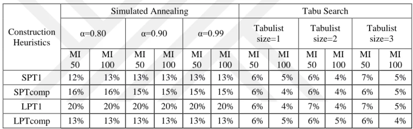
Solving Small Scale HFS Problems ... 50
Solving Large Scale Generic HFS Problems ... 51
Solving Real HFS Problem ... 55
CHAPTER SIX CONCLUSION & DISCUSSIONS ... 63
REFERENCES ... 65
CURRICULUM VITAE ... 77
APPENDIX 1 – Model Structures Of Studies In The Literature ... 79
APPENDIX 2 – Solution Methodologies Used In The Studies In The Literature ... 87
APPENDIX 3 – Solutions Of Problem Sets For Verification Of Mathematical Model ... 91
APPENDIX 4 – Solutions Of Small Scale Problems By Utilizing Heuristics ... 101
APPENDIX 5 – Solutions Of Large Scale Problems By Utilizing Heuristics ... 105
APPENDIX 6 – Solutions Of Real Problems By Utilizing Heuristics ... 116
APPENDIX 7 – Solutions Of Large Scale Generic Test Problems With Coupling Of Heuristics... 129
xv
LIST OF FIGURES
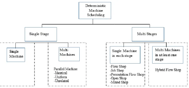
Figure 1. Basic Classification of Machine Scheduling Problems 2
Figure 2. A Sample Schedule for Flow Shop 5
Figure 3. A Sample Schedule for Permutation Flow Shop 5
Figure 4. A Sample Schedule for Job Shop 6
Figure 5. A Sample Schedule for Open Shop 6
Figure 6. A Sample Schedule for Mixed Shop 7
Figure 7. Process Flow in Hybrid Flow Shop Problem 8
Figure 8. Example Precedence Constraint 9
Figure 9. Structure of DYO Ink's Production Line 13
Figure 10. Distribution of Machine Types in Literature 18 Figure 11. Distribution of Buffer Size in Literature 18 Figure 12. Distribution of Setup Time in Literature 19 Figure 13. Distribution of Performance Measures in Literature 19 Figure 14. Distribution of Solution Methodology in Literature 20 Figure 15. Distribution of Solution Methodologies in Literature 21 Figure 16. Solution of Problem 17 (Unlimited Buffer) 38 Figure 17. Solution of Problem 18 (Limited Buffer Size 0) 39 Figure 18. Solution of Problem 19 (Limited Buffer Size 1) 40
Figure 19. Structure of SA Algorithm 48
xvii
LIST OF TABLES
Table 1. Setup Time in DYO Ink's Production Line 13
Table 2. Machine Eligibility in DYO Ink's Production Line 14
Table 3. Buffer in DYO Ink's Production Line 14
Table 4. Machine Blocking in DYO Ink's Production Line 14 Table 5. Properties of Mathematical Models in Literature 20 Table 6. Number of Decision Variables in Model (M0) 29 Table 7. Number of Decision Variables in Modified Model (MM0) 30 Table 8. Comparison of Structure of Basic Model and Modified Basic Model 31 Table 9. Performance Comparison of Basic and Modified Basic Models 31 Table 10. Common Characteristics of Test Problems 35
Table 11. Summary of Test Problems 35
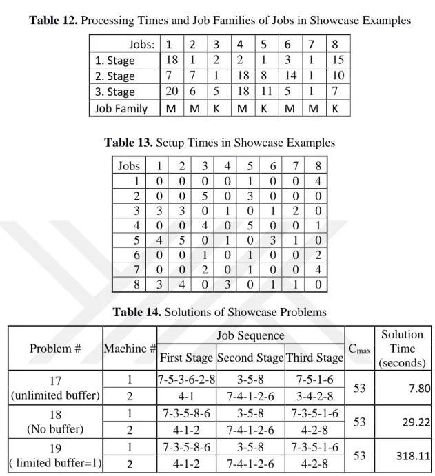
Table 12. Processing Times and Job Families of Jobs in Showcase Examples 37
Table 13. Setup Times in Showcase Examples 37
Table 14. Solutions of Showcase Problems 37
Table 15. Solution Times of Test Problems 41
Table 16. Common Characteristics of Supplementary Test Problems – Set 1 41 Table 17. Solution Times of Supplementary Test Problems – Set 1 41 Table 18. Common Characteristics of Supplementary Test Problems – Set 2 42 Table 19. Solution Times of Supplementary Test Problems – Set 2 43 Table 20. Denomination of Construction Algorithms 50 Table 21 . Number of Cases Where Heuristics Achieve Optimal Solutions 51 Table 22. Mean Percentage Deviations from Optimal Solutions 51 Table 23. Comparison of Real Scheduling Problem and Generic Test Problems 52 Table 24. Heuristics Control Parameters and Their Levels For Large Scale Problems 53
xviii
Table 25. Best Results of Heuristics Across Different Control Parameters with K=20 53 Table 26. Best Results of Heuristics Across Different Control Parameters with K=50 54 Table 27. Best Results of Heuristics Across Different Control Parameters with K=100 55 Table 28. Heuristics Control Parameters and Their Levels For Real Problems 56 Table 29. Best Results of Heuristics for Real HFS Problem Across Different Control
Parameters with K=50 56
Table 30. Best Results of Heuristics for Real HFS Problem Across Different Control
Parameters with K=75 57
Table 31. Best Results of Heuristics for Real HFS Problem Across Different Control
Parameters with K=100 57
Table 32. Effect of Coupling Configuration, K=50, Large Scale Generic Problems 59 Table 33. Effect of Coupling Configuration, K=100, Large Scale Generic Problems 60 Table 34. Effect of Coupling Configuration, K=50, Real Problem 61 Table 35. Effect of Coupling Configuration, K=100, Large Scale Real Problems 62
xix
ABBREVIATIONS AND SYMBOLS
ABBREVIATIONS:
HFS Hybrid Flow Shop
FFS Flexible Flow Shop
M0 Basic Hybrid Flow Shop Model
MM0 Modified Model
M1 Hybrid Flow Shop Model with Machine Blocking
M2 Hybrid Flow Shop Model with Machine Blocking and Sequence Dependent Setup Times
M3 Hybrid Flow Shop Model with Machine Blocking, Sequence Dependent Setup Times and Limited Buffer
M4 Hybrid Flow Shop Model with Machine Blocking, Sequence Dependent Setup Times, Limited Buffers and Machine Eligibility
TS Tabu Search
SA Simulated Annealing
SPT Shortest Processing Time
SPT1 Sorting jobs in ascending order according to their processing time in Stage-1
SPTcomp Sorting jobs in ascending order according to their total completion times
xx
LPT1 Sorting jobs in descending order according to their processing time in Stage-1
LPTcomp Sorting jobs in descending order according to their total completion times
SYMBOLS: 𝐶𝑚𝑎𝑥 Makespan i Processing stage j Machine in a stage k, l Jobs M Number of stages K Number of jobs
𝑚𝑖 Number of parallel machines in stage i
𝑝𝑖𝑘 Processing time for job k in stage i
𝑄 A large number
𝜀 A small number
𝑠𝑡𝑖𝑘 Starting time of job k at stage i.
𝑥𝑖𝑗𝑘 Job k is assigned to machine j in stage i
𝑦𝑖𝑘𝑙 Job k precedes job l at stage i
𝑠𝑖𝑘𝑙 Setup time for job l if job k is the immediately preceding job in sequence operation on the stage i
xxi
𝑏𝑞 Index for artificial stage corresponds to buffers
q Buffer
g Job Types
G Number of job types
𝑆𝑖 Set of machines in stage i
𝐹𝑖𝑔 Set of machines for job type g in stage i
1
CHAPTER ONE
INTRODUCTION
Scheduling is a decision-making process that is used on a regular basis in many manufacturing and service industries. This form of decision-making plays an important role in procurement and production, in transportation & distribution, and in information processing & communication. Scheduling functions in company rely on mathematical techniques and heuristic methods to allocate limited resources to the activities that have to be conducted. The performance measures for scheduling may have different forms such as minimizing completion time of the activities, minimizing the number of tardy activities etc.
Scheduling problems can be classified depending on various factors. For example, they may be divided into two basic classes depending on the nature of the scheduling system:
Static problems: All the jobs are ready for processing at the beginning of the scheduling period, i.e., ready times are zero.
Dynamic problems: New jobs are added to the system as time goes on, i.e., nonzero ready times.
If uncertainty is considered, there is another classification of scheduling problems: Deterministic problems: All the quantities required to define the problem are
known in advance and fixed (number of jobs, processing times, due dates etc.). Uncertain problems: All or some quantities required to define the problem have
random components.
In manufacturing systems, orders are translated into the jobs which have to be processed on the machines with given order or sequence. Delay, preemption, unexpected events have to be considered because they may impact on the schedule. Manufacturing systems can be characterized by several factors, such as number of machines, configuration of machines, material flow system, and so on. Because of these characteristics, many variations of scheduling problems can be defined. Basic classification of machine scheduling problem is shown in Figure 1.
2
Figure 1. Basic Classification of Machine Scheduling Problems
This study is concerned with a specific variation of scheduling problems, namely, hybrid flow shop scheduling problem (HFS). The technical characteristics of the problem are given in detail in the next chapter. The inspiration came from a real production system at DYO Inks Company that is located in Manisa, Turkey. The company produces ink and related special paints. One of the production lines is designed in the form of HFS.
The rest of this thesis is organized as follows. Basic concepts, notations and detailed definition of HFS are given in Chapter 2. This chapter also includes the description of real production line at the company. Chapter 3 covers literature review of HFS scheduling problem. A mathematical model is formulated and its solutions for sample problems are presented in Chapter 4. Heuristic solution methods are discussed in Chapter 5. Finally, Chapter 6 is devoted to results and conclusion.
3
CHAPTER TWO
PROBLEM DEFINITION
Production scheduling briefly refers to finding best sequence and timing for processing a set of jobs through one or several machines. Practical and technological constraints such as flow pattern of the jobs through machines lead to different production models which are called flow shop, job shop, open shop, etc. In order to present a detailed definition of HFS, basic concepts and notation in scheduling are reviewed first.
Basic Concepts & Notations
The number of jobs is denoted by K, the number of stages denoted by M and the number of machines is denoted by 𝑁. The subscripts “k” and “l” refer to distinct jobs while subscripts “i” and “j” refer to stages and machines respectively. The following input data are associated with job k:
Processing time is represented by 𝒑𝒋𝒌 and it represent the processing time of job
k on machine j.
Release date is represented by 𝒓𝒌 and it is also known as ready time. It is time
the job arrives at the system.
Due date is symbolized by 𝒅𝒌 and it represents the committed shipping and completion date. After due date, if job k is not completed, a penalty cost will be incurred.
Weight is denoted by 𝒘𝒌 and it is priority factor, reflecting the importance of job k relative to other jobs in the system.
Starting time is represented by 𝒔𝒕𝒋𝒌 and it refers to job k starts its processing on
machine j.
Completion time is denoted by 𝑪𝒋𝒌 and it refers job k is completed on machine
j.
There are many variations of machine scheduling problem depending on the machine environment, process (job) characteristics and objective. In literature, the taxonomy of scheduling problems is described by triplet 𝜶/𝜷/𝜸 (Graham et. Al, 1979). The first symbol 𝜶 represent machine environment. The symbol 𝜷 represents the
4
characteristics of processes (jobs) which refers to practical & technological constraints and assumptions. The symbol 𝜸 represents the objective function or performance measure of the problem.
2.1.1. Machine Environment
The first symbol 𝜶 represent machine environment with two entries in the form of 𝜶𝟏𝜶𝟐. Depending on the values of these two entries, possible machine environments
can be described as follows.
If 𝜶𝟏= 𝜶𝟐= 1, then it indicates single machine problem which is the simplest of all possible machine environments. If there are more than one machine, then the environment is defined as 𝜶𝟐 = 𝒏 where n indicates the number of machines. It implies that we have a multi-machine problem. In this situation, it assumed that the machines configured in parallel. If there is only one operation to be conducted on the jobs, and if any machine can perform the operation, then the problem is subdivided into three different environments.
Identical machines in parallel (𝜶𝟏= 𝑷 𝒂𝒏𝒅 𝜶𝟐= 𝒏) ∶ (Pn) : There are n identical machines and a job can be processed on any one of the machines. Then processing time of a job 𝒑𝒋𝒌 can be simplified into 𝒑𝒌 since the processing time of a job is the same on any one of the machine.
Uniform machines in parallel (𝜶𝟏 = 𝑸 𝒂𝒏𝒅 𝜶𝟐= 𝒏) ∶ (Qn) : There are n machines in parallel with different speeds. Let 𝒗𝒋 represent the speed of the machine, then the processing time of a job 𝒑𝒋𝒌 = 𝒑𝒌⁄ . 𝒗𝒋
Unrelated machines in parallel (𝜶𝟏 = 𝑹 𝒂𝒏𝒅 𝜶𝟐 = 𝒏) ∶ (Rn) : There are n machines in parallel. The speeds of the machines are dependent on the jobs, such as machine j can process job k at speed 𝒗𝒋𝒌 . Thus the processing time of job k can be found as 𝒑𝒋𝒌= 𝒑𝒌⁄𝒗𝒋𝒌 .
On the other hand, if there are multiple operations to be conducted on the jobs, then the machines are assumed to be configured in “m” stages or blocks in series. It means that the jobs follow a flow pattern (route) through the machines. Depending on the flow pattern, different machine environments can be defined as follows:
5
Flow Shop (𝜶𝟏= 𝑭 𝒂𝒏𝒅 𝜶𝟐 = 𝒏) ∶ (Fn) : There are n machines in series in the order of the operations. Each job should be processed on each one of the machines. Each job has the same flow pattern.
Permutation Flow Shop (𝜶𝟏= 𝑭 𝒂𝒏𝒅 𝜶𝟐 = 𝒏) ∶ (Fn/permu) : There are
n machines in series in the order of the operations. Each job should be
processed on each one of the machines. Each job has the same flow pattern. Additionally, each machine has the same sequence of jobs. In other words, a permutation of jobs is applied to all machines. The problem here is to find an optimal sequence (permutation), applicable to all machines with respect to some performance measures.
𝑀4 𝑀3 𝑀2 𝑀1 𝐽1 𝐽1 𝐽1 𝐽1 𝐽2 𝐽2 𝐽2 𝐽2 𝐽3 𝐽3 𝐽3 𝐽3 𝐽4 𝐽4 𝐽4 𝐽4 𝑀4 𝑀3 𝑀2 𝑀1 𝐽1 𝐽1 𝐽1 𝐽1 𝐽2 𝐽2 𝐽2 𝐽2 𝐽3 𝐽3 𝐽3 𝐽3 𝐽4 𝐽4 𝐽4 𝐽4
Figure 2. A Sample Schedule for Flow Shop
6
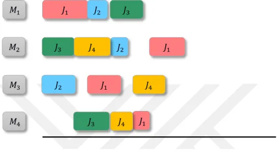
Job Shop (𝜶𝟏= 𝑱 𝒂𝒏𝒅 𝜶𝟐 = 𝒏) ∶ (Jn) : There are n machines in series in the order of the operations. There are k jobs. Each job may not need to be processed on each one of the machines, however each job has to be processed more than one machine and the order does not have to be the same. It means, each job has unique processing sequence.
Open Shop (𝜶𝟏 = 𝑶 𝒂𝒏𝒅 𝜶𝟐= 𝒏) ∶ (On) : There are n machines in series in the order of the operations. There are k jobs. Each job should be processed on each one of the machines and the order does not have to be the same. It means, any ordering will do.
𝑀4 𝑀3 𝑀2 𝑀1 𝐽1 𝐽1 𝐽1 𝐽1 𝐽2 𝐽2 𝐽2 𝐽3 𝐽3 𝐽3 𝐽4 𝐽4 𝐽4 𝑀4 𝑀3 𝑀2 𝑀1 𝐽1 𝐽1 𝐽1 𝐽1 𝐽2 𝐽2 𝐽2 𝐽2 𝐽3 𝐽3 𝐽3 𝐽3 𝐽4 𝐽4 𝐽4 𝐽4
Figure 4. A Sample Schedule for Job Shop
7
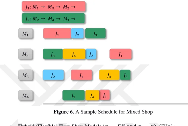
Mixed Shop (𝜶𝟏 = 𝑿 𝒂𝒏𝒅 𝜶𝟐= 𝒏) ∶ (Xn) : There is a subset of jobs and this gives fixed processing path which is specified. Jobs which are out of this subset being scheduled in order to minimize the objective function.
Hybrid (Flexible) Flow Shop Models (𝜶𝟏= 𝑭𝑯 𝒂𝒏𝒅 𝜶𝟐= 𝒏): (FHn) :
A hybrid (flexible) flow shop is a combination of the flow shop and the parallel machine environments. Basic framework of HFS may be presented as follows:
o Manufacturing processes can be divided into “m” stages or blocks in series. o Each job has to be processed first at stage 1, then at stage 2, and so on. o Each stage has a number of machines in parallel. Different operating
characteristics of the machines define different variants of the problem. If the processing speeds of all machines are the same for a job in a stage, the machines are called identical otherwise they are called uniform. If machines have different processing speeds depending on the jobs, then they are called
unrelated.
o A job requires processing on only one machine in a stage. In a given stage, any machine or only a predetermined subset of machines can process the job (machine eligibility restrictions). Each case defines a different variant of the problem. 𝐽1: 𝑀1 → 𝑀3 → 𝑀2 → 𝑀4 𝑀4 𝑀3 𝑀2 𝑀1 𝐽1 𝐽1 𝐽1 𝐽1 𝐽2 𝐽2 𝐽2 𝐽3 𝐽3 𝐽3 𝐽4 𝐽4 𝐽4 𝐽3: 𝑀2 → 𝑀4 → 𝑀1 → 𝑀3 𝐽3
8
o Setup time may or may not incur between two successive jobs. Setup time may be constant or it may vary depending on the job sequence and/or machines. (sequence and/or machine dependent setup times)
o The queues between the various stages may have different structures. The system may have limited or unlimited buffer in between two successive stages. In other case, jobs may not allow to wait between stages (No wait) o The objective is generally minimizing makespan or total tardiness or total
completion time. There are also some other performance measures defined in literature.
.
Figure 7. Process Flow in Hybrid Flow Shop Problem
2.1.2. Process (Job) Characteristics
The symbol 𝜷 represents the characteristics of processes (jobs) which refers to practical & technological constraints and assumptions. Job characteristics may be listed as follows:
𝜷 = prmp presence of preemption.
Preemption is related to the priority of jobs. During execution of a job on a machine, for some reason, if it requires to interrupt the processing of that job before finishing the process and to start a new job immediately on that machine, then preemption occurs. There are different forms of preemption such as
preemptive-resume and preemptive-repeat.
9
Precedence constraints refer to some technological constraints which contain the sequence and dependence relations between jobs. A job often can start only after a given set of other jobs has been completed. For example, job 4 in Figure 8 cannot be processed until job 1 and job 2 are completed and also job 6 cannot be started until job 4 and job 5 are completed.
𝜷 = 𝒔𝒌𝒍 sequence dependent setup times
Machines often have to be reconfigured and be cleaned between jobs. It takes some time which is called setup time. If the length of setup times depends on the job just completed and on about to be started, then the setup time is sequence dependent. If there is a setup time between job k and next job l on machine j, then setup time is represented by 𝑠𝑗𝑘𝑙.
𝜷 = 𝒔𝒋 machine dependent setup times
If the length of setup times depends on the machine instead of sequence of the jobs, then the setup time is machine dependent.
𝜷= 𝑴𝒌 machine eligibility restrictions
Machine eligibility constraint is restriction of assignment. In other words, job k cannot be assigned machine j even if it is available. Job k can only be assigned to a machine which is a member of a specific subset of machines.
𝜷 = buffer , 𝜷 = block
During job processing, a queue may temporarily be formed before a machine. It requires a storage area before that machine. The size of the storage area determines the nature of the buffer. It may be zero, limited or unlimited. If the storage space between two machines is zero or limited and when the buffer is full, first machine cannot release the job which is completed and also cannot process other jobs. It leads to machine blocking.
1 2 3 4 5 6
10
𝜷 = no wait
Jobs are not allowed to wait between two successive machines. It is due to either no buffer space between two machines or a technological requirement that implies the jobs shouldn’t be waited between machines.
Workforce constraint emerges in different situations. For example, the number of workers may be less than the number of machines. In the other case, some machines may require some skill set to operate and the number of workers that have required specific skill set may be less than the number of those machines. Therefore, a worker may be responsible more than one machine. It implies that job
k would wait for processing on a machine until one of the operators become
available.
Routing constraint is relevant with the route that a job must follow through the system. The routing constraint specify the order of machines which a job must visit. This constraint applies especially when the jobs may skip some machines for processing.
2.1.3. Performance Measures (Objective Functions)
The symbol 𝜸 represents the objective. There are various basic objectives. Some of the best known basic objectives are explained below. In practice, overall objective is often expressed as a composite of several basic objectives.
Throughput
Throughput is equivalent output rate and it is desired to be maximized. It is frequently determined by the bottleneck machine. There is a several ways to achieve. First one is, the bottleneck machine is never idle and all jobs wait in queue of these machine. Second, if there are sequence dependent setup times on the bottleneck machine, then the scheduler has to sequence the jobs in such a way that the sum of setup times or the average setup times, is minimized.
Makespan
Makespan is defined as the time when the last job is completed and leaves the system. It is denoted by Cmax.
11
Due Date Related Objectives
There are several objectives related with due dates. First one is minimizing the maximum lateness. The lateness of job k is defined by 𝐿𝑘 and maximum lateness define by Lmax.
Lmax = max (L1, L2, …, Lk,…, LK) Lk = Ck - dk ,
where Ck : the completion time of job k dk : due date of job k
Another objective may be defined on the tardiness of jobs. This objective does not focus on how tardy a job actually is, but only on whether or not it is tardy. It concerns with the total tardiness, or the average tardiness. Tardiness is denoted by
Tk.
Tk = max (Ck – dk, 0)
The objective function may be to minimize total or average tardiness:
𝑚𝑖𝑛 ∑𝐾𝑘=1𝑇𝑘 Total tardiness
𝑚𝑖𝑛 ∑𝐾𝑘=1𝑇𝑘
𝐾 Average tardiness
If jobs have different priority weights, the larger weight of the job, the more important it is. In this case, the objective may be modified to include priority weights and represents the weighted total tardiness.
𝑚𝑖𝑛 ∑𝐾𝑘=1𝑤𝑘𝑇𝑘 Weighted total tardiness
Due date objectives above do not penalizes the early completion of jobs. However, it is usually not advantageous to complete a job early, because storage cost and additional handling cost may occur. The earliness of job k is defined by Ek
Ek = dk – Ck,
where Ck is the completion time of job k and dk is due date of job k
Setup Costs
If the throughput rate has to be maximized or makespan has to be minimized, it often occurs spontaneously that the setup times are minimized. Therefore, setup costs would also be minimized in that case, provided that setup costs are proportional with setup times. Unfortunately, it may not be true in practice. For
12
instance, setup time on a machine that has a lot of idle times may not be important, but a large amount of material waste may be occurred because of setup. For that reason, setup costs may be defined separately and the objective may be defined as minimizing total setup cost.
Case Study: Ink Production
In this study, a part of a real production system is considered as a case study. It involves in a specific production line of DYO Inks Company, Manisa, Turkey.
The company produces different types of inks such as newspaper and magazine inks, solvent-based ink, water-based ink, can coating, screen inks, sheet-fed inks. There are different production lines for each ink group. The case study focuses on the specific line which produces sheet-fed inks. Sheet-fed inks are used in printing books and journals in the publishing sector, posters and publications in the advertisement and graphic sector, paper and folio labels and all kind of cardboard packages in the packaging sector. Finished product is basically ink, but it is separated into different product types depending on the color. The machine environment, process (job) characteristics and flow of jobs in the sheet-fed line implies a Hybrid Flow Shop Scheduling (HFS) problem.
There are 4 stages and each stage has more than one machine in parallel. The first stage is called “Pre-mix”. In this stage, liquid raw materials such as varnish, oils and viscous materials (pigments) are mixed in containers. Processing time is different for each product type, however average process time is 60 minutes. The second stage is called
“Dispersion”. The liquid and pigment mixture from first stage is grinded by ternary
cylinders in this stage. In the next stage, some liquid agents are added into the mixture and vacuum operation is done. This stage is called “Formula Completion”. The fourth and the final stage is called “Filling” in which the mixture is blended first and then filled into dye vessels as finished product. The number of machines in parallel at each stage is 3, 8, 3 and 2, respectively. This production line is defined as hybrid flow
13
represent the parallel machines. Each stage has its own operating characteristics which are discussed below.
Setup Times
Finished products are divided into 4 different color series (job families) which are yellow, red, blue and black. The jobs from the same family (color) may have different processing times, but they can be processed on a machine one after another without requiring any setup in between. However, if the machine switches over from one family (color) to another, then a set up time may incur. Therefore, we have sequence dependent setup times. It applies only for the first and third stage.
Table 1. Setup Time in DYO Ink's Production Line
1. Stage 2. Stage 3. Stage 4. Stage
Setup
Sequence-Dependent No
Sequence-Dependent No
Precedence constraints: There is no precedence constraint in the system.
Priorities: Each job has the same priority throughout the system.
Preemptions is not allowed in the system.
Machine Eligibility Restriction
FORMULA COMPLETION 2 machines in parallel identical 3 machines in parallel identical 3 machines in parallel identical 8 machines in parallel and
they are organized in subsets for job families
𝑀41 𝑀42 𝑀33 𝑀32 𝑀26 𝑀25 𝑀24 𝑀23 𝑀22 𝑀21 𝑀13 𝑀12 𝑀11 𝑀27 𝑀28 𝑀31
PRE-MIX DISPERSION FILLING
14
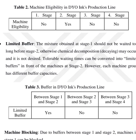
Stage 1, stage 3 and stage 4 have parallel identical machines on the other hand, there is machine eligibility restriction in stage 2 which has 4 machine groups related with job families. It refers that not all machines in this stage are capable of processing all jobs. It is due to dedication of subsets of machines for specific job families and each subset has parallel identical machines. A job coming from stage-1 is directed to the predetermined subset of machines depending on the family of job.
Table 2. Machine Eligibility in DYO Ink's Production Line 1. Stage 2. Stage 3. Stage 4. Stage
Machine
Eligibility No Yes No No
Limited Buffer: The mixture obtained at stage-1 should not be waited too long before stage-2, otherwise chemical decomposition (decaying) may occur, and it is not desired. Tolerable waiting times can be converted into “limited buffers” in front of the machines at Stage-2. However, each machine group has different buffer capacities.
Table 3. Buffer in DYO Ink's Production Line
Between Stage 1 and Stage 2 Between Stage 2 and Stage 3 Between Stage 3 and Stage 4 Limited Buffer Yes No No
Machine Blocking: Due to buffers between stage 1 and stage 2, machines in stage 1 can be blocked.
Table 4. Machine Blocking in DYO Ink's Production Line
Stage 1 Stage 2 Stage 3 Stage 4
Machine
Blocking Yes No No No
15 𝐹𝐻4 𝑨 ( 𝑃3(1), [𝑃1 (1), 𝑃3(2), 𝑃2(3), 𝑃2(4)] (2) , 𝑃3(3), 𝑃2(4) 𝑩 | 𝑆𝑠𝑑(1), 𝑏𝑙𝑜𝑐𝑘(1), 𝑏𝑢𝑓𝑓𝑒𝑟, 𝑀𝑘(2), 𝑆𝑠𝑑(3) 𝑪 | 𝐶𝑚𝑎𝑥 𝑫 )
A: To state Hybrid Flow Shop Scheduling with 4 stages
B: To represent machine types and machine numbers for each stage
Part C: To indicate Job Characteristics of the System17
CHAPTER THREE
LITERATURE SURVEY
Hybrid flow shop scheduling problem is encountered in many real world applications in different forms. Due to its relevance it has been studied extensively and hence has a wide range of literature.
First research about hybrid flow shop was introduced by Salvador (1970). His paper led other researchers to study on HFS problem. Garey and Johnson (1979) shown that the HFS problem with makespan minimization is NP-complete. The NP- nature of HFS problem has been studied along the years. In 1988, Gupta showed that the 2-stages HFS scheduling problem for makespan minimization NP- hard even if one stage has only one machine.
Many heuristics and approximation algorithms have been proposed for different variations of HFS depending on the machine configurations, job characteristics and objectives.
Ruiz and Vazguez- Rodriguez (2010) provided a comprehensive literature overview of HFS scheduling problem. They categorized studies depending on model structures and solution approaches. Their study provides the basis for our literature review. The list of studies included in their work has been extended by adding all relevant studies published after their work. However, some older papers (published before 1997) have not been taken into our list. Thus a list of 99 papers has been obtained. Their categorization has also been extended to obtain further information on modelling structures of the studies included in the list.
Two categorization tables have been prepared and presented in Appendix 1 and Appendix 2. The first table concerns with the modeling structures including the detail such as machine environments, job characteristics and objectives. In other words, this table shows which variant of HFS problem is considered in the respective study. If that table is reviewed, it can be seen that the studies mostly consider parallel identical machines in machine environments. The distribution of machine environments is shown in Figure 10.
18
Figure 10. Distribution of Machine Types in Literature
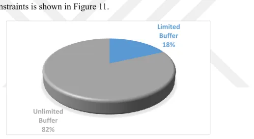
If buffer limitation is considered, most of studies concerns with unlimited buffer condition. It is assumed that it is due to complications arose with limited buffers. Even if limited buffers are studied, it is usually assumed that buffer size is 0. The distribution of buffer constraints is shown in Figure 11.
Figure 11. Distribution of Buffer Size in Literature
When setup times are considered, there are three categories which are “no setup times”, “sequence dependent setup times”, and “machine dependent setup times”. Researchers studied “no setup times” situation more than the others. The distribution of categories is shown in Figure 12. Identical Machines 79% Uniform Machines 7% Unrelated Machines 14% Limited Buffer 18% Unlimited Buffer 82%
19
Figure 12. Distribution of Setup Time in Literature
There may be many different performance measures for hybrid flow shop scheduling problem. However, an overwhelming majority of studies considers the objective of “minimizing makespan”. Distribution of performance measures is shown in Figure 13.
Figure 13. Distribution of Performance Measures in Literature
There are other constraints such as machines eligibility, preemption and precedence. There are few researches consider these constraints.
On the other hand, the table in Appendix-2 is related to solution methods, which are grouped as mathematical models, exact algorithms, heuristics and meta-heuristics. Distribution of solution approaches is shown in Figure 14.
No Setup Time 71% Sequence Dependent Setup 19%
Machine Dependent Setup 10% Makespan minimization 58% Several Objectives 20% Others 22%
20
Figure 14. Distribution of Solution Methodology in Literature
If a study is attributed to “mathematical model” with respect to solution methodology, then its model structure has been further investigated. Table 5 shows the properties of those studies.
Table 5. Properties of Mathematical Models in Literature
Paper Year Model Structure Solution Approach
Liu et al 2000
Basic Model + Sequence-dependent setup times (Minimizing tardiness, work in process and setup cost)
Lagrangian relaxation Liu et al 2008 Basic Model + Batch Process, no
buffers
Sawik 2000 Basic Model + Limited Buffer
(Blocking Scheduling)
Sawik 2001 Basic Model + Limited Buffer
(Blocking Scheduling)
Sawik et al 2002 Basic Model + Limited Buffer
(Blocking Scheduling)
Sawik 2002 Basic Model + Limited Buffer (Batch
Scheduling)
Sawik 2005
Basic Model + Batch Process and Limited Buffer (Minimizing Tardy Jobs)
Tang et al 2006
Basic Model + Limited Buffer (Total weighted completion time
minimization))
Lagrangian relaxation Tang et al 2006 Basic Model (Total weighted
completion time minimization)) Lagrangian relaxation
Tavakkoli-Moghaddam et al 2007
Basic Model + Sequence-dependent
setup times and Machine Blocking
Xuan et al 2007
Basic Model + Sequence-independent setup times and Batch production (the weighted completion time and the penalty of job waiting
minimization) Lagrangian relaxation 0 10 20 30 40 50
21
If a study is attributed to “meta-heuristics” with respect to solution methodologies, then it is required to identify which particular heuristics is meant such as Simulated Annealing (SA), Tabu Search (TS), Genetic Algorithms (GA), and Neural Networks (NN). The following figure shows the distribution of particular meta-heuristics utilized in the studies.
Figure 15. Distribution of Solution Methodologies in Literature
It is obvious that genetic and evolutionary algorithms take the greatest share. Tabu search and simulated annealing methods are the individual meta heuristic methods which follow genetic algorithm respectively. On the other hand, hybrid heuristics also take a considerable share. Neural network is the least preferred method among others.
Tabu Search 20%
Simulated Annealing
13%
Genetic & Evolutionary Algorithm 35% Hybrid 30% Neural Networks 2%
23
CHAPTER FOUR
MATHEMATICAL MODEL
In literature, although it may be found many studies that concern with the HFS problem, there are only a few papers involve in developing a detailed mathematical model since it is shown that even “basic” HFS problem is proven to be NP-hard in Gupta (1988). Gupta defined a “basic” HFS problem and formulated a MIP model. The basic model includes the following properties:
Manufacturing processes is divided into “m” stages or blocks in series. Each job has to be processed first at stage 1, then at stage 2, and so on. Each stage has a number of identical machines in parallel
Machine eligibility is not considered. Setup time is ignored.
Buffer is unlimited.
Machine Blocking is not considered. The objective is minimizing makespan.
One of the studies which discusses the mathematical formulation of the basic model was presented by Wang et al (2003). Kurz and Askin (2004) improved the mathematical model to include sequence-dependent setup times. Furthermore, Tavakkoli et al (2007) extended their model by inserting “machine blocking” constraints. A detailed breakdown of their model, assumptions, input parameters, indices, decision variables, and mathematical formulation as follows:
o Machines are available at all times, with no breakdowns or scheduled or unscheduled maintenance.
o Job processing cannot be interrupted.
o There is no buffer between stages, and processors can be blocked. o There is no travel time between stages.
24
o Machines in parallel are identical in capability and processing rate.
o Non-anticipatory sequence-dependent setup times exist between jobs at each stage. After completing processing of one job and before beginning processing of the next job, some sort of setup must be performed.
Input Parameters
m = number of processing stage. K = number of jobs.
ni = number of parallel processors in stage i. pik = processing time for job k in stage i.
silk = processor setup time for job k if job l is the immediately preceding job on the
processor i. Indices
i = processing stage, where i =1,…, m. j = processor in stage, where j =1,…, ni. k, l = job, where k, l =1,…, K.
Decision Variables
Cmax = makespan.
cik = completion time of job k at stage i. dik = departure time of job k from stage i.
xijlk = 1, if job k is assigned to processor j in stage i where job l is its predecessor job;
otherwise xijlk = 0. Two nominal jobs 0 and K+1 are considered as the first and
last jobs, respectively (Kurz and Askin, 2004). It is assumed that nominal jobs 0 and K+1 have zero setup and process time and must be processed on each processor in each stage.
Mathematical Formulation
𝑀𝑖𝑛 𝐶𝑚𝑎𝑥 Subject to
25 ∑ ∑𝐾𝑙=0,𝑙≠𝑘𝑥𝑖𝑗𝑙𝑘 𝑛𝑖 𝑗=1 = 1 ∀𝑖, 𝑘 (1) ∑𝐾𝑙=0,𝑙≠𝑘𝑥𝑖𝑗𝑙𝑘 = ∑𝐾+1𝑞=1,𝑞≠𝑘𝑥𝑖𝑗𝑘𝑞 ∀𝑖, 𝑗, 𝑘 (2) 𝑐1𝑘 ≥ 𝑝1𝑘+ ∑𝑛𝑖 𝑥1𝑗0𝑘𝑆𝑖0𝑘 𝑗=1 ∀𝑘 (3) 𝑐𝑖𝑘− 𝑐(𝑖−1)𝑘 ≥ 𝑝𝑖𝑘+ ∑𝑛𝑖 ∑𝐾𝑙=0𝑥𝑖𝑗𝑙𝑘𝑆𝑖𝑙𝑘 𝑗=1 ∀𝑖 > 1, 𝑘 (4) 𝑐𝑖𝑘 ≥ 𝑝𝑖𝑘 + ∑ ∑𝐾𝑙=0,𝑙≠𝑘𝑥𝑖𝑗𝑙𝑘(𝑆𝑖𝑙𝑘+ 𝑑𝑖𝑙) 𝑛𝑖 𝑗=1 ∀𝑖, 𝑘 = 1, … , 𝐾 + 1 (5) 𝑐𝑖𝑘 = 𝑑(𝑖−1)𝑘+ 𝑝𝑖𝑘+ ∑ ∑𝐾𝑙=0𝑥𝑖𝑗𝑙𝑘𝑆𝑖𝑙𝑘 𝑛𝑖 𝑗=1 ∀𝑖 > 1, 𝑘 (6) 𝑐𝑚𝑘 = 𝑑𝑚𝑘 ∀𝑘 (7) 𝐶𝑚𝑎𝑥 ≥ 𝑐𝑚𝑘 ∀𝑘 (8) 𝑥𝑖𝑗𝑙𝑘 ∈ {0,1} ∀𝑖, 𝑗, 𝑙, 𝑘 (9) 𝑐𝑖𝑘, 𝑑𝑖𝑘 ≥ 0 ∀𝑖, 𝑘 (10)
The objective is to minimize the makespan. Constraint-1 ensures that each job k in every stage is assigned to only one processor immediately after job l. Constraint-2 is complementary to constraint 1. It is a flow balance constraint and it determines which processors at each stage must be scheduled. Constraint-3 calculates the complete time for the first available job on each processor at stage-1. Likewise, Constraint-4 calculates the completion time for the first available job on each processor in other stages, and also guarantees that each job is processed in all downstream stages with regard to setup time related to both the job to be processed and the immediately preceding job. Constraint-5 controls the machine blocking. Constraint-6 calculates the processing of a job depending on the processing of its predecessor on the same processor in a given stage. This constraint controls creating the processor's idle time. Both constraint sets 5 and 6 ensure that a job cannot begin setup until it is available and the previous job at the current stage is complete. Constraint-6 indicates that the processing of each job in every stage starts immediately after its departure from the previous stage and plus the setup time of the immediately preceding job. Constraint-7 ensures that each product leaves the system when it is completed in the latest stage. Constraint-8 defines the maximum completion time.
26
In our case study, operational characteristics of HFS problem implies that it includes limited buffers and machine eligibility restrictions in addition to machine blocking and sequence-dependent setup times. To the best of our knowledge, there is no formulation in literature which considers all those operational characteristics (constraints) together. Therefore, an original mathematical model is proposed to represent true properties of our real HFS problem. The model has the following assumptions.
1. Machines are available at all times. There are no breakdowns or maintenance. 2. Job processing cannot be interrupted (i.e., no preemption is allowed) and jobs have no associated priority values.
3. There are limited buffers between stage1 and stage 2. Therefore, machines in stage 1 may be blocked if all machines are busy at stage 2 when jobs are finished at stage 1.
4. There is no travel time between stages; jobs are available for processing at a stage immediately after departing at previous stage.
5. The ready time for all jobs is zero.
6. Machines in parallel are identical at stage 1, stage 3 and stage 4 in capability and processing rate.
7. There are machine groups at stage 2 and these groups have parallel machines which are identical in capability and processing rate. Machine groups are defined since certain jobs can be processed only on certain machines or only a predetermined subset of machines. This requirement imposes “machine eligibility” constraints.
8. Sequence-dependent setup times exist between jobs at stage 1 and stage 3. Development of proposed model will be presented in phases. In the first phase, all job characteristics are ignored and a standard (basic) model is defined. In the following phases, job characteristics will be inserted one by one to represent more realistic environments.
Basic Hybrid Flow Shop Model (M0)
The details of input parameters, indices, decision variables and mathematical formulation of the basic model are presented below.
27
M = number of stages. K = number of jobs.
ni = number of parallel machines in stage i. pik = processing times for job k in stage i. Q = a large number.
Indices
i =processing stage, where i =1,...,M.
j =machine in stage, where j =1,…, ni.
k, l =jobs, where k, l =1,...,K.
Decision Variables
Cmax = makespan.
stik = starting time of job k at stage i.
xijk= { 0, otherwise 1, if job k is assigned to machine j in stage i
yijkl= {
1, if job k precedes job l on machine j at stage i 0, otherwise Mathematical Formulation 𝑀𝑖𝑛 𝐶𝑚𝑎𝑥 Subject to 𝐶𝑚𝑎𝑥 ≥ 𝑠𝑡𝑖𝑘+ 𝑝𝑖𝑘 ∀𝑖, 𝑘 (1) 𝑦𝑖𝑗𝑘𝑙≤ 𝑥𝑖𝑗𝑘 ∀𝑖, 𝑗, 𝑘, 𝑙 𝑖𝑓 𝑘 ≠ 𝑙 (2) 𝑦𝑖𝑗𝑘𝑙≤ 𝑥𝑖𝑗𝑙 ∀𝑖, 𝑗, 𝑘, 𝑙 𝑖𝑓 𝑘 ≠ 𝑙 (3) 1 + ∑𝐾𝑘=1∑𝐾𝑙=1,𝑙≠𝑘𝑦𝑖𝑗𝑘𝑙 = ∑𝐾𝑘=1𝑥𝑖𝑗𝑘 ∀𝑖, 𝑗 (4) ∑𝑛𝑖 𝑦𝑖𝑗𝑘𝑙 𝑗=1 + ∑𝑛𝑗=1𝑖 𝑦𝑖𝑗𝑙𝑘 ≤ 1 ∀𝑖, 𝑘, 𝑙 𝑖𝑓 𝑘 ≠ 𝑙 (5) ∑𝐾𝑙=1,𝑙≠𝑘𝑦𝑖𝑗𝑘𝑙 ≤ 1 ∀𝑖, 𝑗, 𝑘 (6)
28 ∑𝐾𝑘=1,𝑘≠𝑙𝑦𝑖𝑗𝑘𝑙 ≤ 1 ∀𝑖, 𝑗, 𝑙 (7) ∑𝑛𝑗=1𝑖 𝑥𝑖𝑗𝑘 = 1 ∀𝑖, 𝑘 (8) ∑𝐾𝑘=1𝑥𝑖𝑗𝑘 ≥ 1 ∀𝑖, 𝑗 such that 𝐾 ≥ 𝑛𝑖 (9) ∑ ∑𝑛𝑖 𝑗 𝑥𝑖𝑗𝑘 𝑗=1 ≥ 𝐾(𝐾+1) 2 𝐾 𝑘=1 ∀𝑖 such that 𝐾 < 𝑛𝑖 (10) 𝑄(1 − ∑𝑛𝑗=1𝑖 𝑦𝑖𝑗𝑘𝑙) + 𝑠𝑡𝑖𝑙 ≥ 𝑠𝑡𝑖𝑘+ 𝑝𝑖𝑘 ∀𝑖, 𝑘, 𝑙 𝑖𝑓 𝑘 ≠ 𝑙 (11) 𝑠𝑡(𝑖+1)𝑘 ≥ 𝑠𝑡𝑖𝑘 + 𝑝𝑖𝑘 ∀𝑖 < 𝑀, 𝑘, 𝑙 (12) 𝑠𝑡𝑖𝑘 ≥ 0 ∀𝑖, 𝑘 (13) 𝑥𝑖𝑗𝑘 ∈ {1,0} ∀𝑖, 𝑗, 𝑘 (14) 𝑦𝑖𝑗𝑘𝑙 ∈ {1,0} ∀𝑖, 𝑗, 𝑘, 𝑙 (15)
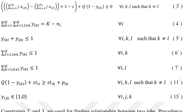
The objective is minimizing the completion time of last job (makespan). Constraint-1 finds the makespan. Constraints 2 and 3 are used for finding relationship between two jobs. It means if two jobs are assigned to same machine at any stage, these control that one of these jobs precedes the other. Precedence number is brought under control with constraint-4. Constraint-5 is also related to precedence and it provides that two jobs cannot precede each other. Constraints 6 and 7 are complementary to constraint 5. These make sure that one job can precede only one job and one job can be preceded by only one job. Constraint-8 guarantees all operations are assigned only one machine in each stage. Usage of each machine in each stage is controlled by constraints 9 and 10. One of these constraints is used according to job numbers and machine numbers. Constraints 11 and 12 control start times of each job in each stage. Constraint-11 provides that any job can be started at a stage if preceding job completes the process. Constraint-12 ensures that each job can be started at a stage if it has been completed at previous stage.
The number of decision variables and the number of constraints for this model (M0) can be expressed in terms of input parameters. Let N be total number of machines in the overall system, where
29 𝑁 = ∑ 𝑛𝑖
𝑀
𝑖=1
Table 6. Number of Decision Variables in Model (M0)
Source Number Of Variables Binary xijk and yijkl (𝐾2𝑁 + 𝐾𝑁)
Real stik and Cmax (𝐾𝑀 + 1)
Number of Constraints = (3𝐾𝑀) + 2𝑁 + 2[𝐾(𝐾 − 1)𝑁] + 2[(𝐾 − 1)𝑁] +[𝐾(𝑀 − 1)] + 3 [𝐾(𝐾−1)𝑀 2 ] = (3𝐾𝑀) + [(2𝑁(1 + 𝐾2− 𝐾 + 𝐾 − 1)] + [𝐾 ((2𝑀)−2+(3𝐾𝑀)−(3𝑀 2 )] = (3𝐾𝑀) + (2𝐾2𝑁) + [𝐾 ((3𝐾𝑀)−𝑀−2) 2 )] = 𝐾 [(5𝑀) + (4𝐾𝑁) + (3𝐾𝑀) − 2 2 ]
For example, consider a HFS problem such that there are four stages. Stages 1 &2 both have 2 identical machines in parallel. Stage-3 has one machine whereas Stage-4 has 3 identical machines in parallel. Assume that there are 100 jobs. This problem would have 80.800 binary variables, 401real variables and 220.900 constraints.
The basic model above is reviewed whether it is possible to reduce the number of decision variables and number of constraints. It has been shown that a modified model (MM0) can be formulated using a different perspective. Modified model is based on the basic one, however the following changes have been made.
ε = a small number
yikl= {
1, if job k precedes job l at stage i 0, otherwise
Notice that decision variable y has now 3 indices instead of 4 as in previous basic model. (((∑ 𝑗 𝑥𝑖𝑗𝑘 𝑛𝑖 𝑗=1 ) − (∑ 𝑗 𝑥𝑖𝑗𝑙 𝑛𝑖 𝑗=1 )) − 1 + 𝜀) − 𝑄 (1 − 𝑦𝑖𝑘𝑙) ≤ 0 ∀𝑖, 𝑘, 𝑙 such that 𝑘 ≠ 𝑙 ( 2’ )
30 (((∑ 𝑗 𝑥𝑖𝑗𝑘 𝑛𝑖 𝑗=1 ) − (∑ 𝑗 𝑥𝑖𝑗𝑙 𝑛𝑖 𝑗=1 )) + 1 − 𝜀) + 𝑄 (1 − 𝑦𝑖𝑘𝑙) ≥ 0 ∀𝑖, 𝑘, 𝑙 such that 𝑘 ≠ 𝑙 ( 3’ ) ∑𝐾𝑘=1∑𝐾𝑙=1,𝑙≠𝑘𝑦𝑖𝑘𝑙 = 𝐾 − 𝑛𝑖 ∀𝑖 ( 4’ ) 𝑦𝑖𝑘𝑙+ 𝑦𝑖𝑙𝑘 ≤ 1 ∀𝑖, 𝑘, 𝑙 such that 𝑘 ≠ 𝑙 ( 5’ ) ∑𝐾𝑙=1,𝑙≠𝑘𝑦𝑖𝑘𝑙 ≤ 1 ∀𝑖, 𝑘 ( 6’ ) ∑𝐾𝑘=1,𝑘≠𝑙𝑦𝑖𝑘𝑙 ≤ 1 ∀𝑖, 𝑙 ( 7’ ) 𝑄(1 − 𝑦𝑖𝑘𝑙) + 𝑠𝑡𝑖𝑙 ≥ 𝑠𝑡𝑖𝑘 + 𝑝𝑖𝑘 ∀𝑖, 𝑘, 𝑙 such that 𝑘 ≠ 𝑙 ( 11’ ) 𝑦𝑖𝑗𝑘 ∈ {1,0} ∀𝑖, 𝑗, 𝑘 ( 15’ )
Constraints 2’ and 3’ are used for finding relationship between two jobs. Precedence
number is brought under control with constraint-4’. Constraint-5’ provides that two
jobs cannot precede each other. Constraints 6’ and 7’ are complementary to constraint
5 and these ensure one job can precede only one job and one job can be preceded by only one job. Constraint-11’ controls start times of each job in each stage. It means any
job can be started at a stage if preceding job completes the process.
The number of decision variables and the number of constraints for modified basic model (MM0) can be found as follows.
Table 7. Number of Decision Variables in Modified Model (MM0)
Source Number Of Variables Binary xijk and yijkl (𝐾2𝑀) + 𝑁
Real stik and Cmax (𝐾𝑀) + 1
Number of Constraints = (3𝐾𝑀) + 11 (𝐾(𝐾−1)𝑀 2 ) + [𝐾(𝑀 − 1)] + 𝑀 + 𝑁 = (6𝐾𝑀)+(11𝐾2𝑀)−(11𝐾𝑀)+(2𝑀)+(2𝑁)+(2𝐾𝑀)−(2𝐾) 2 =(11𝐾 2𝑀) − (3𝐾𝑀) + 2(𝑀 + 𝑁 − 𝐾) 2
31
If the same previous example is considered, the problem would have 40.008 binary variables, 401 real variables and 219.312 constraints.
Table 8. Comparison of Structure of Basic Model and Modified Basic Model
Number of Decision Variables Number of Constraints
Binary Real
Basic Model (M0) 80.800 401 220.900
Modified Basic Model (MM0) 40.008 401 219.312 It is clear that the number of variables in modified basic model are much less than those of basic model. It leads to the expectation that the solution time in modified basic model would be decreased. In order to test this assumption, a sample problem has been designed. Sample problem involves 3 stages having 3, 2 and 4 identical machines in parallel respectively. Processing times are chosen randomly. Sample problem has been solved using both models and it is seen that the solution time is decreased considerably. The outcomes are summarized in the following table.
Table 9. Performance Comparison of Basic and Modified Basic Models
Solution ( Cmax) Solution Time (seconds)
Basic Model (M0) 33 82.12
Modified Basic Model (MM0) 33 8.53
Henceforth we will use the modified basic model (MM0) in order to construct extended models by inserting additional constraints that represent more realistic environments.
Hybrid Flow Shop Model With Machine Blocking (M1)
When a job on a machine in any stage completes its operation, it moves to next stage for the next operation but all the machines at the next stage may be busy and hence unavailable at that time. In that case, the job is put in a queue in front of the next stage. However, there may be no space for a job queue (no buffer). Even if there is a space to allow a job queue, it is usually limited (limited buffer). If two successive stages have no buffer in between or if there is a limited buffer and the job queue is full, then the job does not move to next stage and it remains on and block the machine until a downstream machine or queue becomes available. It is called machine blocking. In order to include machine blocking situation in our model, a new constraint is inserted as follows:
32 𝑀𝑖𝑛 𝐶𝑚𝑎𝑥
Subject to
MM0 constraints (1) – (15)
𝑄 (1 − 𝑦𝑖𝑘𝑙) + 𝑠𝑡𝑖𝑙 ≥ 𝑠𝑡(𝑖+1)𝑘 ∀𝑖 < 𝑀 ∀𝑘, 𝑙 such that 𝑘 ≠ 𝑙 (16)
Constraint-16 work with constraints 11 and 12 in model (MM0) and it provides that any job can be started if precedence job in downstream machine completes process. Please note that machine blocking constraint works if there is no buffer between stages. If there is limited buffer, then the model has to be modified further. That situation is mentioned below in the model (M3).
Hybrid Flow Shop Model With Machine Blocking And Sequence Dependent Setup Times (M2)
Setup time is divided by two parts which are sequence dependent setup times, and machine dependent setup times. Sequence-dependent times depends on both the current and preceding job, and machine-dependent times depends on the current job to be processed. In our study only sequence dependent setup times are considered. In order to incorporate setup times, the model is modified as follows.
New Input Parameter
sikl = setup time for job l if job k is the immediately preceding job in sequence
operation on the stage i. 𝑀𝑖𝑛 𝐶𝑚𝑎𝑥
Subject to
Model (M1) constraints (1) – (10) and (13) – (15)
𝑄 (1 − 𝑦𝑖𝑘𝑙) + 𝑠𝑡𝑖𝑙 ≥ 𝑠𝑡𝑖𝑘 + 𝑝𝑖𝑘+ 𝑠𝑖𝑘𝑙 𝑦𝑖𝑘𝑙 ∀𝑖, 𝑘, 𝑙 𝑠𝑢𝑐ℎ 𝑡ℎ𝑎𝑡 𝑘 ≠ 𝑙 (11’’)
𝑠𝑡(𝑖+1)𝑘 ≥ 𝑠𝑡𝑖𝑘 + 𝑝𝑖𝑘+ 𝑠(𝑖+1)𝑙𝑘 𝑦(𝑖+1)𝑙𝑘 ∀𝑖 < 𝑀 ∀𝑘, 𝑙 𝑠𝑢𝑐ℎ 𝑡ℎ𝑎𝑡 𝑘 ≠ 𝑙 (12’) 𝑄 (1 − 𝑦𝑖𝑘𝑙) + 𝑠𝑡𝑖𝑙 ≥ 𝑠𝑡(𝑖+1)𝑘+ 𝑠𝑖𝑘𝑙 𝑦𝑖𝑘𝑙 ∀𝑖 < 𝑀 ∀𝑘, 𝑙 𝑠𝑢𝑐ℎ 𝑡ℎ𝑎𝑡 𝑘 ≠ 𝑙 (16’)
33
Setup time part is included in constraints 11’, 12, and 16 in M1. As it is explained
before, these constraints control start times of each job at each stage.
Hybrid Flow Shop Model With Machine Blocking, Sequence Dependent Setup Times And Limited Buffer (M3)
In this phase, “limited buffer” constraint will be inserted into the model. Please remember that the model (M2) above assumes that there is no buffer between stages. This assumption is inherited from model (M1). Sawik (2000) proposed an idea to surpass the difficulty and hence insert a “limited buffer” constraint. The idea is simple: add a dummy stage in between two true successive stages. Dummy stage has dummy machines with zero processing times. The number of dummy machines is equal to the size of buffer. In that case, you may still assume no buffer between stages, however dummy stage imitates “limited buffer”. Sawik’s idea may be incorporated in our model as follows.
New Input Parameters
B = number of stages that have limited buffers bq= index for artificial stage corresponds to buffers
New Indices
i = processing stage, where i =1,...,(M+B) q = buffer, where q=1,...,B
𝑀𝑖𝑛 𝐶𝑚𝑎𝑥
Subject to
M2 constraints (1) – (11) and (13) – (15)
𝑠𝑡(𝑖+1)𝑘 ≥ 𝑠𝑡𝑖𝑘+ 𝑝𝑖𝑘+ 𝑠(𝑖+1)𝑙𝑘 𝑦(𝑖+1)𝑙𝑘 ∀𝑖 < 𝑀 + 𝐵, 𝑘, 𝑙 (12’’)
𝑄(1 − 𝑦𝑖𝑘𝑙) + 𝑠𝑡𝑖𝑙≥ 𝑠𝑡(𝑖+1)𝑘+ 𝑠𝑖𝑘𝑙𝑦𝑖𝑘𝑙 ∀𝑖 < 𝑀 + 𝐵 ∀𝑘, 𝑙 such that 𝑘 ≠ 𝑙 and (16’’)
(𝑏𝑞− 1) ≤ 𝑖 ≤ 𝑏𝑞 ∀𝑞
Buffer stages are included in limits of 12’’ and 16’’. In addition, execution area of
34
Hybrid Flow Shop Model With Machine Blocking, Sequence Dependent Setup Times, Limited Buffers And Machine Eligibility (M4)
In a hybrid flow shop line, sometimes a job may not be processed on some of the machines at a stage because of some technical or technological limitations. In other words, parallel machines at a stage may not be capable of processing all jobs. This requirement (constraint) is defined as “machine eligibility”. In our case study, there are family groups (job types) and jobs can be processed only on the machines which are dedicated to the corresponding family groups. This rule applies only at Stage-2. In that stage, parallel machines are grouped depending on the family groups (job types). Machine eligibility constraint is inserted in our model as follows.
New Input Parameters
G = number job types
Si = set of machine in stage i
Fig = set of machines for job type g in stage i, Fig∈ Si
fk = job type of job k
New Indices
g =job types, where g =1,...,G
𝑀𝑖𝑛 𝐶𝑚𝑎𝑥
Subject to
M3 constraints (1) – (16)
∑𝑗∈𝐹𝑖𝑔𝑥𝑖𝑗𝑘 = 1 ∀𝑖, 𝑗, 𝑘, 𝑔 such that 𝑓𝑘 = 𝑔 (17)
Constraint-17 guarantees that all jobs are assigned to machines according job types and machine groups at each stage.