Comparing the performance of humans and 3D-convolutional neural networks in material perception using dynamic cues

(1)

COMPARING THE PERFORMANCE OF

HUMANS AND 3D-CONVOLUTIONAL

NEURAL NETWORKS IN MATERIAL

PERCEPTION USING DYNAMIC CUES

a thesis submitted to

the graduate school of engineering and science

of bilkent university

in partial fulfillment of the requirements for

the degree of

master of science

in

neuroscience

By

Hossein Mehrzadfar

July 2019

(2)

Comparing the Performance of Humans and 3D-Convolutional Neural Networks in Material Perception Using Dynamic Cues

By Hossein Mehrzadfar July 2019

We certify that we have read this thesis and that in our opinion it is fully adequate, in scope and in quality, as a thesis for the degree of Master of Science.

H¨useyin Boyacı(Advisor)

Tolga C¸ ukur

Selen Pehlivan

Approved for the Graduate School of Engineering and Science:

Ezhan Kara¸san

(3)

ABSTRACT

COMPARING THE PERFORMANCE OF HUMANS

AND 3D-CONVOLUTIONAL NEURAL NETWORKS IN

MATERIAL PERCEPTION USING DYNAMIC CUES

Hossein Mehrzadfar M.S. in Neuroscience Advisor: H¨useyin Boyacı

July 2019

There are numerous studies on material perception in humans. Similarly, there are various deep neural network models that are trained to perform different visual tasks such as object recognition. However, the intersection of material perception in humans and deep neural network models has not been investigated to our knowledge. Especially, the importance of the ability of deep neural net-works in categorizing materials and also comparing human performance with the performance of deep convolutional neural networks has not been appreci-ated enough. Here we have built, trained and tested a 3D-convolutional neural network model that is able to categorize the animations of simulated materials. We have compared the performance of the deep neural network with that of hu-mans and concluded that the conventional training of deep neural networks is not necessarily giving the optimal state of the network to be compared to the perfor-mance of the humans. In the material categorization task, the similarity between the performance of humans and deep neural networks increases and reaches the maximum similarity and then decreases as we train the network further. Also, by training the 3D-CNN on regular, temporally consistent animations and also training it on the temporally inconsistent animations and comparing the results we found out that the 3D-CNN model can use spatial information in order to cat-egorize the material animations. In other words, we found out that the temporal, and consistent motion information is not necessary for the deep neural networks in order to categorize the material animations.

Keywords: Deep Neural Networks, 3D-Convolutional Neural Networks, Material Perception, Material Animations, Motion Perception.

(4)

¨

OZET

˙INSANLARIN PERFORMANSINI KARS¸ILAS¸TIRMAK

VE 3D-KONVOLEKS˙IYONEL N ¨

ORAL A ˘

GLARDA

D˙INAM˙IK P˙IS

¸ ˙IRME KULLANILAN MALZEME

ANLAYIS

¸I

Hossein Mehrzadfar Nörobilim, Yüksek Lisans Tez Danı¸smanı: Hüseyin Boyacı

July 2019

˙Insanlarda materyal algısı üzerine ¸cok sayıda ¸calı¸sma var. Benzer ¸sekilde, nesne tanıma gibi farklı görsel görevleri yerine getirmek üzere e˘gitilmi¸s ¸ce¸sitli derin sinir a˘gı modelleri de vardır. Bununla birlikte, insanlarda materyal algısinın kesi¸sti˘gi ve derin sinir a˘gı modellerinin bilgisine bakılmamı¸stır. Ozellikle, de-¨ rin sinir a˘glarının malzemelerin sınıflandırılmasındaki, ve insan performansını de-rin evri¸simli sinir a˘glarının performansıyla kar¸sıla¸stırabilmesinin önemi yeterince anla¸sılmamı¸stır. Burada, simüle edilmi¸s malzemelerin animasyonlarını katego-rize edebilen 3 boyutlu evri¸simsel sinir a˘gı modelini kurduk, e˘gitdik ve test ettik. Derin sinir a˘gının performansını insanlarla kar¸sıla¸stırdık, ve derin sinir a˘glarının konvansiyonel e˘gitiminin insan a˘gının performansıyla kar¸sıla¸stırılması i¸cin en uy-gun a˘g durumu vermek zorunda olmadı˘gına karar verdik. Materyal sınıflandırma görevinde, insanların performansı ile derin sinir a˘glarının performansı arasındaki benzerlik maksimum seviyeye ulasana kadar artar, azami benzerli˘ge ula¸sır ve daha sonra a˘gı e˘gittik¸ce azalır. Ayrıca, 3D-CNN’i düzenli ve ge¸cici olarak tutarlı animasyonlar üzerinde e˘giterek ve ge¸cici olarak tutarsız animasyonlar üzerinde e˘giterek ve bu sonu¸cları kar¸sıla¸stırarak 3D-CNN modelinin malzeme animasyon-larını kategorize etmek i¸cin mekansal bilgileri kullanabilece˘gini gördük. Ba¸ska bir deyi¸sle, derin sinir a˘gları i¸cin zamansal ve tutarlı hareket bilgilerinin materyal animasyonları sınıflandırmak i¸cin gerekli olmadı˘gını ö˘grendik.

Anahtar sözcükler : Derin Sinir A˘gları, Ü¸c Boyutlu Evri¸simsel Sinir A˘gları, Malzeme Algısı, Malzeme Animasyonları, Hareket Algısı.

(5)

Acknowledgement

First, I want to thank my father and mother for their encouragement and support, making them happy truly is and always was one of the biggest goals in my life. I want to thank my family, Mohammad, Zohreh, Ali, Fatemeh, Ahmad, and my dearests Niousha & Armin, for their unconditional love and support, without them this was not possible.

I would like to thank my advisers Prof. Huseyin Boyaci and Prof. Katja Doerschner for their patience and support throughout my master’s degree. They are easily the best and nicest academic advisers that I have ever met. Their excellence in research and enthusiasm for guiding me as a graduate student helped me a lot and encouraged me to chose to be an academic researcher in the future. So, thank you for everything!

I would like to thank my teachers, Dr. Borchlou, Dr. Inanlou, Dr. Bahrami, Dr. Yoonessi, Dr. Hulusi Kafalıgonul, Dr. Tolga Ç ukur, Dr. Michelle Adams, and Dr. Burcu Ay¸sen Ürgen for helping me on this journey. I like to thank Dr. Alexandra Schmid and Ms. Buse Merve Ürgen who were my unofficial teachers and helped me a lot. Also, I want to thank Dr. Ergin Atalar, the director of UMRAM and Ms. Aydan Ercingoz, administrative assistant of UMRAM and all of the staff in UMRAM for providing an excellent and world-class environment to study the brain!

Finally, I would like to thank my friends and labmates, Mina Elhamiasl, Gorkem Er, Timucin Bas, Cem Benar, Hamidreza Farhat, Behnam Darzi, Hamed Azad, Cemre Yılmaz, Ali Yousefimehr, Ecem Altan, Batuhan Erkat, ˙Ilayda Nazlı, Dilara Eri¸sen, Beyza Akkoyunlu, Shahram, Reza Kiani, Reza Abbasi, Reza kashi, Mostafa, Milad, and Dada Rostam. Thank you all for your companionship and positive energy.

(6)

List of Figures

1.1 Single Perceptron[1]. Inputs x1, x2, ..., xn are multiplied with the weights w1, w2, ..., wnand summed up with bias b and then the ϕ(·) function is applied in order to create the output y. . . 3

2.1 Eight consecutive frames of the animations for each action. . . 11

2.2 The behavioral test set-up in Experiment 1 and Experiment 2. The target stimuli was shown in the middle and the test animations were show in the surrounding spots. . . 14

3.1 The confusion matrix of the behavioral test. Dark red colour shows perfect correlation and dark blue shows zero correlation. . . 20

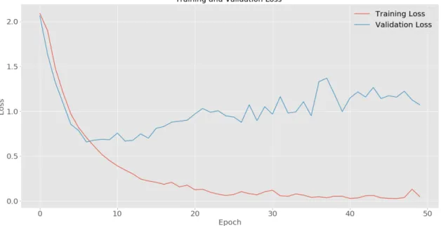
3.2 Training and validation loss for 50 epochs. . . 21

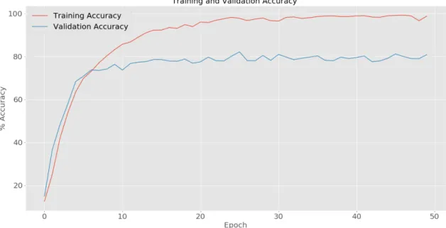
3.3 Training and validation accuracy for 50 epochs. . . 22

3.4 Confusion Matrix for the DNN model during training, the Epoch 0, Epoch 1, Epoch 5, Epoch 10, Epoch 15, Epoch 20. . . 24

3.5 Spearman Correlation for the temporally consistent animations . . 25

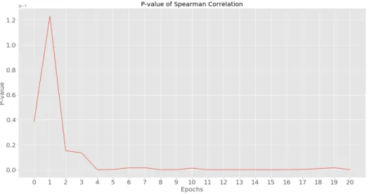
3.6 P-value of Spearman Correlation for the temporally consistent an-imations . . . 26

(9)

LIST OF FIGURES ix

3.7 Training and validation loss for 50 epochs when 3D-CNN model is trained using the temporally inconsistent animations. . . 28

3.8 Training and validation accuracy for 50 epochs when 3D-CNN model is trained using the temporally inconsistent animations. . . 29

3.9 Spearman Correlation when 3D-CNN model is trained using the temporally inconsistent animations. . . 30

3.10 P-value of Spearman Correlation when 3D-CNN model is trained using the temporally inconsistent animations. . . 31

3.11 Feature map of layer 1 after 3D-Convolution. 25 sample feature maps of the first layer are shown. Each feature map is 128 × 128 which is the size of the output of the first layer. In each feature map dark purple shows zero response of the respective filter and yellow shows the highest response. . . 33

3.12 The color code for the Fig 3.9 to Fig 3.21. According to this color code, dark purple shows zero response of the filter and yellow shows the highest response. . . 33

3.13 Feature map of layer 1 after 3D-MaxPooling. Here we can see that the dimension have become 64 × 64 which is the dimension of the output of the first layer after 3D-Max pooling. We can see that the filters are responsive to edges and corners of the object. . . 34

3.14 Feature map of layer 2 after 3D-Convolution. We can see that because of temporal convolution and max pooling in the time di-mension, feature maps are showing some sense of motion compared to previous layer. . . 35

(10)

LIST OF FIGURES x

3.15 Feature map of layer 2 after 3D-MaxPooling.Here because of the max pooling which shrinks the input in time domain, we cans see that feature maps are responsive to multiple frames and showing motion. . . 36

3.16 Feature map of layer 3 after 3D-Convolution. We can see that some filters are responsive to the whole object in this layer. . . 37

3.17 Feature map of layer 4 after 3D-Convolution. . . 38

3.18 Feature map of layer 4 after 3D-MaxPooling. Max pooling shrinks the data in spatial and temporal domains and in this layer infor-mation from multiple frames are extracted and therefore we cannot see the actual shape of the object anymore. . . 39

3.20 Feature map of layer 6 after 3D-Convolution. Here the feature map is activated sparsely and all temporal and spatial features of the animations are collapsed because of the convolutions and max poolings in the network. . . 41

3.21 Feature map of layer 6 after 3D-MaxPooling. . . 42

3.23 Feature map of layer 8 after 3D-Convolution. Here the feature map is sparsely activated, but this is useful because these few activa-tions are actually contributing to determine the final label of the animation. . . 44

3.24 t-SNE Visualization for the Output of the 3D Conv 1 Layer. . . . 45

3.25 t-SNE Visualization for the Output of the 3D MaxPool 1 Layer. . 46

(11)

LIST OF FIGURES xi

3.37 t-SNE Visualization for the Output of the Fully Connected 9 Layer. 58

(12)

List of Tables

2.1 Distribution of number of videos with specific actions per category. These videos were categorized by participants to 8 different cate-gories and for each category 1040 videos were selected randomly to be used as input data for the deep neural network model. . . . 12

2.2 Number of animations in each perceptual category. . . 14

2.3 DNN Architecture, shape of the tensors, and the number of pa-rameters for each layer. . . 18

3.1 Classification Report After 16 Epochs when 3D-CNN model is trained and tested using regular animations. . . 23

3.2 Classification Report After 16 Epochs when 3D-CNN model is trained using regular animations but tested using the temporally inconsistent animations. . . 27

3.3 Classification Report After 16 Epochs when 3D-CNN model is trained using the temporally inconsistent animations. . . 32

(13)

Chapter 1 Introduction

1.1 Purpose of The Study

In recent years various deep neural network models have been built to simulate some of the internal processes of the human brain or in order to simulate human behavior. Especially, human vision frequently has been compared to deep neu-ral networks. Here, we are using a special type of deep neuneu-ral networks called 3D-convolutional neural networks as a computational model for categorizing an-imations of objects with different material properties. The performance of deep neural networks in categorizing material animations will be compared with that of humans. By randomly shuffling the frames of these animations, the degree to which these deep neural networks are using temporal information in order to classify the animations will be determined.

(14)

1.2 Deep Neural Network Models

1.2.1 What is a Deep Neural Network?

In 1943 Warren McCulloch and Walter Pitts proposed the first mathematical model of the biological neurons which was a unit with inputs and one output. It was getting various inputs and based on the weighted sum of the inputs and comparing it to the threshold of the neuron the output was either 0 or 1 [2]. Based on this model, a psychologist named Frank Rosenblatt introduced the idea of the Perceptron, later in 1958 [3]. A perceptron is a unit that is inspired by bi-ological neurons and it has the ability to learn the patterns in the data, however, it could act as a simple linear classifier and it was not able to classify the data that were not linearly separable. One way to solve this problem was by putting these units of perceptrons together in layers and connecting the layers in a way that outputs of the perceptrons in earlier layers were the inputs for the percep-trons in the next layer. Scientists in that era, including Marvin Minsky, were skeptical about such an approach and thought that training such networks would take a very long time if not forever [4]. These skepticism discouraged many sci-entists to work on neural networks and shifted the flow of funds away from these studies and later led to an era called the first ”Artificial Intelligence (AI) Winter”.

Later in around 1990, the idea of neural networks was completely revitalized by the efforts of Werbos, Williams, Hinton, and Rumelhart and many others. Multi-Layer Perceptrons have an input layer, an output layer, and some hidden layers and this time they were proven to be functional using Backpropagation and Gradient Descent methods. Backpropagation is basically using the chain rule to calculate the derivatives of the errors that are made by the neural network and backpropagating it to previous layers and individual neurons in those layers [5]. In this way, it will be known that how much each individual neuron was respon-sible for pushing the neural network to reach a wrong conclusion (classifying the input in the wrong category). However, only knowing the amount of error and the contribution of each individual neuron to that is not enough to have a functioning

(15)

Figure 1.1: Single Perceptron[1]. Inputs x1, x2, ..., xn are multiplied with the weights w1, w2, ..., wn and summed up with bias b and then the ϕ(·) function is applied in order to create the output y.

(16)

neural network. Gradient Descent is an optimization technique that changes the weights between the neurons in order to push the network toward the minimum of the error/cost function. In this way, after each iteration, the network will do a slightly better job because after making a mistake (misclassification) the error will be backpropagated through the network and the weights and biases for each neuron will be modified in a way that it helps the whole network to reach better results and minimize the error..

1.2.2 The Convolutional Neural Networks

The convolutional neural networks are specific kind of neural networks that are specialized to extract the spatial information from images mainly. Instead of having individual weights for each neuron they have a grid of several neurons called filters. One can say that a convolutional neural network is a multilayer perceptron after removing many weights and connections and keeping some very special connections between the layers. These filters are swept across the input pixels of the image in both spatial dimensions. Row by row and column by column the value of the input pixels are convolved with the initialized weights of each neuron in the filters. The output of each filter go to the next layer and becomes the input for the next layer’s filters. Each filter ends up being more responsive to a specific feature. For example, in the early layers of a convolutional neural network, the filters are responsive to the line, edge, and corner patterns in the images and as we go deeper in the network by combining these features, filters extract more complex patterns like specific shapes.

The convolutional neural networks have been used extensively in object and face recognition [6, 7], object detection [8], image classification [9], and action recognition [10] in the academia and industry. Also, the research in comparing the convolutional neural networks with human brain and behavior is growing. For example, Cichy et.al.[6] have compared object recognition in the deep con-volutional neural networks and human brain and showed that layers of deep

(17)

convolutional neural networks correspond to the various visual processing stages in the human brain in both spatial and temporal domains. Adeli and Zelinsky have trained convolutional neural networks using reinforcement learning in order to simulate how human attention works and shifts during visual search[11].

1.2.3 Deep Neural Networks in Vision

Recently, the convolutional neural networks are being used as a model for the biological vision. These networks have many similarities to human vision. For example, the hierarchy of a convolutional neural network vaguely resembles that of a biological vision. They start with extracting very simple features like lines, edges and corners in the early layers as the biological neurons in the early visual cortex do and in deeper layers the artificial neurons extract more complex patterns like shapes, faces, and complex structures similar to the biological neurons in deeper layers of the visual cortex (e.g. V4, IT, FFA, etc.). The other similarity is the size of the receptive fields in convolutional neural networks.

The conventional convolutional neural networks are two dimensional and they are applied to extract the hidden spatial features inside 2D inputs, mainly im-ages. Therefore, they are not designed to directly extract the temporal features in a 3D input like a video. In order to enable the convolutional neural networks to process the temporal patterns one should feed the single frames to these net-works and then try to connect the outputs of these single frames like in the slow fusion model [12] or combine it with recurrent neural network models or Long Short Term Memory (LSTM) models in order to memorize and use information from previous frames [13, 14]. On the other hand, 3D-Convolutional Neural Net-work model (3D-CNN) [15] uses three-dimensional filters in order to convolve the weights with the input in three dimensions, height, width, and time (e.g. frames of the video). In this way, 3D-CNN directly extracts both spatial and temporal patterns in the input data. In fact, the 3D-CNN model has exceeded the perfor-mance of all of the above-mentioned models in action recognition [15].

(18)

In comparing human vision to the deep neural network models it should be noted that many features of human vision are not present in a simple feed-forward neural network. For example, in human vision there are feedback and lateral connections between neurons but in feed-forward networks as the name suggest there are only feed-forward connections between the artificial neurons (but also see [16]), neurons in human vision are both excitatory and inhibitory, and there are action potentials and dynamics in physiological neurons but not in artificial neurons in a simple feed-forward network (but also see [17]). Therefore, it is obvious that despite providing very promising results in modeling human vision in many tasks, deep neural networks still lack many crucial features of the human visual system.

Even though extensive research has been done in the intersection of the bio-logical and artificial vision using deep neural network models especially in object recognition, still there are many unexplored areas in this field. For example, less work has been done in connecting the material and motion perception in humans and artificial neural networks.

1.3 Material Motion Perception

1.3.1 Material Perception

One of the most important properties of objects is the material that they are made of. Material properties play a crucial role in recognizing objects and evaluating their physical properties [18, 19]. Also, the material properties of the objects have very rich information that one can extract and use. For example, if an apple appears very soft it means that it is probably rotten or when the sidewalk appears shiny it probably means that it has rained recently and the sidewalk is wet. Humans can easily differentiate between various materials and also they are able to group them into different categories. Humans use various sources of information while categorizing different materials and the most important one

(19)

is by inferring different characteristics like how hard, soft, glassy, elastic they are [20, 21, 22]. Humans use such information by observing the objects or by interacting with them.

The physical appearance of the objects like shape, texture, color, brightness, etc. are important features that can change how we may evaluate the material properties of the objects [18, 23, 24]. For example, a ball may appear soft in a specific illumination condition and it may appear harder in another. The physical and surface properties are very important for evaluating the material qualities of the objects [25, 26, 27]. However, it is not only the image of the objects that could change the inferred material properties of an object. It has been shown that the perceived material properties are heavily reliant on the motion of the object [28, 29, 30, 31, 32, 33]. For example, Doerschner et.al. show that perception of shiny and matte surfaces is highly reliant on the motion cues and in fact the image motion can cast a shadow on the importance of static cues in the image and can change the perceived material qualities [29]. Also, Sakano & Ando showed that the temporal changes in retinal images alter the glossiness of the objects perceived by humans [30].

1.3.2 Material Dynamics

Numerous studies have been conducted on the perception of material properties of the rigid objects which humans are very good at inferring the material qualities of [18]. However, many everyday materials that humans interact with are not rigid or they do not stay rigid as one interacts with them. For example, smoke, water, clothes, and jelly are not rigid objects and many other objects deform by a physical interaction like a snowball. It seems that humans are also very good at evaluating the material properties and interacting with such materials. When one interacts with this kind of objects they change their shape or they move in a specific way (e.g. smoke) and these are some of the cues that humans use in order to evaluate the mechanical qualities of these kinds of objects [34]. For example, one of the motion cues that is really important for evaluating the liquid’s viscosity

(20)

is local motion speed [35] and other studies have found that the shape properties could be used for the same task [36, 37].

Optical features of an object like its texture, shininess, glassiness, etc. have critical role in inferring the material properties of the object and mechanical features like softness, fluffiness, elasticity, etc. that are present while the object is interacting with the environment are also really important for evaluating the material quality of the objects. Optical and mechanical properties of an object may interact or compete with each other in order to have an influence on the perceived material quality of the object [34].

1.4 Research Question and Hypothesis

Given that material properties of objects could be so similar, distinguishing be-tween the objects with various material properties solely based on the way that those objects interact with the environment could be a challenging task. For example, the visual difference between dropping an object made up of wet sand and dry sand could be so subtle especially if they are drooped with high speed. Therefore, we first wanted to see if we can create a deep neural network model that can differentiate between objects with different material properties and can easily categorize them.

Building a deep neural network that can categorize the material animations might be challenging but building a model that performs similar to humans is even harder. There are deep neural network models that are excellent in performing visual tasks such as object recognition and some of them even perform better than humans in such tasks. However, not many of them perform similar to humans e.g. they do not make similar mistakes as humans do. Despite numerous studies in material perception in humans, there is no study on comparing the human material motion perception with a deep neural network model, in order to capture the similarities and differences between human and machine material perception. So, we wanted to compare the performance of humans with that of deep neural networks in categorizing material animations. In this way, we could

(21)

also find out how much training is needed for a deep neural network in order to maximize the similarity of their performance to humans.

It is not clear how exactly the temporal and spatial properties of moving objects in a dynamic scene are used in order to give rise to single perceived material property. What is the importance of dynamic motion of an object in determining its material properties? How motion related information and shape related information (e.g. deformation) are utilized in order to dominate the final inferred material properties of an object? Building a deep neural network model to categorize materials with temporally consistent and inconsistent animations and comparing its performance to that of humans is one way to tackle these kinds of questions.

Here, we have built, trained and tested a 3D-convolutional neural network in order to categorize the material animations. Next, we have compared the performance of the 3D-convolutional neural network model with humans in order to see how similar the model’s response is to that of humans in different stages of training. Finally, we have examined the importance of motion and temporal information in categorizing different materials by feeding temporally consistent and inconsistent animations to the 3D-convolutional neural network model and comparing the performance in two conditions.

(22)

Chapter 2 Materials and Methods

2.1 Material Animations

Material animations were created using the open-source Blender software (v. 2.7). A total number of 8320 animations were created. Each animation was 512 × 512 pixels with 24 frames and consisted of a cube-shaped object with a specific ma-terial property which was going through physical interactions with the environ-ment during an action. Each object in the animation was made up of very small particles that are connected to each other using some invisible springs that are stretched if a force is applied and may break if the force exceeds a certain thresh-old. There are several connection parameters between these particles that could be altered. Adjusting the interactions between these particles gives rise to dif-ferent material properties of the object and can determine how an object will behave in a macroscopic scale (e.g. how soft, bouncy, breakable is the object).

The actions were designed to interact with the object in a way that makes it disintegrate into the particles that it has been made up of. There were five different actions in which a cube-shaped object as the target object was interact-ing with several invisible obstacles. These actions are shown in Fig 2.1 and were named as follows:

(23)

• Drop-edge: The target object was dropped on an edge • Drop: The target object was dropped on a flat surface • Hit: The target object was hit by a heavy sphere • Slide: The target object slides on a ramp

• Throw: The target object was thrown against a wall

Figure 2.1: Eight consecutive frames of the animations for each action.

The number of videos with a certain action for each category is shown in Table 2.1. Some categories have no animations from a specific action type which is because of the imbalance in the number of animation simulated for each action type.

In addition, each animation was created with different points of views around the object. Points of view were selected with elevation degrees 5, 25, 45, 65, 85 and azimuth degrees 45, 90, 135, 180, 225, 270, 315, 360, therefore, each animation was viewed from (5 × 8) 40 different viewpoints. Having different actions and

(24)

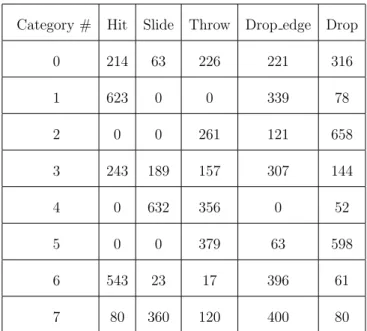
Table 2.1: Distribution of number of videos with specific actions per category. These videos were categorized by participants to 8 different categories and for each category 1040 videos were selected randomly to be used as input data for the deep neural network model.

Category # Hit Slide Throw Drop edge Drop 0 214 63 226 221 316 1 623 0 0 339 78 2 0 0 261 121 658 3 243 189 157 307 144 4 0 632 356 0 52 5 0 0 379 63 598 6 543 23 17 396 61 7 80 360 120 400 80

various viewpoints helped our data-set to be diverse which in turn would help the DNN model to generalize better.

2.2 Behavioral Test

In order to label the animations based on human perception we first needed to know how many categories we can expect from subjects to classify the anima-tions. Experiment 1 was designed to investigate how many distinct categories were needed to classify the animations. Experiment 2 was designed in order to categorize all remaining animations based on categories found in Experiment 1.

(25)

2.2.1 Experiment 1

In experiment 1 a subset of the pool of animations was used in order to under-stand the quantity and the quality of the categories necessary to classify these animations based on human perception and to see how humans group different materials together. The match-to-sample paradigm was utilized in which a grid of 3 × 3 animations was presented as shown in Fig 2.2. One animation was shown in the middle as the target stimuli and eight surrounding animations were tested against it. All animations in this subset were used both as target and test stimuli. Participants needed to select all the surrounding animations that they thought had the same material as the animation located in the center of the grid. A total number of 18 participants were asked to classify the animations based on the perceived material properties and irrespective of the possible similarities in the type of action or the point of view in animations. The k-means clustering method was used to analyze the responses. We calculated the Sum of Squared Errors (SSE) for each k. By plotting the SSE against the number of clusters, we could find a point where adding more clusters does not substantially decrease the SSE, this point is called the elbow point and it is one of the methods used to find out the optimal number of clusters for k-means clustering. k-means clustering and using elbow method resulted in 8 different perceptual categories chosen by participants.

2.2.2 Experiment 2

In experiment 2, in order to categorize all remaining animations, the same ex-perimental set up as Experiment 1 was used (Fig 2.2). In this experiment, the closest animations to the centroids of the 8 categories from experiment 1 were used as the target animation in the middle and all the remaining animations were shown as the test stimuli in the surrounding places of the grid. A total number of 21 participants were similarly asked to choose all animations that had the same material as the target animation in the center. Both Experiment 1 and Exper-iment 2 were conducted in Justus-Liebig-Universit¨at Gießen (by Dr. Alexandra

(26)

Figure 2.2: The behavioral test set-up in Experiment 1 and Experiment 2. The target stimuli was shown in the middle and the test animations were show in the surrounding spots.

Table 2.2: Number of animations in each perceptual category.

Category # 1 2 3 4 5 6 7 8

Number of animations 2799 2000 1280 2640 4640 2720 2440 1040

C. Schmid). Experiment 1 and 2 resulted in having 8 categories of animations that were classified based on human perception. The number of videos per cate-gory is shown in Table 2.2. Now, these classified animations with the appropriate perceptual labels could be fed into a deep convolutional neural network in order to compare its performance to the humans.

(27)

2.3 3D-Convolutional Neural Network Model

2.3.1 Data Preparation

Each animation was 512 × 512 pixels and had 24 frames. In order to feed the an-imations to the DNN model, we resized the anan-imations to 128 × 128 pixels which preserved the spatial and temporal features in the animations while enabling us to fit the model and data in computer memory. In addition, since our anima-tions were simulated in a black and white environment and were not carrying any color-related information, we used only one of the RGB channels of images that the animations were made up of in order to prevent redundancy and preserve memory space. Individual frames of the animations were normalized (using Min-Max normalization) and the pixel values were transformed from (0, 255) range to (0, 1) range which is appropriate as the input for DNNs.

We wanted to use a symmetric data-set for the DNN model in order to prevent biasing it toward a certain category with more data, therefore, we randomly chose 1040 animations from each category which is the minimum number of animations per category among all categories. This resulted in having a total number of 8320 animations for training, validating, and testing the DNN model. We first shuffled the data and then split the data into three parts: 60% for training, 20% for validation, and the remaining 20% for testing the DNN model.

2.3.2 DNN Architecture

Many deep neural network models have been proposed for video classification, action recognition, and generally extracting spatiotemporal features from videos. For example; Two-Stream Convolutional Networks [38] uses two streams of con-volutional neural networks (spatial ConvNet and temporal ConvNet) in order to capture spatial and temporal information separately and then fuses the ex-tracted features in the final layer, LSTM (Long Short Term Memory) composite

(28)

model [39] which uses the long short term memory networks and unsupervised learning algorithms and it has been shown that it improves the classification of human action recognition videos. Other methods include Early Fusion, Late Fu-sion, and Slow Fusion methods [12], LRCN (Long-term Recurrent Convolutional Networks) [13], LSTM, and convolutional temporal feature pooling models [14]. Another deep neural network model for extracting the spatiotemporal information is 3D-Convolutional Neural Network model(3D-CNN) [15] which outperforms all of the above-mentioned models in human action recognition on UCF101 data-set [15, 40].

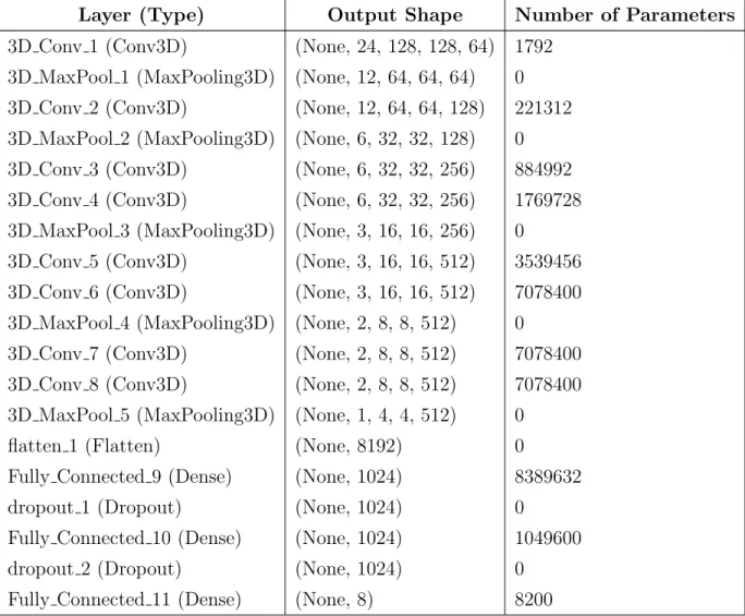
I created a 3D-CNN model similar to the above-mentioned model (which is called C3D model in the original paper [15]) with some minor adjustments. The architecture that has been used in 3D-CNN model is shown in Table 2.3. The animations were fed into the 3D-CNN model in groups of 32 which is called a batch. In Table 2.3 all the “None”s represent the number of animations in a batch which is 32 in this case. The input is a tensor with the shape (32, 24, 128, 128, 1) which are (batch size, number of frames, frame height in pixels, frame width in pixels, number of channels) respectively. The output shapes in Table 2.3 are organized in (batch size, number of frames, frame height in pixels, frame width in pixels, number of filters in that layer) respectively. In each layer, the input is convolved with a 3 × 3 × 3 tensor which is called a filter and then added to a constant called bias. A filter basically is a tensor with weights which are initialized randomly in the beginning. As each batch of inputs passes through the network the weights are changed and optimized based on the current state of the network in order to perform better and minimize the error. Each filter has some weights (in this case 27) and one bias, which are all variables. All weights and biases for different filters in a layer are the parameters of that layer. In the first layer, the network has a 3D-Convolution layer (3D Conv 1) with 64 filters and 1792 parameters. After the first layer, we have a 3D-Max Pooling layer which shrinks the input data by receiving a 3 × 3 × 3 tensor and passing the maximum element between 27 inputs, in this way the 3D-Max Pooling layer shrinks the data by the factor of 9. Since it is just a mathematical function and operation applied to data it has no parameters to be learned. The second

(29)

layer is similar to the first layer in architecture and just the number of the filters is increased from 64 to 128 in the second layer. In layer 3 and 4 we have two convolutions successively because we do not want to use 3D-Max Pooling layer too much. Using 3D-Max Pooling shrinks the data in the spatial and temporal domains in the early layers, however, we do not want that to happen, we want to use the spatial and temporal data as much as we can. Layers 5 and 6 are placed successively and have similar architectures and also layers 7 and 8 are similar in the architecture. In layer (flatten 1) we just flatten the output of the previous layer which means converting the data into a big vector and then we use three consecutive Fully Connected layers after that. Convolutional layers have extracted many spatial and temporal features and we use Fully Connected layers in order to enable the network to choose and combine these features to maximize the performance. We also use two Drop Out layers in order to help the network to generalize better. In Drop Out layers, some percentage (in this network 50%) of the neurons are randomly turned off in order to let all the neurons to learn and generalize better. Overall, there are 37,099,912 trainable parameters in this deep neural network model as shown in Table 2.3.

In addition to the regular animations which are temporally consistent. I shuf-fled the frames of the animations to create temporally inconsistent animations and trained the same 3D-CNN network using these animations. In this situation, there is no useful temporal information in the animations that the convolutional neural network can use to extract features useful for categorization task. The spatial features are present but since the frames are randomly shuffled for each animation, the temporal information acts as noise and contains no useful infor-mation. The results from this training set will be compared to the results of the regular animations in order to investigate the importance of the temporal information in categorizing material animations.

(30)

Table 2.3: DNN Architecture, shape of the tensors, and the number of parameters for each layer.

Layer (Type) Output Shape Number of Parameters

3D Conv 1 (Conv3D) (None, 24, 128, 128, 64) 1792 3D MaxPool 1 (MaxPooling3D) (None, 12, 64, 64, 64) 0

3D Conv 2 (Conv3D) (None, 12, 64, 64, 128) 221312

3D MaxPool 2 (MaxPooling3D) (None, 6, 32, 32, 128) 0

3D Conv 3 (Conv3D) (None, 6, 32, 32, 256) 884992

3D Conv 4 (Conv3D) (None, 6, 32, 32, 256) 1769728

3D Conv 5 (Conv3D) (None, 3, 16, 16, 512) 3539456

3D Conv 6 (Conv3D) (None, 3, 16, 16, 512) 7078400

3D Conv 7 (Conv3D) (None, 2, 8, 8, 512) 7078400

3D Conv 8 (Conv3D) (None, 2, 8, 8, 512) 7078400

flatten 1 (Flatten) (None, 8192) 0

Fully Connected 9 (Dense) (None, 1024) 8389632

dropout 1 (Dropout) (None, 1024) 0

Fully Connected 10 (Dense) (None, 1024) 1049600

dropout 2 (Dropout) (None, 1024) 0

(31)

Chapter 3 Results

3.1 Behavioral Results

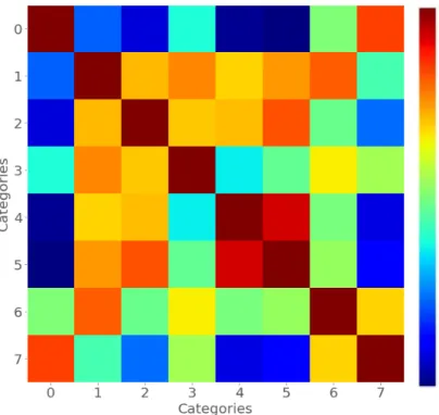
In Experiment 2, participants classified the animations based on their material properties and we used the results to form a confusion matrix for the 8 perceptual categories. The confusion matrix of the behavioral test which was performed by the participants is shown in Fig 3.1. The confusion matrix shows that some categories were almost exclusively mistaken by each other (like category # 0 and category # 7) while some other categories were almost equally confused with other categories (like category # 1, #2, # 3, and # 6) and category # 4 and # 5 were also like those but also heavily mistaken by each other. This result shows that the participants’ perception of material properties were not consistent with each other and there were large individual differences.

3.2 Deep Neural Networks Results

I trained the deep convolutional neural network with 60% of the data as the training set and monitored the training using 20% of the data called validation

(32)

Figure 3.1: The confusion matrix of the behavioral test. Dark red colour shows perfect correlation and dark blue shows zero correlation.

set and finally tested the network using the remaining 20% of the data which is called test set. Each epoch is when the entire training data is passed through the deep neural network model. In order to figure out how many epochs I need to train the network, I trained the network for 50 epochs and monitored the training and validation loss and accuracies. As it is shown in Fig 3.2, it turns out that after 16 epochs the training loss keeps decreasing but the validation loss stops decreasing and then increases which could be considered as a sign of overfitting. Overfitting happens when the networks learn the training data but it is not able to generalize over the test data, it almost remembers the training data too much that decreases its accuracy for the test data (Fig. 3.3). During the training, the network tries to minimize the loss function that has been defined for it. I have used cross-entropy loss function which means that for example if the animation is labeled as category # 0 and the label is [1, 0, 0, 0, 0, 0, 0, 0] the output is the respective probabilities for the categories that network thinks the animation belongs to. So the output would be something like [0.9, 0, 0.05, 0, 0.5, 0.1, 0, 0] and the network will try to minimize the distance between its output and the

(33)

Figure 3.2: Training and validation loss for 50 epochs.

true label of the animation. The cross-entropy loss function is calculated by the formula in Equation 3.1 where N is the number of categories, yi is the correct labels and pi is the probability which is assigned for each class by the deep neural network. Loss = − N X i=1 yilog(pi) (3.1)

We found out that after 16 epochs, overfitting happens. So we trained the network for only 16 epochs in order to obtain the final accuracy of the model. The final accuracies are shown in Table 3.1.

In classification, when the condition is present and the model detects the con-dition we call it the True Positive (TP). True Negative (TN) is when the concon-dition is absent and the model does not detect the condition. False Positive (FP) is when the condition is absent and the model detects the condition. False Negative (FN) is when the condition is present and the model does not detect the condition. In Table 3.1, the precision is the ratio in Equation 3.2.

T P

(T P + F P ) (3.2)

(34)

Figure 3.3: Training and validation accuracy for 50 epochs.

a sample that is negative. The recall is the ratio in Equation 3.3.The recall is intuitively the ability of the classifier to find all the positive samples.

T P

(T P + F N ) (3.3)

The support is the number of animations of each class in the test set which was the 20% of the data chosen randomly. The formula for the F1 score is shown in Equation 3.4.

F 1 = 2 ×(precision × recall)

(precision + recall) (3.4)

It is worth mentioning that we have used a shallower neural network in or-der to categorize the animations. The network had only two convolutional, two max-pooling and two fully connected layers and reached 80% accuracy which is comparable to but lower than the 3D-CNN network that we have used here. The main reason that we used a deeper network is because the C3D model is claimed to be one of the best architectures to extract the spatio-temporal features in videos [15].

(35)

Table 3.1: Classification Report After 16 Epochs when 3D-CNN model is trained and tested using regular animations.

Category # Precision Recall F1-score Support

0 0.89 0.89 0.89 225 1 0.80 0.81 0.81 225 2 0.95 0.96 0.96 193 3 0.91 0.87 0.89 214 4 0.95 0.95 0.95 191 5 0.86 0.92 0.89 170 6 0.88 0.81 0.84 227 7 0.82 0.86 0.84 219

3.3 Comparison

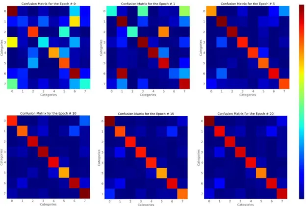
The confusion matrix of the 3D-CNN model results in Fig 3.4 shows that as the 3D-CNN model trains more and more on the data its decisions become more and more certain.

In order to compare the confusion matrix of behavioral experiment shown in Fig 3.1 with the confusion matrices of the DNN model predictions during the training which are shown in Fig 3.4, we used the Spearman Correlation coeffi-cient. Spearman Correlation coefficient is a metric to measure the monotonic relationship between two variables. Monotonic relationship means that when a variable increases the other variable either only increase or only decreases. The Spearman Correlation coefficient is a number between -1 and +1. If it is closer to +1 it means that the variables have a strong positive correlation, closer to 0 means no correlation and closer to -1 means strong negative correlation.

(36)

Figure 3.4: Confusion Matrix for the DNN model during training, the Epoch 0, Epoch 1, Epoch 5, Epoch 10, Epoch 15, Epoch 20.

(37)

Figure 3.5: Spearman Correlation for the temporally consistent animations

test and 3D-CNN model during 20 epochs is presented in Fig 3.5, and their p-values are shown in Fig. 3.6. These results show that in the beginning when the network has just trained on the data once (Epoch 0) there is a moderate correla-tion between the behavioral and the 3D-CNN results which shows that 3D-CNN learns very quickly even after just one epoch. As the number of epochs goes up and the 3D-CNN model trains more on the data the correlation goes up to 0.74 which is considered a strong correlation which means that the performance of the 3D-CNN model slowly becomes more and more similar to that of humans. However, after some time (after Epoch 15) the Spearman Correlation coefficient starts to drop, probably because the performance of the 3D-CNN becomes more and more certain. Even though the accuracy of the network is not increasing from Epoch 15 to Epoch 20 but since it is training on the data more, the net-work’s decisions become more certain. For example if the correct label was [1, 0, 0, 0, 0, 0, 0, 0] and the networks response was [0.9, 0, 0.05, 0, 0.5, 0.1, 0, 0], the probabilities change and the response becomes more certain like [0.99, 0, 0, 0, 0, 0.01, 0, 0], therefore the correlation decreases while the accuracy of the network remains almost the same. Based on this result we can say that the conventional training and testing routine for the deep neural network models are not necessar-ily creating models that perform similar to humans. Even if we control the deep

(38)

Figure 3.6: P-value of Spearman Correlation for the temporally consistent ani-mations

neural networks to prevent overfitting the best performance of the model is not necessarily the best state of the network to be compared to humans. Especially in this case that humans have more varied responses and they probably perceive material properties in different ways. Also, the deep neural networks have very good memories compared to humans and have access to all the data and they go through the data many times in order to learn it so they will make more certain decisions about the category of the animations compared to the population of humans with probably various perceptual skills.

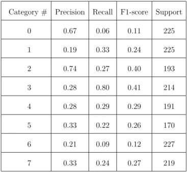
This 3D-CNN network was trained on regular and temporally consistent an-imations, but we wanted to see how this model would perform if we test it by temporally inconsistent animations whose frames were shuffled randomly. The accuracy became only 28% and it dropped dramatically compared to accuracy of testing on regular animations as expected. The classification report for this test is shown in Table 3.2. The 3D-CNN model that has been trained on regu-lar animations extracted some spatial and temporal features that have temporal consistency and when we test it using shuffled animations the extracted features are not really useful.

(39)

Previously, we fed the same animations with 64 × 64 size to the same 3D-CNN model. We found out that the accuracy became 81% which is lower compared to the condition in which the animations had 128 × 128 size. It seems that by resizing the animations to 64 × 64 we are definitly loosing some spatial features that are useful for the categorization.

Table 3.2: Classification Report After 16 Epochs when 3D-CNN model is trained using regular animations but tested using the temporally inconsistent animations.

0 0.67 0.06 0.11 225 1 0.19 0.33 0.24 225 2 0.74 0.27 0.40 193 3 0.28 0.80 0.41 214 4 0.28 0.29 0.29 191 5 0.33 0.22 0.26 170 6 0.21 0.09 0.12 227 7 0.33 0.24 0.27 219

3.3.1 Temporally Inconsistent Animations

In order to investigate how temporal information contributes to the accuracy of the deep neural network model, we trained the model using the temporally inconsistent input. We shuffled the frames of the animations randomly in order to disrupt the consistency and the sense of regular motion in the animations. The 3D-CNN network similarly was trained on temporally inconsistent animations. It reached 77% accuracy after 16 epochs which is comparable to 85% accuracy of the 3D-CNN trained on regular animations. The loss and accuracy for the training and validation sets are shown in Fig 3.7 and Fig 3.8 respectively. The performance

(40)

Figure 3.7: Training and validation loss for 50 epochs when 3D-CNN model is trained using the temporally inconsistent animations.

was just a little bit poor than the regular condition. The Spearman Correlation coefficient for this model in comparison with the behavioral results are shown in Fig 3.9 which shows that in the beginning the Spearman Correlation coefficient is lower compared to the temporally consistent condition which could arise from the fact that because the temporal information is absent, the 3D-CNN model finds it hard to find the minimum of the loss function. However, after some epochs the Spearman Correlation coefficient increases and becomes comparable to that of the temporally consistent condition but unlike that, it remains almost constant until the last epoch. The classification report for the 3D-CNN when it is trained using temporally inconsistent animations is shown in Table 3.3.

This result shows that the 3D-CNN finds a way to classify the material an-imations even if the frames are randomly shuffled and the anan-imations have no temporal consistency. This means that at least for the 3D-CNN model the tem-poral information has less value compared to spatial information in categorizing the material animations.

When an image is fed to a convolutional neural network, the image is convolved with a filter and results in another image called feature map. That feature map

(41)

Figure 3.8: Training and validation accuracy for 50 epochs when 3D-CNN model is trained using the temporally inconsistent animations.

then is treated as an input for the filter of the next layer, it will be convolved with the filter in the next layer and the result will be the feature map of the second layer. The feature maps of the 3D-CNN network for the first 8 layers of the network for one specific example are shown in Fig 3.11 to Fig 3.23. As we can see in Fig 3.11 and Fig 3.13 the filters in the early layers are responsive to lines and corners and extract very primitive features from the object and the scene. As we go deeper in the network (Fig 3.15 and Fig 3.16) it seems like the filters are extracting more complex features and they encompass all the object and their receptive field increases. Apart from that, it is also clear that since the data is temporally shrunken the filters extract the temporal features and motion of the object. In Fig 3.17, Fig 3.18, and Fig 3.19 we see that the feature maps become more sparsely active and the filters are more responsive to specific areas like places that object deformations occur in the animation (specifically in Fig 3.17) instead of concentrating on the whole object. As we go to the deeper lay-ers as shown in Fig 3.19 up to Fig 3.23 successive 3D-Convolutions and 3D-Max Poolings in previous layers have shrunken the data in both temporal and spatial domain and we cannot recognize the shape or motion of the object anymore. The feature maps are just sparsely activated, which is enough to collect and combine

(42)

Figure 3.9: Spearman Correlation when 3D-CNN model is trained using the temporally inconsistent animations.

the necessary key features in order to predict the correct category of the material animations. The color code for these figures is shown in Fig 3.12.

(43)

Figure 3.10: P-value of Spearman Correlation when 3D-CNN model is trained using the temporally inconsistent animations.

3.3.2 Intermediate Layers

In order to see how each layer contributes to the categorization of the anima-tions, we used t-Distributed Stochastic Neighbor Embedding (t-SNE) method to visualize the clusters of the outputs of the intermediate layers.t-SNE is a dimen-sionality reduction technique that receives a high dimensional data and outputs a 2 dimensional or 3 dimensional data that is more suitable for visualization. We randomly chose 300 animations from the test data and feed them to the 3D-CNN model. The outputs of each layer reshaped to a big one-dimensional vector and then t-SNE was applied to the respective outputs of each layer. The t-SNE visu-alization for all layers are shown in Fig 3.24 - Fig 3.39 in which x-axis and y-axis are the two dimensions that the outputs of the layers are reduced to. Each point represents one of those 300 animations and color-coding in the legend shows the respective category of each animation. In Fig 3.24 we can see that the represen-tation of the output of the first layer is totally unorganized and animations from all categories are mixed. The situation is the same for the next couple of layers but we can see that in Fig 3.31 and Fig 3.32 many animations especially from category #2, category #5 and category #6 are starting to group together.Later

(44)

Table 3.3: Classification Report After 16 Epochs when 3D-CNN model is trained using the temporally inconsistent animations.

0 0.73 0.82 0.77 225 1 0.73 0.64 0.68 225 2 0.87 0.90 0.88 193 3 0.85 0.70 0.76 214 4 0.80 0.91 0.85 191 5 0.77 0.80 0.78 170 6 0.72 0.79 0.76 227 7 0.73 0.67 0.70 219

in Fig 3.34, Fig 3.35 and Fig 3.36 we can see that category #2, category #4, category #6, and category #3 are becoming more distinct. In Fig 3.37 and Fig 3.38 it is shown that all categories are becoming distinct and separated, and those categories that were already distinct like category #2 increasing their distance from other categories. In Fig 3.39 we can see that all categories are distinguish-able and separdistinguish-able. However, in all layers, there are some outliers which are due to representing a high-dimensional data in two dimensions and also due to the imperfection of the 3D-CNN classification.

(45)

Figure 3.11: Feature map of layer 1 after 3D-Convolution. 25 sample feature maps of the first layer are shown. Each feature map is 128 × 128 which is the size of the output of the first layer. In each feature map dark purple shows zero response of the respective filter and yellow shows the highest response.

Figure 3.12: The color code for the Fig 3.9 to Fig 3.21. According to this color code, dark purple shows zero response of the filter and yellow shows the highest response.

(46)

Figure 3.13: Feature map of layer 1 after 3D-MaxPooling. Here we can see that the dimension have become 64 × 64 which is the dimension of the output of the first layer after 3D-Max pooling. We can see that the filters are responsive to edges and corners of the object.

(47)

Figure 3.14: Feature map of layer 2 after 3D-Convolution. We can see that because of temporal convolution and max pooling in the time dimension, feature maps are showing some sense of motion compared to previous layer.

(48)

Figure 3.15: Feature map of layer 2 after 3D-MaxPooling.Here because of the max pooling which shrinks the input in time domain, we cans see that feature maps are responsive to multiple frames and showing motion.

(49)

Figure 3.16: Feature map of layer 3 after 3D-Convolution. We can see that some filters are responsive to the whole object in this layer.

(50)

(51)

Figure 3.18: Feature map of layer 4 after 3D-MaxPooling. Max pooling shrinks the data in spatial and temporal domains and in this layer information from multiple frames are extracted and therefore we cannot see the actual shape of the object anymore.

(52)

(53)

Figure 3.20: Feature map of layer 6 after 3D-Convolution. Here the feature map is activated sparsely and all temporal and spatial features of the animations are collapsed because of the convolutions and max poolings in the network.

(54)

(55)

(56)

Figure 3.23: Feature map of layer 8 after 3D-Convolution. Here the feature map is sparsely activated, but this is useful because these few activations are actually contributing to determine the final label of the animation.

(57)

(58)

(59)

(60)

(61)

(62)

(63)

(64)

(65)

(66)

(67)

(68)

(69)

(70)

(71)

(72)

(73)

Chapter 4 Discussion

4.1 What We Have Found?

By comparing the performance of 3D-CNN with that of humans in categorizing the material animations, we found that the conventional maximum training of the neural network is not necessary to capture the most similar performance of the neural network to humans. In fact, the similarity of the performance of the 3D-CNN model to humans grows as we train the model but it reaches its peak and then starts to deviate from the human behavior as we train the network to reach the maximum prediction power based on Fig 3.5. The reason is that humans make more diverse decisions based on their prior experiences however the 3D-CNN model acts as a single entity and reaches more and more solid deci-sions as we train it and feed more data. In addition, the 3D-CNN model iterates through the whole data again and again which is probably more than pre-training time which was dedicated to participants to familiarize themselves with the ma-terial categories, therefore, the 3D-CNN model makes almost perfect judgments and is not as prone to error as humans. This shows that if we want to create a deep neural network model and compare it with humans in any level maybe the conventional training of the deep neural network models which is only restricted by overfitting to the training data is not the best way to go.

(74)

Also, by training the 3D-CNN on regular, temporally consistent animations and also training it on the temporally inconsistent animations and comparing the results we found out that the 3D-CNN model can use spatial information alone in order to categorize the material animations. So for the 3D-CNN model, the temporal information in the animations are not critical for inferring the material properties and categorizing the materials. However, further studies should be conducted in order to investigate the importance of temporal consistency of the animations for humans in the material categorization task.

Previously, we built a 2D-CNN model that was receiving only one frame of the animations and was trained to categorize them. The 3D-CNN performed rel-atively better than the 2D-CNN. By comparing the performance of the 2D-CNN model and 3D-CNN model we thought that the motion is an important factor in evaluating the material properties of the objects in the 3D-CNN model. How-ever, the number of parameters in 2D-CNN and 3D-CNN were not similar which makes it unfair to expect similar results from them in the first place. Therefore, in the current model, we used only 3D-CNN model and instead of building dif-ferent 2D architecture for the deep neural network we tried to manipulate the temporal consistency of the input in order to investigate the importance of the motion information in material categorization.

4.2 Implications of the study

The extrapolation of this study to future could result in creating a model that can differentiate between several different material properties in different condi-tions(e.g. illuminations) and can infer the mechanical properties of the objects by looking at the movies of the objects. Such a model fed with the prior information from the real world materials could be used in several different industries such as self-driving cars. For example, the speed of the car could be controlled if some

(75)

part of the road is shiny and wet and therefore (possibly) slippery or if there is an obstacle in a road it could be a white colored (or illuminated) rock or it could be just a clump of white paper on the road, if the artificial intelligence installed on the self-driving car is able to differentiate between this two situations it may make very different decisions that could save lives.

4.3 Limitations

It should be considered that the task performed by humans and the 3D-CNN model is not exactly the same. A grid of 9 animations was presented to humans and they decided which of the surrounding animations have the same material as the animation displayed at the center of the grid. However, the 3D-CNN model is just observing one animation at a time and decides which of the eight categories it belongs to. Also, the model has the chance to observe all animations 16 times, however, humans had a limited amount of time to familiarize themselves with the animations and the material categories. Therefore, comparing human performance with the performance of the 3D-CNN model might not be the fairest comparison.

4.4 Future Directions

One of the future directions could be using point-light animations in order to bet-ter investigate the importance of motion in the evaluation of mabet-terial properties. Using point-light material animations as a training set and full animations as a test set and vice versa could help to understand this. Some frames of the point light stimuli are shown in Fig 4.1.

The other question that is worth exploring is that if the 3D-CNN works fine even when the animations are temporally shuffled, how humans would perform if

(76)

Figure 4.1: Point-light stimuli.

we ask them to categorize the temporally inconsistent material animations.

Another possibility would be using eye-tracking and comparing the attention maps of humans and machines, to see how similar they attend in order to infer the material properties of the objects. Also, making a more biologically plausible deep neural network model (possibly with separate ventral and dorsal streams) and comparing the activation in different layers of the deep neural network model with the activation of different levels of the visual cortex would be another interesting possibility.

4.5 Conclusion

This study showed that the 3D-CNN model can successfully categorize the ma-terial animations that are labeled based on human perception and reach high accuracies. Also, we showed that the regular routine training of the deep neural network may not necessarily be the best state of the network to be compared against humans, it certainly is not the closest to human performance in case of 3D-CNN and material animation categorization task. Additionally, we found that 3D-CNN can categorize the material animations even if their frames are randomly shuffled and the temporal information in material animations are not critical features for the 3D-CNN in categorizing material animations. In the case

(77)

of temporally inconsistent animations, 3D-CNN can rely solely on the spatial fea-tures of the material animations and reach almost the same performance as the temporally consistent condition.

(78)

Bibliography

[1] M. Hematinezhad, M. H. Gholizadeh, M. Ramezaniyan, S. Shafiee, and A. G. Zahedi, “Predicting the success of nations in asian games using neural net-work.,” Sport Scientific & Practical Aspects, vol. 8, no. 1, 2011.

[2] W. S. McCulloch and W. Pitts, “A logical calculus of the ideas immanent in nervous activity,” The bulletin of mathematical biophysics, vol. 5, no. 4, pp. 115–133, 1943.

[3] F. Rosenblatt, “The perceptron: a probabilistic model for information stor-age and organization in the brain.,” Psychological review, vol. 65, no. 6, p. 386, 1958.

[4] M. Minsky and S. Papert, “An introduction to computational geometry,” Cambridge tiass., HIT, 1969.

[5] R. Hecht-Nielsen, “Theory of the backpropagation neural network,” in Neu-ral networks for perception, pp. 65–93, Elsevier, 1992.

[6] R. M. Cichy, A. Khosla, D. Pantazis, A. Torralba, and A. Oliva, “Comparison of deep neural networks to spatio-temporal cortical dynamics of human visual object recognition reveals hierarchical correspondence,” in Scientific reports, 2016.

[7] S. Lawrence, C. L. Giles, A. C. Tsoi, and A. D. Back, “Face recognition: a convolutional neural-network approach,” IEEE transactions on neural net-works, vol. 8 1, pp. 98–113, 1997.

(79)

[8] C. Szegedy, A. Toshev, and D. Erhan, “Deep neural networks for object detection,” in NIPS, 2013.

[9] A. Krizhevsky, I. Sutskever, and G. E. Hinton, “Imagenet classification with deep convolutional neural networks,” Commun. ACM, vol. 60, pp. 84–90, 2012.

[10] S. Ji, W. Xu, M. Yang, and K. Yu, “3d convolutional neural networks for human action recognition,” IEEE Transactions on Pattern Analysis and Ma-chine Intelligence, vol. 35, pp. 221–231, 2010.

[11] H. Adeli and G. J. Zelinsky, “Learning to attend in a brain-inspired deep neural network,” CoRR, vol. abs/1811.09699, 2018.

[12] A. Karpathy, G. Toderici, S. Shetty, T. Leung, R. Sukthankar, and L. Fei-Fei, “Large-scale video classification with convolutional neural networks,” in Proceedings of the IEEE conference on Computer Vision and Pattern Recog-nition, pp. 1725–1732, 2014.

[13] J. Donahue, L. Anne Hendricks, S. Guadarrama, M. Rohrbach, S. Venu-gopalan, K. Saenko, and T. Darrell, “Long-term recurrent convolutional networks for visual recognition and description,” in Proceedings of the IEEE conference on computer vision and pattern recognition, pp. 2625–2634, 2015. [14] J. Yue-Hei Ng, M. Hausknecht, S. Vijayanarasimhan, O. Vinyals, R. Monga, and G. Toderici, “Beyond short snippets: Deep networks for video classifica-tion,” in Proceedings of the IEEE conference on computer vision and pattern recognition, pp. 4694–4702, 2015.

[15] D. Tran, L. Bourdev, R. Fergus, L. Torresani, and M. Paluri, “Learning spatiotemporal features with 3d convolutional networks,” in Proceedings of the IEEE international conference on computer vision, pp. 4489–4497, 2015. [16] M. F. Stollenga, J. Masci, F. Gomez, and J. Schmidhuber, “Deep networks with internal selective attention through feedback connections,” in Advances in neural information processing systems, pp. 3545–3553, 2014.

Comparing the performance of humans and 3D-convolutional neural networks in material perception using dynamic cues

COMPARING THE PERFORMANCE OF

HUMANS AND 3D-CONVOLUTIONAL

NEURAL NETWORKS IN MATERIAL

PERCEPTION USING DYNAMIC CUES

a thesis submitted to

the graduate school of engineering and science

of bilkent university

in partial fulfillment of the requirements for

the degree of

master of science

in

neuroscience

By

Hossein Mehrzadfar

July 2019

ABSTRACT

COMPARING THE PERFORMANCE OF HUMANS

AND 3D-CONVOLUTIONAL NEURAL NETWORKS IN

MATERIAL PERCEPTION USING DYNAMIC CUES

¨

OZET

˙INSANLARIN PERFORMANSINI KARS¸ILAS¸TIRMAK

VE 3D-KONVOLEKS˙IYONEL N ¨

ORAL A ˘

GLARDA

D˙INAM˙IK P˙IS

¸ ˙IRME KULLANILAN MALZEME

ANLAYIS

¸I

Acknowledgement

Contents

List of Figures

List of Tables

Chapter 1

Introduction

1.1

Purpose of The Study

1.2

Deep Neural Network Models

1.2.1

What is a Deep Neural Network?

1.2.2

The Convolutional Neural Networks

1.2.3

Deep Neural Networks in Vision

1.3

Material Motion Perception

1.3.1

Material Perception

1.3.2

Material Dynamics

1.4

Research Question and Hypothesis

Chapter 2

Materials and Methods

2.1

Material Animations

2.2

Behavioral Test

2.2.1

Experiment 1

2.2.2

Experiment 2

2.3

3D-Convolutional Neural Network Model

2.3.1

Data Preparation

2.3.2

DNN Architecture

Chapter 3

Results

3.1

Behavioral Results

3.2

Deep Neural Networks Results

3.3

Comparison

3.3.1

Temporally Inconsistent Animations