Coding of speech and image signals using Gabor decomposition

гг rs ■; ν'·, 'i ^ ^ *’· ? ". i • :,y| í ,;r '^ .P'·,’^ ^;; r-‘ ¿^'■■.'': · .•^.İJıTİ j_{<«·».ίί-ъ'чи^} |H è |r¿ ._{S Ü kÍM<^ ilÉlk\^.'} ι-Τ;4:ΤΤ!»ν^ Τ'*·ΐ''’«

2

'^ ' ' * -- '· ^ M * . 1 W *«·' İ M Mi.'.. Ί W MM "Τ '- T Г'· '"::? ...т г ‘·

/7 ,·

ГА Г

7 В ё Л

. S 6 S

6 <В6

/ з э ^

CODING OF SPEECH AND IMAGE SIGNALS USING

GABOR DECOMPOSITION

A THESIS

SUBMITTED TO THE DEPARTMENT OF ELECTRICAL AND

ELECTRONICS ENGINEERING

AND THE INSTITUTE OF ENGINEERING AND SCIENCES

OF BILKENT UNIVERSITY

IN PARTIAL FULFILLMENT OF THE REQUIREMENTS

FOR THE DEGREE OF MASTER OF SCIENCE

By

Emre Gündüzhan

July 1994

ΤΚ: i Ъс

5(

11

I certify that I have read this thesis and that in my opinion it is fully adequate, in scope and in quality, as a thesis for the degree of Master of Science.

Assoc. Prof. Dr. A. Enis Qetin(Principal Advisor)

I certify that I have read this thesis and that in my opinion it is fully adequate, in scope and in quality, as a thesis for the degree of Master of Science.

o m L ·

-Assist. Prof. Dr. Orhan Arikan

I certify that I have read this thesis and that in my opinion it is fully adequate, in scope and in quality, as a thesis for the degree of Master of Science.

Assist. Prof. Dr. Billur Barshan

Approved for the Institute of Engineering and Sciences:

Prof. Dr. Mehmet Bfdray

ABSTRACT

CODING OF SPEECH AND IMAGE SIGNALS USING

GABOR DEGOMPOSITION

Emre Gündüzhan

M.S. in Electrical and Electronics Engineering

Supervisor: Assoc. Prof. Dr. A. Enis Çetin

July 1994

A new low bit rate speech coding method which uses Gabor time-frequency decomposition and the matching pursuit algorithm is developed. A new al­ gorithm based on the projections onto convex sets method is used to smooth the discontinuities between speech frames. A two-dimensional extension of the Gabor time-frequency decomposition is also developed for image coding. Simulation examples are presented.

Keywords: Speech coding, image coding, time-frequency dictionaries, match­ ing pursuit algorithm.

ÖZET

GABOR AÇILIMI KULLANARAK SOZ VE İMGE

SİNYALLERİNİN KODLANMASI

Emre Gündüzhan

Elektrik ve Elektronik Mühendisliği Bölümü Yüksek Lisans

Tez Yöneticisi: Doç. Dr. A. Enis Çetin

Temmuz 1994

Gabor zaman-sıklık açılımı ve karşılaştırmalı takip algoritması kullanılarak yeni bir az bitle söz kodlama tekniği geliştirildi. Söz çerçeveleri arasındaki süreksizliğin azaltılması için içbükey kümeler üzerine izdüşüm tekniğine dayanan yeni bir algoritma kullanıldı. Gabor zaman-sıklık açılımının iki boyuta genellemesi yapıldı ve imge kodlama için kullanıldı. Benzetim çalışmaları yapıldı.

Anahtar kelimeler : Söz kodlama, imge kodlama, zaman-sıklık sözlükleri, karşılaştırmalı takip algoritması.

ACKNOWLEDGMENT

I would like to thank Assoc. Prof. Dr. A. Enis Çetin for his supervision, guidance, suggestions and encouragement throughout the development of this thesis.

Contents

1 Introduction 1

1.1 N o ta tio n ...

2

1.2

Time-Frequency Atomic D ecom p osition s... 3 1.3 Matching Pursuit in Finite S paces... 3 1.4 Matching Pursuit with Gabor Time-Frequency Dictionaries . . .

6

2 Speech Coding 9

2.1

Reducing Discontinuities Using the Method of Projections Onto Convex S e t s ...

12

2.2

Simulation E x a m p le s... 14 2.3 Computational Complexity of the New Speech Coding Method . 16

3 Image Coding 20

3.1 Simulation E x a m p le s...

22

4 Conclusion 26

List of Figures

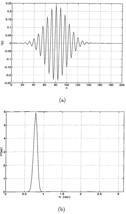
1.1 (a) A discrete Gabor atom with parameters (s,p, k, (j>) = (50,80,25, j ) and length N =

200

and (h) the magnitude of its Fourier trans­ form...

8

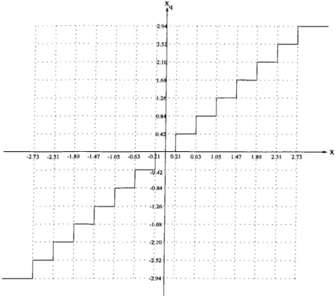
2.1

The 4 bit uniform quantizer used to quantize the angles. 14 2.2 (a) An original speech signal, (b) the signal after coding/decoding

using the Gabor time-frequency decomposition, and (c) the sig­ nal after coding/decoding using an LPC-10 vocoder... 18 2.3 (a) A voiced speech segment, (b) the coded/decoded segment

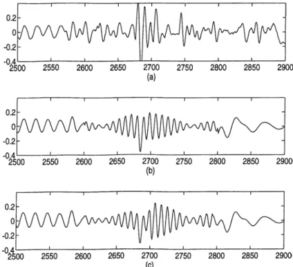
having two discontinuities, and (c) the same segment after ap­ plying the POCS based algorithm twice... 19 2.4 (a) An unvoiced speech segment, (b) the coded/decoded seg­

ment having two discontinuities, and (c) the same segment after applying the POCS based algorithm twice... 19

3.1 The original (a) and the reconstructed (b) Barbara images. . . . 24 3.2 The comparison of the matching pursuit and JPEG algorithms

using the Barbara image... 25 3.3 The comparison of the matching pursuit and JPEG algorithms

using the Lena image. 25

List of Tables

2.1 The 6 hit n-law quantizer used to quantize the inner products. . 15

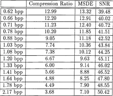
3.1 The compression results for the Barbara image... 23 3.2 The compression results for the Lena image... 23

Chapter 1

Introduction

Signal decompositions over a family of functions are widely used in signal processing. The family of functions used in such a decomposition is called a dictionary. The main advantage of signal decomposition methods is to rep­ resent a given signal by a countable set of coefficients. Most commonly used decompositions are the Short-time Fourier transform (STFT) [

2

], the Wigner- Ville transform [3], and the wavelet transforms [4], [5]. The family of functions in a dictionary are usually linearly independent and they form an orthonor­ mal basis. Using a basis as a dictionary of a decomposition may result in the smallest possible dictionary for the exact reconstruction of the signal, however, it is difficult to extract some time-frequency properties of a signal from such an expansion. For example, the decomposition of signals well localized in time over a Fourier basis or the decomposition of signals having a narrow high- frequency support over a wavelet basis results in a poor representation. These facts motivate decompositions over large and redundant dictionaries. Instead of using a single basis in this thesis we select functions, which are most useful to represent our signal, from a redundant dictionary and decompose the signal over these functions.

Using a large dictionary is especially useful in the representation of a signal whose localization in time and frequency vary widely. In this case using a single basis will not usually be sufficient for a good representation and the dictionary should contain functions which are well-localized both in time and in frequency. The elements of such a dictionary are called the time-frequency atoms. The decomposition of a signal over a redundant dictionary is adaptive. A signal is represented using a chosen subset of the dictionary such that the atoms in the subset are best adapted to the signal properties. There is an algorithm, called the matching pursuit, which can perform such an adaptive decomposition over

families of functions [

1

]. There is a similar algorithm developed by Qian and Chen to expand signals over a time-frequency dictionary [

6

].

In this thesis a time-frequency atom family, called the Gabor dictionary [

1

], is used in speech coding. A low bit rate speech vocoder which uses a time-frequency decomposition is proposed. The same method is also applied to image coding using two-dimensional atoms. In the next section we intro­ duce the time-frequency atoms and the matching pursuit algorithm which are studied in detail in [

1

]. In Chapter

2

, a speech coding method using Gabor time-frequency atoms is described and a new algorithm to smooth the disconti­ nuities between speech frames is developed. Some simulation examples are also given in Chapter

2

. In Chapter 3, two-dimensional Gabor atoms are developed and an image coding algorithm is given. Some simulation results for image coding are also shown in this chapter.

1.1

Notation

Consider the Hilbert space L^(C) of complex valued functions, / , which satisfy / OO

I f{ t) p dt < OO. (1.1)

-OO

For any f , g ^ L^(C ), the inner product is defined by / OO

f{t)g*{t)dt (

1

.

2

)

-OO

where g*{t) is the complex conjugate of g{t). The continuous-time Pburier transform of /

6

li^(C ) is defined by

A 1 poo

m = ^ y_^ /( O e - '- r f i . (1.3)

Let H be the inner product space of complex valued discrete-time functions periodic with N. We define the inner product of f , g EiUhy

N - l

< h g > = f[n\g"[n]. (1.4) n=0

For any a —> 0 (or oo), any quantity that is bounded by a constant times a is denoted by (9(a).

1.2

Time-Frequency Atomic Decompositions

In general, a family of time-frequency atoms can be generated by scaling, shift­ ing, and modulating a window function g{t) G L 2(R ). We assume that g{t) is real, continuously differentiable, has unity norm, and |g[t)

I is O ( ^ ) . A

time-frequency atom is defined by

5'7(0

1

A - u iet

(1.5)

where

7

= (s, u, e) which are the parameters of

7

. The parameter s is a scaling factor, u is a shift term and e is the modulating index. Here

7

is an element of the set r =: R + x R^. The energy of is concentrated in a neighborhood of u, whose time window size is proportional to s. If we take the Fourier transform of both sides in (

1

.

5

) then we get

g^w) = y/sg{s{w - e))e-j[w -e )u (

1

.

6

)

The energy of g.^{w) is concentrated in a neighborhood of e, whose frequency window size is proportional to s “ ^.

The dictionaries in a window Fourier transform and a wavelet transform are special cases of (1.5). In a window Fourier transform the parameter s is fixed, so the time scale does not change [

2

] and in a wavelet transform s and e are inversely proportional to each other [4].

In a time-frequency atomic decomposition the aim is to select a countable subset of atoms (if

7

„(i))neN from the dictionary and express the signal, / ( t ) , as a weighted sum of these atoms, i.e..

/(0

~ O-nd'^nA)· (1.7)

n = 0

In the next section we describe an algorithm, called the matching pursuit, which can carry such a decomposition.

1.3

Matching Pursuit in Finite Spaces

The dictionary used in a time-frequency decomposition is redundant. In order to decompose a signal “optimally” we must choose atoms which best match the signal properties. The matching pursuit algorithm can be used for such an adaptive decomposition.

Let H be a signal space with a finite dimension N. We define a dictionary V = as a family of vectors in H, such that ||=

1

for all

7

G F. Let V be the closed linear span of vectors in T>. We assume that the dictionary T> is complete, i.e., V = H.

Let / e H. We want to get the closest approximation of / in norm by one of the vectors in T>. Clearly, we must choose G T> such that |< f,g.ya >| is maximum. In some cases, it is only possible to find a vector g.y^ satisfying

l< > l> « sup |< f,g^

>1

7GF ,

0

< a <

1

. 7GF

Next, / is decomposed as

/ = <

/,</70

> 9io + where R f is the residual vector. Since g.y^ ± i ? /,

Il/ir= l< /,i, >P + l l « / i r

(

1

.

8

)

(1.9)

(1.10)

The matching pursuit algorithm sub-decomposes the residual vector R f on a vector in T> and this procedure is repeated for each new residual vector. Let = / · Suppose the order residue, i ? " /, was computed for some n >

0

. We choose a vector g^^ G V which satisfies

l< > l> « sup |< R^f,g^

>1

.

7

GF Then, we sub-decompose R ^f into

R - f = < R rf,g ,„

>

+ B”+7

(1.11)

(1.12)

to obtain the (n +

1

)^^ residue. If we carry this decomposition up to the order m, then we obtain an order approximation of / , i.e..

m

—1

(1.13)

n=0

Since _L for all 0 < n < m, we get an energy conservation equation m

—1

Il/|p= ^ |<

>P + II« ” /

(1.14)

n=0

T h e o r e m

1.1

If the dictionary T> is complete then {g.y„)n>o and {R^f)n>o defined inductively by (1.11) and (1-12) satisfy

/ = E < R"f,g^n > 9^u n=0 and for any / G H . (1.15) (1.16) n=0

If we stop the iterations at an order m then the decomposition is given by (1.13). Here, / is approximated with an error equal to However, this approximation is not the best one can achieve using the vectors (fi'-Y„)o<n<m· Let V „i be the span of (.

97

„)o<n<m and Pvm the orthogonal projector on Ym- The closest approximation of / using the vectors in Y ^ is given by

m—1

Pv./ = E <

> 3-r. +

Pv,.fi” /.

(1.17) n=0

In general, the family of vectors {g'f„)o<n<m is not orthogonal. In this case P y ^ R ^ f ^ 0. The computation of

m—1

P v . « ” / = E *»51. (1.18)

n = 0

is called a backprojection. Using backprojection we can decompose / as m — 1

f ^

J2i<

> ■^Xn)g'1n + (1.19)

n= 0

where P w „ , / is the orthogonal projection of / onto the space W ^ , which is the orthogoiicil complement of Ym in H. We have to solve the following linear- system of equations to calculate the coefficients (xn)o<n<m· For any 0 < k < m,

m —

1

^ f'lQik ^ ^ · (1.20)

n=0

If the vectors (i'

7

„)o<n<m are linearly dependent then the solution is not unique, but we can always find a solution.

If the dictionary is very redundant the search for the vector g^^ in (

1

.

11

) can be limited to a sub-dictionary = (fif

7

)

7

er„ C P , where Fq, C F is a finite index set such that for any / € H

sup |< f,g^ >|> a sup |<

/,(/7

>| .

7er«

7

€F

Depending on the dictionary, r „ can be much smaller than F. At each iteration, instead of searching the whole dictionary, we search for a vector gy^ G T>a such that

l< >

1

= sup |< BJ^f,gy

>1

. (

1

.

22

)

7erc

The rest of the algorithm remains the same.

1.4

Matching Pursuit with Gabor Time-Frequency Dic­

tionaries

A time-frequency dictionary is a family of time-frequency atoms defined in (1.5). If a matching pursuit is used with a time-frequency dictionary, then any function / G L^(C) is decomposed into a sum of time-frequency atoms that best match its residues. It has been shown that a time-frequency dictionary is complete in L^(C ) [7]. Therefore, for any / G L^(C) a matching pursuit yields

/ = S < -S“ /.9 7 . > 9 » (1.23)

n=0

where

7

„ = (

5

„ ,u „ ,e „ ) and

. .

1

A — u

5^7n(0 “ ~

If the window function, g{t), is chosen as the normalized Gaussian function (1.24)

g(t) = 2<e-TTi^ (1.25)

then the corresponding family of functions {gy)y^r is called the Gabor time- frequency dictionary.

In practice the matching pursuit algorithm has to be used in discrete-time. We suppose that we want to decompose a real discrete-time signal with N samples. Our vector space H is the set of all discrete signals periodic with N. The window function is again the normalized Gaussian given by (1.25). For each scale s we sample the window function and periodize it over N points to get

9

.W = ^ E

9

( ^ ^ ^ ) (1-26) where Kg normalizes the discrete norm of gg. Then, for any integers 0 < p < N — 1 and

0

< f c < A ^ —I we denote

7

= (s,p, ^ ) and define the corresponding discrete complex Gabor atom as

Since we want to decompose a real signal, we must use real time-frequency atoms to get real expansion coefficients. For any

7

= {s,p, and a phase 4> G [

0

, 27t) the real discrete time-frequency atoms are given by

27T k

«1,♦)['>] =

- p|

+ <t>)

(1.28) where is the normalization constant to make || ||= I. The normal­ ization constant is given by

^^(

7

.

0

) =

yi -t-

Real{e^^'t’ < g^,g* > } (1.29)

For each

7

= (

5

,p, and phase the real and complex discrete atoms are related by

5

^(

₇

, [ n

{e>’^g^[n]+e ^ V [n ]).

2

(1.30)

A real discrete Gabor atom and its Fourier transform are shown in Figure

1.1

(a) and (b), respectively. The parameters of this atom are {s,p,k,(f)) = (50,80,25, ^). It can be seen that its energy is concentrated around n = p in the time domain and around w = ^ in the frequency domain. In the next chapter we use the matching pursuit algorithm with discrete Gabor atoms in speech coding. In Chapter 3 a two-dimensional extension of the Gabor dictionary is used in image coding.

(a) 1--- 1 1 1 1 1 1 J A .__________________ L__________________1 __________________ 1 0.5 1.5 w (rad.) 2.5

(b)

Figure

1

.

1

: (a) A discrete Gabor atom with parameters {s,p,k,(l>) — (50,80,25, |) and length N = 200 and (b) the magnitude of its Fourier trans­ form.

Chapter 2

Speech Coding

Speech coding is one of the main areas in speech processing. There are many algorithms which compress speech signals at bit rates ranging from 64 kbps to

2

kbps with varying degrees of speech quality [14]. Speech coders can be classi­ fied into two main groups: waveform coders and voice coders. Most commonly used waveform coders are pulse-code modulation (PCM ), adaptive diifei’ential pulse-code modulation (ADPCM ) and adaptive subband coding systems which can compress speech at typical bit rates of 64 kbps, 32 kbps and 16 kbps, re­ spectively [

8

]. These coders produce an outjDut speech of high quality, nearly indistinguishable from the original speech. Voice coders (vocoders) can com­ press speech signals at lower bit rates than waveform coders but they produce lower quality speech. Unlike waveform coders, vocoders extract some parame­ ters of the speech signal and send these parameters instead of the signal itself. Some commonly used vocoders are the multipulse linear predictive coder [9], the code excited linear predictive coder [10], and the LPC vocoder [

11

]. These vocoders can coinpress speech signals at typical bit rates of

8

kbps, 4 kbps and

2

kbps, I’espectively. The output speech of multipulse and code excited linear predictive coders are of communication quality, i.e., there is some distortion but the intelligibility is very high. The output speech of the LPC vocoder is of synthetic quality, which means words are mostly intelligible but the speaker’s identity can not always be distinguished and a metallic sounding speech is reconstructed at the decoder.

The speech coding algorithm that we developed is like a voice coder. It sends some parameters extracted from the speech signal. Like most vocoders the signal is divided into frames and each frame is processed separately. Each frame is approximated by Gabor time-frequency atoms whose parameters are trairsmitted to the decoder. An arbitrarily close approximation of the frame

10

may require a large number of Gabor atoms. Depending on the bit rate finitely many atoms are selected in the approximation. As described in the previous chapter, each Gabor atom is characterized by three parameters and a phase. In our implementation we used a fourth order approximation and each speech frame is characterized by four Gabor atoms and the inner products of these atoms with the residual signals. These parameters are quantized and trans­ mitted to the receiver. The receiver reconstructs the speech frame from these parameters.

Let f[n] be a speech frame consisting of N samples. We start the algorithm by computing the inner product of / with all complex atoms in the dictionary. Then, at each step n, we find

7

„ such that |< >| is maximum. It follows from (1.30) that for any real residue i ? " / and any phase (j)

< R''f,9{'y„,<l>) > = > }· (

2

-

1

) If we choose (¡)n equal to the complex phase of < R^f,g'~/„ > , then we obtain

< > = K{inAn) l< R'^f,9'rn >1 · (2-2) Finally we compute the inner product of the new residue with the complex atoms using

< > = <

^"/,^7

> - < ^ ” /,^(7„.^n) X 5'(7n,^n),i'7 > · (2.3) We already know < R^f,9^y > and < > and we compute the last inner product using

< i/(

7

n,^n

),^7

> = > -be-^'^” < g;^,g^ > ) (2.4) which follows from (1.30). The inner product of two complex atoms is given by

< g y „ g ^ > =

c2

e x p (i;

55

j r

77(^2

- h + qN){p2 - Pi + mN))).

' ' (2.5)

If the values of the exponential functions are tabulated, the above formula yields an efficient computation of the inner products. Note that since the two exponentials decay very fast with m and q it is sufficient to use only a few terms of the double summation. The overall algorithm can be summarized as follows:

11

Initialization: Compute < I^f,g-y > = < f,g^ > for all

7

G Fa. (n + 1)®* step: Assume < R^f,g^ > is known for all

7

G Fq.

i. Find

7

„ = argmax^er« \< BJ^f,g-y >\. ii. Set (f)n = angle{< BT'f.g^^ > } .

iii. Compute using (1.29).

iv. < R / , .

9

(

7

„,

0

„) > =

1

^ fld-yn ^

1

·

V. Using (2.4) and (2.5) compute < Si(7„,0„), </7 > lor all

7

G F«. vi. Using (2.3) compute < i?""^V)

6'7

> for all

7

G F„.

The residual signal remaining after the algorithm is terminated can have a component in the subspace spanned by the selected atoms (

5

^

7

„). Therefore the approximation obtained by the algorithm is not the best one can achieve with {din)· Using backprojection as explained in the previous chapter we improve the approximation and store the new parameters

a„ = < i?"/,i?(

7

„,

0

„) > +a:, where Xn are calculated using (

1

.

20

).

(

2

.

6

)

For each selected atom the three jDarameters {sn,Pnjkn) are indexed, the phase is uniformly quantized and the parameter a„ is /i-law coded. All of these parameters are sent to the receiver. The receiver reconstructs the frame

by

M - 1

n = 0

where M is the approximation order.

(2.7)

Since we process the speech signal frame by frame, there exist discontinuities between frames in the reconstructed signal especially at low bit rates. This effect can be reduced using overlapping frames. Each frame is windowed before processing and the receiver overlaps and adds the successive reconstructed frames. However, this method uses frames of larger length, hence, the speech quality is decreased. Alternatively, we use a method based on the projections onto convex sets algorithm. A similar method is used to remove blocking effect in JPEG-coded images [12], [13].

12

2.1

Reducing Discontinuities Using the Method of Pro­

jections Onto Convex Sets

In the coding method described in the previous section each speech frame is coded separately. This results in large discontinuities in the output speech especially at low bit rates. These discontinuities can be removed by low-pass filtering the output speech, but then some high frequencies present in the orig­ inal signal are lost. In this section we develop an iterative algorithm based on the method of projections onto convex sets (POCS) [15], [16] which reduces the discontinuities considerably without affecting the high frequency components of the original signal much.

We define two convex sets to use the POCS algorithm. Since the disconti­ nuities correspond to high frequencies, we choose the first set, (7i, as the set of signals bandlimited to a frequency W. It is well-known that Ci is a closed convex set [17].

Let fs be the speech signal of length L and

L = K N

(

2

.

8

)

where N is the frame length and K is the number of frames. Let /W denote the frame of /*. Our coding algorithm decomposes each frame / j ' ) as

M

(2.9)

where is the subspace spanned by orthogonal

complement of V ^ , and P^co and P w

(0

are, respectively, two projectors onto these subspaces. Using the transmitted parameters the receiver can reconstruct

/<■* = Pvc)/i‘> ; . = i,...,/C.

^ M

(

2

.

10

)

We define our second set as the set of real signals of length L whose frames have the same projections onto with the frames of the original speech signal. i.e.,

(^2

= { / : Pv(·)/^'^ = for z = 1 , . . . , /C and f[n] = 0 for n < 0 and n > L}.

(

2

.

11

)

To show that C2 is convex consider any two signals / i

,/2

G C2· For all i = I , . .. , K we have

Pyw/f’ = PyC)/f’ = /“>■

(2.12)

Let

13

for any a. e (0,1). Then, for all z =

1

, . . . , K

P v « / i > = a P y ,„ /i'> +

(1

- c j P y , „/<·■' = /(·'». (2.14) Therefore, / „ G which shows that C2 is convex. Next, we find a projection

on C2· For any / e I^(R) we want to find fp G C2 such that || / - /p |P is

minimized. We can write this as

00

l l / - / p | p = E I / N - W « I P (2.15)

n= —00

-1 00 K

=

E I /(»I P + E I /W P +EII /<’’ - / f IP (2-i6)

n = -o o n=L ¿=1 = l l / I P + E l l 4 ‘’ l P - 2 E < / ' ‘> , / w > (2.17) ¿=1 ¿=1

= ll/IP+EI|Pv<o/<‘'lP + EIIPw«/<‘'IP

¿=1

¿=1

K

¿=1

^

- 2 E < / W . P

_{. ^} w

« 4 ' » > ·

M 1=1 (2.18)

Since Py(o/^'^ = for all i, the above expression is minimized by minimizing K

E

i=l

K

M

Therefore, we must choose

M M M ¡Ti

1

/*^ ; i = l , . . . , K . (

2

.

20

) equal to fp where ) / ' ) ; i = l , . . . , K . (

2

.

21

)

We initiate our algorithm with the reconstructed signal. Then, we itera­ tively make projections onto C\ and C2· The projection onto Ci is just filtering the signal by an ideal low-pass filter with a cutoff frequency W. Since the two sets are convex, the convergence of this algorithm is guaranteed by the theorem of POCS. In practice, we use a non-ideal low-pass filter. In this case filtering is not a projection onto Ci and the convergence is not guaranteed. However, the algorithm can still remove the discontinuities after a few iterations.

14

2.2

Simulation Examples

We implement the matching pursuit algorithm with Gabor time-frequency atoms using the C programming language. The dictionary used in our sim­ ulation studies consists of 256 Gabor atoms. To select these atoms we first ran the algorithm with a much larger dictionary using a long speech signal and we selected the most frequently used 256 atoms from this dictionary. We use speech frames of length 200. We obtain the fourth order approximation of each frame using the matching pursuit algorithm. For each selected atom

5

'(

7

„, the inner product < > and the angle <j)n are quantized. The angles are uniformly quantized using 4 bits and the inner products are ^-law quan­ tized using

6

bits. The uniform quantizer and the yu-law quantizer are shown in Figure

2.1

and Table

2

.

1

, respectively. After the matching pursuit

algo--2.73 -2.31 -1.89 -1.47 -1.05 -0.63 -0. l;

2

i 0.8^ 0.42 -0;.42 -0.84 -r.26 0.21 0.63 1.05 1.47 1

Figure

2

.

1

: The 4 bit uniform quantizer used to quantize the angles.

rithm is terminated the inner products are modified using the backprojection method. The resultant coefficients are further quantized using the /u-law quan­ tizer. These quantized coefficients and angles are sent to the receiver together with the index of the selected atom. Since there are 256 atoms, the index is sent using

8

bits. For each atom a total number of 18 bits are sent to the re­ ceiver. The speech signals we used in our simulations were sampled at 8000 Hz, so the method described above results in a bit rate of 2880 bits/second.

15

Input Magnitude Step Size Segment Code Level Code Decoded Magnitude

0

-

10

000

0

10

- 30

20

000

001

20

130 - 150

111

140 150 - 190 40

001

000

170 430 - 470

111

450 470 - 550 80

010

000

510 1030 -

1110

111

1070

1110

- 1270 160 Oil

000

1190 2230 - 2390

111

2310 2390 - 2710 320

100

000

2550 4630 - 4950

111

4790 4950 - 5590 640

101

000

5270 9430 - 10070

111

9750 10070 - 11350 1280

110

000

10710 19030 - 20310

111

19670 20310 - 22870 2560

111

000

21590 38230 - oo

111

39510

16

At the receiver each frame is reconstructed and the POCS based algorithm described in the previous section is used to remove the discontinuities between successive frames. A Hamming filter of length 7 is used in the algorithm. The projections are carried out only for one or two iterations. An original speech signal is shown in Figure 2.2 (a). The coded/decoded signals using our method and an LPC

-10

vocoder are shown in Figure

2.2

(b) and Figure

2.2

(c), respectively. Although the bit rate is slightly higher than the bit rate of a typical LPC

-10

vocoder (2400 bits/second), our method produces a better quality speech than an LPC

-10

vocoder. However, a mean opinion score (MOS) study has not been done due to practical difficulties.

It can also be observed that the POCS based algorithm removes the discon­ tinuities. A voiced speech segment and an unvoiced speech segment are shown in Figure 2.3 (a) and Figure 2.4 (a), respectively. There are two discontinuities between frames in the coded/decoded segments shown in Figure 2.3 (b) and Figure 2.4 (b). The result of applying our algorithm for 2 iterations is shown in Figure 2.3 (c) and Figure 2.4 (c). It is seen that the discontinuities have been removed completely.

2.3

Computational Complexity of the New Speech Cod­

ing Method

The computational complexity of our speech coding method depends on the efficient computation of the inner products. The inner product of an atom with all other atoms in the dictionary can be computed by 0 { M ) multiplications [

1

] using the algorithm described in Chapter

2

, where M is the number o f atoms in the dictionary. For each frame, this algorithm is initiated by computing the inner products of the frame with the atoms in the dictionary. This operation requires 0 { M N ) multiplications, where N is the frame length.

The computational complexity of a typical LPC-10 vocoder depends on the pitch prediction method. For each frame the number of multiplication oper­ ations can be 0 { N ) or 0 { N log N). However the computational complexity of an LPC

-10

vocoder is smaller than the computational complexity of our method. We compared our method with an implementation of the LPC

-10

algorithm using C programming language. Our method and the LPC-10 algo­ rithm process each frame in

0.22

seconds and

0.02

seconds, respectively, in a SUN SPARC

-10

workstation.

17

The methods we used in this chapter can also be extended to two-dimensions (2-D). In the next chapter we define 2-D time-frequency atoms and use them with the matching pursuit algorithm in image coding.

18

1000 2000 3000 4000 5000 6000 7000 8000 9000 (a) 1000 2000 3000 4000 5000 6000 7000 8000 9000 (b) (c)

Figure 2.2: (a) An original speech signal, (b) the signal after coding/decoding using the Gabor time-frequency decomposition, and (c) the signal after cod- ing/decoding using an LPC-10 vocoder.

19

(a)

(b)

(c)

Figure 2.3: (a,) A voiced speech segment, (b) the coded/decoded segment hav­ ing two discontinuities, and (c) the same segment after applying the POCS based algorithm twice.

¿500 2550 2600 2650 2700 2750 2800 2850 2900

(a)

Figure 2.4: (a) An unvoiced speech segment, (b) the coded/decoded segment having two discontinuities, and (c) the same segment after applying the POCS based algorithm twice.

Chapter 3

Image Coding

The matching pursuit algorithm and Gabor time-frequency atoms described in the previous chapters can also be applied to image coding. For this purpose we must first define a new vector space and two-dimensional (

2

-D) Gabor atoms.

Our vector space will be the set of 2-D sequences periodic with N in both vertical and horizontal coordinates, i.e., for any / in this vector space,

f[ni + kN,n + IN] = f[m,n] for all (3.1)

We define the inner product of any two sequences / and g in this space by

(3.2) < f^g >

2

= X ) s

771=0 n = 0

n

and the norm of a sequence / by

II / ||2= \/< /,/>!.

(3.3) We will use a subscript

2

to distinguish this inner product and norm from 1-D inner product and norm. We define 2-D Gabor atoms as follows. Let gs[n] again be the scaled, sampled and shifted Gaussian periodized to N points, i.e..

K, ~ n - l N .

(3.4)

where g(t) is the normalized Gaussian defined in (1.25) and Kg normalizes the

1

-D norm of gs. For any

71

= { s i , p i , ^ ^ ) and

72

= (¿

2

,^

2

, ^ ) , we define the complex

2

-D Gabor atom by

. 2nko

(3.5) = “ H e ’ " "

Similarly, the real 2-D atoms are defined by

r

1

r

1

,2i7rk\ k'¿ ,, . .

= K{iu'y2,<l>)9sA^-Pi]9s2[n-P2]cos{— m + — n + <P) (3.6)

21

where <f> is the phase and K{-y^,^y^,4,) is chosen such that

II

9{'nn2,

<

t

>

)

lb”

1

·

(3.7)

The matching pursuit algorithm is the same for a 2-D decomposition. The inner products in this algorithm are now 2-D inner products, but they can easily be computed by successive

1

-D inner products. Let / be a sequence in our vector space. Then,

N - \ N - 1 <f, 9iu' r2>2 = f[m,n]g*^^^^[m,n]

m=0

n=0 N - 1 N - 1

=

[« - V'2\e

m = 0 n = 0 ^ - 1 ,2.k^ = Y i m f [ ^ M 9 s A ^ - p 2 ] ^ ^ ^ ["i - Plje ^ ^ m = 0 n = 0 = « f[m,n],g^^[n\>,g^,[m]> . .2’Kk\ .2irko . 27tA:i (3.8) Hence, we can compute the 2-D inner product of / with a 2-D Gabor atom

911,12 computing the inner products of the columns of / with g^^ and then calculating the inner product of the result with g^^. Although this method requires more multiplication operations than taking a single 2-D inner product, we have to store only 1-D atoms. This reduces the required memory consid­ erably, because storing 2-D atoms instead of

1

-D atoms squares the required memory. To compute the inner product of two

2

-D Gabor atoms, the above equation is further simplified to

^ 9ii,i2i9i[,i2 ^ 2 ^ 9iii9i[ 9i2i9i2 ^ (.3.9)

In our image coding method we process the images block by block. The input image is first divided into N x N blocks. Then, each block is made zero-mean by calculating the mean of the block and subtracting this from each pixel in the block. These means are quantized and sent to the receiver. Next, the matching pursuit algorithm is applied to each block. The inner products and the angles are quantized and sent to the receiver together with the index of the atoms selected. The receiver reconstructs an approximation of each block using these coefficients. We can apply backprojection at the coder to improve the approximation and a POCS based algorithm at the receiver to remove discontinuities between blocks.

22

3.1

Simulation Examples

We implement the image coding algorithm in C programming language. We used

8

x

8

blocks in our simulation studies. The dictionary we used is formed by all possible pairwise products of 32

1

-D atoms, therefore it contains 1024 2-D atoms. The 1-D atoms were determined by running the algorithm on several images and selecting the most frequently used 32 atoms. The approximation order is adaptive in our simulations, i.e., the matching pursuit algorithm runs until the maximum inner product is below a predetermined threshold value. In this way, the blocks with a low local variance is approximated with a lower order than the blocks with a high local variance. It is possible to compress an image at different compression ratios by changing this threshold. The 1024 atoms are indexed using

10

bits and the inner products and the angles are quantized and transmitted using

6

bits and 4 bits, respectively.

We used the 512 x 512 Lena image and the 672 x 560 Barbara image in our simulation studies. The simulation results using the Barbara image and the Lena image are shown in Table 3.1 and Table

3

.

2

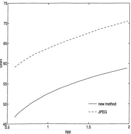
, respectively. The orig­ inal Barbara image and the compressed/decompressed Barbara image with a compression ratio of 6.0 are shown in Figure 3.1. We also coded these images using the Joint Photographic Experts Group (JPEG) compression standard [13]. The comparison of our method with JPEG for the Barbara image and the Lena image are shown in Figure 3.2 and Figure 3.3, respectively. It is seen that JPEG has a better performance than our method at all compression ratios.

Gabor time-frequency atomic decomposition does not have a good perfor­ mance in image coding, although it has a good performance in speech coding. The main reason for this fact is the different characteristics of speech and im­ age signals. A speech signal is an “oscillatory” signal which looks like a typical Gabor atom, hence it can be represented efficiently by Gabor atoms. An imtige signal is non-oscillatory and has different characteristics than a Gabor atom. Therefore, the Gabor decomposition does not give good results for image sig­ nals.

23

Compression Ratio MSDE SNR

0.62 bpp 12.99 13.32 39.48 0.66 bpp 12.20 12.91 40.02 0.71 bpp 11.23 12.40 40.72 0.78 bpp 10.20 11.85 41.51 0.88 bpp 9.05 11.18 42.52 1.03 bpp 7.74 10.36 43.84 1.08 bpp 7.38 10.12 44.25 1.20 bpp 6.67 9.63 45.11 1.33 bpp 6.00 9.14 46.02 1.41 bpp 5.66 8.88 46.52 1.64 bpp 4.88 8.25 47.80 1.78 bpp 4.49 7.90 48.55 2.17 bpp 3.68 7.10 50.42

Table 3.1: The compression results for the Barbara image.

Compression Ratio MSDE SNR

0.59 bpp 13.59 8.96 46.70 0.62 bpp 12.81 8.58 47.45 0.68 bpp 11.79 8.09 48.47 0.76 bpp 10.57 7.56 49.65 0.78 bpp 10.21 7.40 50.02 0.84 bpp 9.51 7.10 50.73 0.92 bpp 8.71 6.75 51.61 0.96 bpp 8.29 6.56 52.11 1.09 bpp 7.34 6.12 53.31 1.17 bpp 6.82 5.88 54.00 1.39 bpp 5.77 5.36 55.61 1.61 bpp 4.96 4.95 57.01 1.97 bpp 4.06 4.45 58.86

24

(b)

25

Figure 3.2: The comparison of the matching pursuit and JPEG algorithms using the Barbara image.

Figure 3.3: The comparison of the matching pursuit and JPEG algorithms using the Lena image.

Chapter 4

Conclusion

In this thesis a new low bit rate speech coding method was developed. The method is based on an adaptive decomposition of speech signals over Gabor time-frequency atoms. This decomposition is elBciently implemented using the matching pursuit algorithm. The new method can code speech signals at a slightly greater bit rate than a standard LPC-10 vocoder, but it produces better quality speech. However, the computational complexity of the new method is large compared to an LPC-10 vocoder. This is mainly due to the calculation of inner products with all atoms in the dictionary.

The new vocoder is a fixed bit rate vocoder. It can also be made a variable bit rate vocoder by making the approximation order of each frame adaptive or using a variable length source coding method such as Pluffman coding. Some of the atoms in the dictionary are selected by the algorithm more frequently than others. The frequency of occurrence of each atom can be found by running the algorithm with long test speeches and then the method can be made variable bit rate using Huffman coding. This can reduce the average bit rate without affecting the speech quality.

Finally, a projection onto convex sets based method was developed to re­ move discontinuities between successive speech frames. The method can re­ move the discontinuities after only a few iterations.

The method for speech coding was also extended to 2-D. For this pur­ pose, 2-D time-frequency atoms were developed. These atoms are used in the matching pursuit algorithm for image coding. Although this method works, its performance is far below a standard JPEG coder. This is because an image signal has different characteristics than a Gabor atom.

References

[1] S. G. Mallat and Z. Zhang, “Matching pursuits with time-frequency dic­ tionaries” , IEEE Transactions on Signal Processing, vol. 41, No. 12, pp. 3397-3415, December 1993.

[2] J. B. Allen and L. R. Rabiner, “A unified approach to short-time Fourier analysis and synthesis” . Proceedings of the IEEE, vol. 65, pp. 1558-1564, 1977.

[3] L. Cohen, “Time-frequency distributions: a review” . Proceedings of the IEEE, vol. 77, No. 7, pp. 941-981, July 1989.

[4] I. Daubechies, Ten Lectures on Wavelets, CBMS-NSF Series in Applied Mathematics, SIAM, 1992.

[5] R. Coifman, Y. Meyer and V. Wickerhauser, “Size properties of wavelet packets” . Wavelets and Their Applications, Mary Beth Ruskai, Ed., Jones and Bartlett Publishers, Boston, pp. 453-470, 1992.

[6] S. Qian and D. Chen, “Signal representation in adaptive normalized Gaus­ sian functions” , submitted to IEEE Transactions on Signal Processing. [7] B. Torresani, “Wavelets associated with representations of the affine Weyl-

Heisenberg group” . Journal of Mathematical Physics, vol. 32, No. 5, pp. 1273-1279, May 1991.

[8] N. S. Jayant, Digital Coding of Waveforms, Prentice-Hall, 1984.

[9] S. Singhal and B. S. Atal, “Amplitude optimization and pitch prediction in multipulse coders” , IEEE Trans, on Acoustics, Speech, and Signal Processing, vol. 37, No. 3, pp. 317-327, March 1989.

[10] V. Cuperman, B. S. Atal and A. Gersho, Advances in Speech Coding, Kluwer Academic Publishers, 1991.

28

[11] Military Agency for Standardization, “NATO standardization agreement, Stanag 4196, parameters and coding characteristics that must be common to assure interoperability of 2400 bps linear predictive encoded digital speech” .

[12] A. Zakhor, “Iterative procedures for reduction of blocking effects in trans­ form image coding” , IEEE Trans, on Circuits and Systems for Video

Technology., vol. 2, No. 1, pp. 91-95, March 1992.

[13] G. K. Wallace, “The JPEG still picture compression standard” . Commu­ nications of the ACM, vol. 34, No. 4, pp. 30-44, April 1991.

[14] N. S. Jayant, “ Coding speech at low bit rates” , IEEE Spectrum, pp. 58-63, August 1986.

[15] L. M. Bregman, “The method of successive projection for finding a com­ mon point of convex sets” , Dokl. Akad. Nauk SSSR, vol. 162, No. 3, 1965. [16] D. C. Youla, “Generalized image restoration by the method of alternating

orthogonal projections” , IEEE Transactions on Circuits and Systems, vol. CAS-25, No. 9, pp. 694-702, September 1978.

[17] A. Papoulis, “A new algorithm in spectral analysis and band-limited extrapolation” , IEEE Transactions on Circuits and Systems, vol. CAS- 22, No. 9, September 1975.