Complex signal recovery from multiple fractional
Fourier-transform intensities
M. Günhan Ertosun, Haluk Atlı, Haldun M. Ozaktas, and Billur Barshan
The problem of recovering a complex signal from the magnitudes of any number of its fractional Fourier transforms at any set of fractional orders is addressed. This problem corresponds to the problem of phase retrieval from the transverse intensity profiles of an optical field at arbitrary locations in an optical system involving arbitrary concatenations of lenses and sections of free space. The dependence of the results on the number of orders, their spread, and the noise is investigated. Generally, increasing the number of orders improves the results, but with diminishing return beyond a certain point. Selecting the measurement planes such that their fractional orders are well separated or spread as much as possible also leads to better results. © 2005 Optical Society of America
OCIS codes: 100.5070, 070.2590, 070.6020.
1. Introduction
The ath-order fractional Fourier domain is a gener-alization of the ordinary space and frequency do-mains. Just as the original function resides in the space domain and its Fourier transform resides in the frequency domain, the ath-order fractional Fourier transform (FRT) of the function1–5resides in the
ath-order fractional Fourier domain.5–10 The ath-order
FRT fa共u兲 of a function f共u兲 is defined for 0 ⬍ |a| ⬍
2 as fa(u)⫽
冕
⫺⬁ ⬁ exp兵⫺i关sgn(␣)兾4 ⫺ ␣兾2兴其ⱍ
sin␣ⱍ
1兾2⫻ exp
关
i共
cot␣u2⫺ 2 csc ␣uu⬘⫹ cot ␣u⬘2
兲兴
f(u⬘)du⬘, (1) where␣ ⫽ a兾2. When a ⫽ 0, we have fa共u兲 ⫽ f共u兲,and when a ⫽ ⫾2, we have fa共u兲 ⫽ f共⫺u兲. When a
⫽ 1, we have f1共u兲 ⫽ F共u兲, the ordinary Fourier
trans-form, and when a⫽ ⫺1, we have f⫺1共u兲 ⫽ F共⫺u兲, the ordinary inverse Fourier transform. The transform is additive in index: the a2th transform of the a1th
transform is equal to the a2⫹ a1th transform and so
forth. The FRT has a fast algorithm.11Further
prop-erties and references are given in Ref. 12.
Phase retrieval from intensity information is a problem of great practical interest and has accord-ingly been extensively studied (for instance, see Refs. 13, 14 and the references therein). In one variation of the problem, the intensity (or magnitude) is known only at one observation plane, such as the Fourier transform plane, and the retrieval process relies on additional assumptions such as finite extent and non-negativity of the original function. In another varia-tion the intensity is known at two planes. These two planes may be the plane of the original object and that of its Fourier transform. Generalization to the case in which the intensity of an object and that of its fractional Fourier transform, or the intensity of any two of its fractional Fourier transforms, is known has been addressed in.15–20
Here we consider the even more general case in which the intensity (or magnitude) of the signal is known at any number of arbitrary fractional Fourier domains (or, in other words, we know the magnitude of the FRT of the function at an arbitrary set of or-ders). It has been shown that the propagation of op-tical waves can be characterized by the FRT, with the transverse amplitude of light going through frac-tional Fourier transforms of increasing order as light propagates along the optical axis. Mathematically,
M. G. Ertosun ([email protected]) is with the Department of Electrical Engineering, Stanford University, Stanford, California 94305. H. Altı ([email protected]) is with Vestel Communi-cation R&D Group, Aegean Free Zone, Izmir 35410, Turkey. H. M. Ozaktas and B. Barshan are with the Department of Electrical Engineering, Bilkent University, TR-06800 Bilkent, Ankara, Tur-key.
Received 15 September 2004; revised manuscript received 25 February 2005; accepted 1 March 2005.
0003-6935/05/234902-07$15.00/0 © 2005 Optical Society of America
this result is expressed as a relation between the FRT and the Fresnel integral, with the transform order’s being related to the distance of propagation.12,21
Therefore the problem of recovering a complex signal fully from its FRT magnitudes at multiple orders can be used to solve the problem of recovering a complex field from multiple transverse intensity profiles at arbitrary locations along the optical axis. In other words, if we cannot measure the phase at a certain plane, we can compensate by measuring the intensity at other planes.
Furthermore, optical systems involving arbitrary concatenations of thin lenses and sections of free space in the Fresnel approximation can also be mod-eled in terms of the FRT.12,21 Such systems are
known as quadratic-phase systems, ABCD optical systems, among other names. This means that the transverse amplitude of light at any arbitrary plane of such a system can be related to the transverse amplitude at any other plane through a FRT relation. Therefore the problem addressed here can also be used for recovering the complex field from multiple transverse intensity profiles at arbitrary locations in such a system. In other words, the problem we deal with here does not require that the several planes be related through a Fourier transform or free-space propagation and is more general.
A fundamental algorithm used to recover phase from the magnitudes of a function and its Fourier transform is known as the Gerchberg–Saxton (GS) iterative algorithm.22Many refinements of this basic
algorithm have been considered; for instance, see Refs. 13, 14, 23, and 24. A variation of the algorithm to deal with arbitrary general linear systems (not necessarily unitary like the Fourier or fractional Fou-rier transforms) has also been presented.25–27In this
paper we consider the generalization of the two-intensity phase retrieval problem to the multiple-intensity phase retrieval problem as well as the multiple-domain GS algorithm in their purest forms so as to reveal the effects of working with multiple fractional domains as transparently as possible; and we refrain from carrying over extensions or refine-ments proposed for the basic GS algorithm. We also do not make use of any additional prior knowledge (such as nonnegativity and so forth) other than the magnitudes.
The use of the GS algorithm in conjunction with FRTs has been reported in a number of earlier papers,15,17–20,28 –30 which are comparatively
dis-cussed in Ref. 15. All of these studies deal with two fractional domains. [A number of studies deal with the retrieval of phase from FRT magnitudes at all orders.31–33Such tomographic methods are inefficient
when they are applied to fully coherent or determin-istic fields that require a large number of measure-ments (see Ref. 12, pp. 378 –380 and Refs. 34 –36). A number of other studies deal with the problem of recovering phase from two fractional domains whose orders are close.37–39]
The problem of phase retrieval from FRT magni-tudes is related to the problem of phase retrieval from
Fresnel transform magnitudes.40 – 47 However, the
problem of retrieval from more than two Fresnel transforms does not seem to have received anywhere near the attention received by the two-intensity problem. Nevertheless, it has been demonstrated in various contexts that phase information can be recov-ered from multiple Fresnel intensities.48 –52The
prob-lem of recovery from multiple-intensity observations related through general linear transformations is dis-cussed in Ref. 53.
Formulating the problem in terms of FRTs is con-sistent with the description of optical propagation through ABCD optical systems as continuous FRT and evolution of the light field through increasing FRT orders. In addition to being mathematically purer, FRT has several advantages. FRT satisfies a more complete and elegant set of basic properties. The concept of fractional Fourier domains7,8allows us
to more transparently understand the working of the GS algorithm as the signal is iterated through do-mains of different orders, whereas a corresponding concept of Fresnel domains is not so well established. The FRT formulation facilitates a systematic and general study of the variation of key parameters and the derivation of fairly general conclusions. Since FRT corresponds to pure rotation in the space– frequency plane (rather than to shearing as in the Fresnel transform), it is geometrically and numeri-cally better behaved.
2. Results
We assume that the magnitude |fan共u兲| or
inten-sity |fan共u兲|
2of the a
nth fractional Fourier transform
of a complex function f共u兲 is known at M orders a1
⬍ a2⬍ . . . ⬍ aM. Our aim is to recover the unknown
function f共u兲. Since the fractional order a is periodic with periodicity 4 and since f⫾2共u兲 ⫽ f共⫺u兲, we can restrict the values of anto the interval关0, 2兲 without
loss of generality.
The GS algorithm employed can be summarized as follows. We begin by initializing the unknown phase function of fa1共u兲 to some initial value, such as zero
or a constant. Then we take the a2⫺ a1th-order FRT
of fa1共u兲. We leave the calculated phase intact but
replace the magnitude with the known magnitude of
fa2共u兲. Then we take the a3⫺ a2th-order FRT of this
function and again leave the calculated phase intact and replace the magnitude with the known magni-tude of fa3共u兲. We continue in this manner until we
reach faM共u兲, whose a1⫺ aMth-order FRT we take to
return to the domain we started with. The iteration cycle is then repeated. Since functions differing by a constant phase would have the same fractional Fou-rier magnitudes, recovery is possible up to a constant phase factor. In plotting the final recovery errors in the following examples, we have eliminated this con-stant phase.
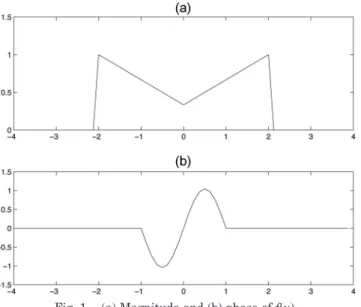
The example signal employed is shown in Fig. 1. A large percentage of the signal energy is contained in a space–frequency region of radius 4 so that in all domains we restrict our attention to the interval
u僆 关⫺4, 4兴. The Nyquist theorem implies a sampling
interval in each domain that is equal to the inverse of the extent of the signal in the orthogonal domain, which leads to a sampling interval of 1兾8 and a space– bandwidth product of 64 in all domains. Ei-ther the discrete FRT matrix defined in Ref. 54 or the algorithm described in Ref. 11 can be employed to compute the FRTs to a good approximation; the former approach was employed here. The GS algo-rithm uses the magnitudes of the FRTs of the func-tion displayed as its input. The phase is initialized to zero. The final error between the iterate and the orig-inal phase function共u兲 is defined as
冋
共1兾8兲冕
⫺4 4ⱍ
k(u)⫺ (u)ⱍ
2du册
1兾2 . (2)Although this equation is used as a measure of the final error for the purpose of this paper, we note that, in practice,共u兲 is not known beforehand. The issue of when to stop the iterations is similar to that encoun-tered in other studies that dealt with iterative phase retrieval and is therefore not a focus of this paper.
As a generic example, we assume that the intensi-ties happen to be known at the orders 0.0, 0.3, 0.7, 0.9, and 1.9. In this example by employing the out-lined method, the final error drops below 0.001 within 10 iterations.
Although this method is generally valid for an ar-bitrary set of an, as illustrated by the above example,
for purposes of illustration and determining the effect of the number of orders on the results systematically, we discuss the case in which the orders are evenly spaced. Two variations are considered. In variation A the M orders are chosen as 0.0, 0.2, 0.4, . . . , 0.2 ⫻ 共M ⫺ 1兲. In other words, regardless of the number of orders, the spacing remains the same. In variation
B the M orders are spread evenly over the range关0, 2兲 as 0, 2兾M, 4兾M, . . . , 2共M ⫺ 1兲兾M. Here, regardless of their number, the orders span the whole range of a. We consider values of M ranging from 2 to 8.
Figure 2 shows the final error between the iterate and the original phase function 共u兲. In most cases the error decreases to small values within ⬃100 it-erations. For alternative A, we observe that conver-gence is faster when M is larger and worse when M is smaller. This is understandable: Larger values of M mean that a greater amount of information is avail-able for and applied to the solution of the problem so that we reach smaller errors more quickly. This may not be a fair comparison since the computation time for an iteration is actually proportional to M. How-ever, from the figure we see that this conclusion tends to remain true even when the error is plotted as a function of computation time. Although not as clear cut, similar conclusions can be made for alternative B, with the exception that much smaller errors are obtained for M⫽ 2 (smaller than 0.001). The reason for this exception is that for small values of M, the disadvantage of having fewer orders is offset by the advantage of having the spacing between the orders equal to unity. (It was shown in Ref. 15 that conver-gence was faster and smaller errors were obtained when the spacing between the orders is close to unity.) It is important to note that this exception is not fundamental but rather a result of the way we constructed our uniformly spaced illustrative exam-ples. It may nevertheless be concluded that a greater separation between the orders has a positive effect on the results, as evidenced by the fact that the errors for variation B are generally smaller than those for variation A, for the same M. When the orders are farther apart, they represent more independent pieces of information.
We now consider the effects of adding various amounts of zero-mean white Gaussian noise to the observed FRT magnitudes. The signal-to-noise ratio (SNR) is defined as SNR⫽
冕
⫺4 4ⱍ
f(u)ⱍ
2du冕
⫺44 2du , (3)where2 is the variance of the zero-mean Gaussian
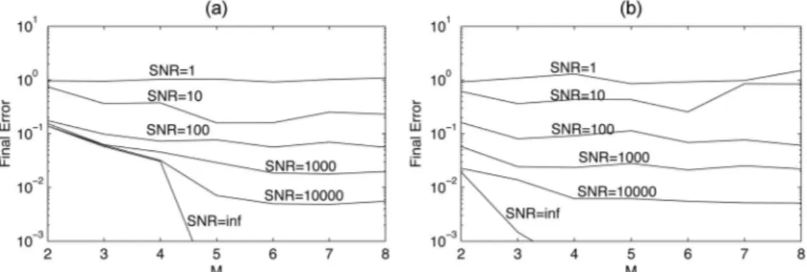
random variable characterizing each sample of the noise process. Figure 3 gives the final errors between the 10th and 100th iterates and the original phase function for different amounts of added noise for vari-ation A. As expected, the final error increases as the noise increases for any given order. When SNR⫽ 1, all the final errors are very large and do not depend much on the order. As the SNR increases, we begin to observe a decrease in the final error with increasing
M. This decrease with order is most pronounced for
the largest SNR values. Also, with increasing number of iterations, the errors for smaller values of M be-come closer to those for larger values of M, so that the decrease with M becomes less pronounced.
Knowing the magnitude at a greater number of orders reduces the negative effects of noise through increased redundancy and noise-averaging effects. Since the noise added to the measurements at the M different orders are independent, we might very crudely expect a共M兾2兲1兾2factor of effective SNR im-provement with respect to the case in which only two intensites are known. (For example, the case M⫽ 8 with SNR ⫽ 1000 would crudely correspond to the
case M ⫽ 2 with SNR ⫽ 2000.) Since this crude argument indicates that the effect of increasing M in combating the effects of noise is modest and much less than the improvements observed with increasing
M, we conclude that the reduction of the effects of
noise is not the major contributor to the reduction in error obtained with increasing M. Since the error quickly falls to very small values when there is no noise for even moderate values of M, the noise rather than the structural features of the problem can be said to be responsible for the final error in the pres-ence of noise.
We must also note that the errors in Fig. 3 were computed according to the modified error formula
Fig. 2. Final recovery error. The right-hand plots contain the same data as the left-hand plots, with the horizontal axis scaled to correspond to the actual time of computation: Time⫽ M ⫻ Number of iterations. (a), (b), variation A; (c), (d), variation B.
冋
共1兾4兲冕
⫺2 2ⱍ
k(u)⫺ (u)ⱍ
2du册
1兾2 . (4)to exclude the regions where the magnitude of the original function is identically zero. When the mag-nitude is identically zero, we cannot expect to retrieve the phase, which is indeterminate. Owing to this in-determinacy, the algorithm is very sensitive to even the smallest amount of noise and results in random-like and highly erroneous results outside the interval 关⫺2, 2兴. Including these randomlike results in the final error leads to meaningless results. Of course, in practice we may not know that the actual noiseless magnitude was exactly zero outside this interval, and formal or informal application of additional con-straints or knowledge would be needed to decide that the randomlike results obtained outside关⫺2, 2兴 con-stitute an amplification of noise and not a reconstruc-tion of the phase in that region.
Although we expect most of the results of this pa-per to also hold true for the two-dimensional case, it would be necessary to conduct additional simulations to make definitive conclusions.
As a final remark before leaving this section, we note that it has been shown that if the Fourier trans-form intensity can be oversampled at a rate suffi-ciently higher than the Nyquist rate, then the phase can be retrieved by using an iterative algorithm.16,23
It would be interesting to inquire whether the same would be true for FRT intensities and what the im-plications of this would be to two- and multiple-intensity problems.
3. Discussion and Conclusions
In this paper we have considered the problem of re-covering complex signals from multiple magnitude (or intensity) measurements at an arbitrary set of FRT orders. While showing that the method works for any set of orders, we have also constructed two variations of systematically chosen orders to investi-gate the dependence of the results on the number of orders, their spread, and the noise.
This problem corresponds to the problem of recover-ing the complex field from multiple transverse inten-sity profiles at arbitrary locations in an optical system that involves arbitrary concatenations of lenses and sections of free space and is not limited to the case in which the several planes are related through Fourier transforms or free-space propagation.
We have observed that knowing the magnitude (or intensity) of the FRT of a function at more than 2 orders has a positive effect on the results by decreas-ing the final error. Generally, increasdecreas-ing the number of known orders improves the results; however, be-yond a certain number of orders, further increases have diminishing returns. This is understandable since the information that comes with additional or-ders becomes increasingly redundant with increasing
M. Such redundant information is useful up to a
cer-tain point but not after that. In fact, since increasing the number of orders M also increases the
computa-tional time per iteration, increasing M too much may result in a slower reduction of the error as a function of real time. It is not possible to be very specific re-garding the precise value of M after which improve-ments saturate, but in general it seems that values of
M beyond the order of 10 are not useful. This also
confirms that tomographic methods that employ a large number of orders are not efficient.
In terms of information, the complex function we wish to recover is equivalent to two independent real functions. Two intensity measurements at different fractional orders共M ⫽ 2兲 also correspond to two real functions. However, since the problem is not linear or convex, these two measurements do not necessarily lead to a unique solution, or at least they do not ensure an efficient convergence to such a solution. One may be confronted with stagnation of the algo-rithm or slow progress in a “tunnel” (see Ref. 13, p. 304). Unlike in two dimensions, where uniqueness is usually ensured, in one dimension the solution of the conventional two-intensity phase retrieval problem is not unique.55 Increasing M beyond 2 orders helps
overcome these difficulties.
The effect of noise is to equalize the dependence on the number of orders M. When the noise is small, the final errors depend more strongly on M, with smaller
M tending to result in greater error. As the noise is
increased, the final errors obtained with different M become closer, and for large noise values correspond-ing to unity SNR, the final errors are roughly com-parable for all M. Generally speaking, for a given M, the final error decreases with decreasing noise as expected, with the amount of decrease greater for higher M. Likewise, for a given SNR, final error de-creases with increasing M, with the decrease greater for higher values of SNR. We also observed that the benefits of using larger versus smaller values of M were especially pronounced for the case of large SNR and small iteration numbers, an observation that might be especially useful when the need to obtain solutions in real time severely limits the number of feasible iterations.
The final error has two main constituents, a noise-independent one and a noise-dependent one. The noise-independent contribution is pronounced when M is small and is a result of the nonlinear, nonconvex nature of the problem. This contribution quickly de-creases as M inde-creases. On the other hand, the noise-dependent contribution does not depend strongly on M. We observed that for a given number of orders, spreading them over the whole range of a resulted in smaller errors when compared with spreading them over a smaller range. It may be concluded that greater separation between orders has a positive ef-fect on the results. When the orders are farther apart from one another, they represent more independent pieces of information. When the orders are clustered or close to one another, the problem becomes more ill posed. Knowledge of the magnitudes clustered or close to one another is less desirable, whereas knowl-edge of the magnitudes at orders that are well sepa-rated or spread over the range of a is more desirable.
It follows from the discussion in the previous para-graph that if multiple-intensity measurements are to be made in an optical system and if it is desirable to retrieve the phase from these measurements, it would be best to select the measurement planes such that they correspond to FRTs whose orders are well separated or spread over the range of a. This conclu-sion, which follows immediately from our FRT-based formulation, might have been less evident in a Fresnel-transform-based approach. The well-known relation between quadratic-phase optical systems and FRT enables one to easily find the locations along the optical axis that correspond to given fractional orders. Therefore, given any physical or mechanical constraints of the system, the orders can be chosen in the most suitable manner.
H. M. Ozaktas acknowledges partial support of the Turkish Academy of Sciences.
References
1. D. Mendlovic and H. M. Ozaktas, “Fractional Fourier trans-forms and their optical implementation: I,” J. Opt. Soc. Am. A
10, 1875–1881 (1993).
2. H. M. Ozaktas and D. Mendlovic, “Fractional Fourier trans-forms and their optical implementation: II,” J. Opt. Soc. Am. A
10, 2522–2531 (1993).
3. A. W. Lohmann, “Image rotation, Wigner rotation, and the fractional order Fourier transform,” J. Opt. Soc. Am. A 10, 2181–2186 (1993).
4. L. B. Almeida, “The fractional Fourier transform and time-frequency representations,” IEEE Trans. Signal Process. 42, 3084 –3091 (1994).
5. H. M. Ozaktas, B. Barshan, D. Mendlovic, and L. Onural, “Convolution, filtering, and multiplexing in fractional Fourier domains and their relation to chirp and wavelet transforms,” J. Opt. Soc. Am. A 11, 547–559 (1994).
6. H. M. Ozaktas, B. Barshan, and D. Mendlovic, “Convolution and filtering in fractional Fourier domains,” Opt. Rev. 1, 15–16 (1994).
7. O. Aytür and H. M. Ozaktas, “Non-orthogonal domains in phase space of quantum optics and their relation to fractional Fourier transforms,” Opt. Commun. 120, 166 –170 (1995). 8. H. M. Ozaktas and O. Aytür, “Fractional Fourier domains,”
Signal Process. 46, 119 –124 (1995).
9. M. A. Kutay, H. Özaktas¸, H. M. Ozaktas, and O. Arıkan, “The fractional Fourier domain decomposition,” Signal Process. 77, 105–109 (1999).
10. ˙I. S¸ . Yetik, M. A. Kutay, H. Özaktas¸, and H. M. Ozaktas, “Continuous and discrete fractional Fourier domain decompo-sition,” in Proceedings of the 2000 IEEE International
Conference on Acoustics, Speech, and Signal Processing,
(In-stitute of Electrical and Electronics Engineers, 2000), pp. I:93– 96.
11. H. M. Ozaktas, O. Arıkan, M. A. Kutay, and G. Bozdag˘ı, “Dig-ital computation of the fractional Fourier transform,” IEEE Trans. Signal Process. 44, 2141–2150 (1996).
12. H. M. Ozaktas, Z. Zalevsky, and M. A. Kutay, The Fractional
Fourier Transform with Applications in Optics and Signal Processing (Wiley, 2001).
13. H. Stark, ed., Image Recovery: Theory and Application (Aca-demic, 1987).
14. H. H. Bauschke, P. L. Combettes, and D. R. Luke, “Phase retrieval, error reduction algorithm, and Fienup variants: a view from convex optimization,” J. Opt. Soc. Am. A 19, 1334 – 1345 (2002).
15. M. G. Ertosun, H. Atlı, H. M. Ozaktas, and B. Barshan, “Com-plex signal recovery from two fractional Fourier transform intensities: order and noise dependence,” Opt. Commun. 244, 61–70 (2005).
16. J. Miao, D. Sayre, and H. N. Chapman, “Phase retrieval from the magnitude of the Fourier transforms of nonperiodic ob-jects,” J. Opt. Soc. Am. A 15, 1662–1669 (1998).
17. B. Dong, Y. Zhang, B. Gu, and G. Yang, “Numerical investi-gation of phase retrieval in a fractional Fourier transform,” J. Opt. Soc. Am. A 14, 2709 –2714 (1997).
18. W.-X. Cong, N.-X. Chen, and B.-Y. Gu, “Recursive algorithm for phase retrieval in the fractional Fourier transform do-main,” Appl. Opt. 37, 6906 – 6910 (1998).
19. W.-X. Cong, N.-X. Chen, and B.-Y. Gu, “A new method for phase retrieval in the optical system,” Chin. Phys. Lett. 15, 24 –26 (1998).
20. W.-X. Cong, N.-X. Chen, and B.-Y. Gu, “A recursive method for phase retrieval in Fourier transform domain,” Chin. Sci. Bull.
43, 40 – 44 (1998).
21. H. M. Ozaktas and D. Mendlovic, “Fractional Fourier optics,” J. Opt. Soc. Am. A 12, 743–751 (1995).
22. R. W. Gerchberg and W. O. Saxton, “A practical algorithm for the determination of phase from image and diffraction plane pictures,” Optik (Stuttgart) 35, 237–246 (1972).
23. J. R. Fienup, “Phase retrieval algorithms: a comparison,” Appl. Opt. 21, 2758 –2769 (1982).
24. J. C. Dainty and J. R. Fienup, “Phase retrieval and image reconstruction for astronomy,” in Image Recovery: Theory and
Application, H. Stark, ed. (Academic, 1987), pp. 231–275.
25. G. Yang and B. Gu, “On the amplitude-phase retrieval problem in the optical system,” Acta Phys. Sin. 30, 410 – 413 (1981). 26. B. Gu and G. Yang, “On the phase retrieval problem in optical
and electronic microscopy,” Acta Opt. Sin. 1, 517–522 (1981). 27. G. Yang, B. Dong, B. Gu, J. Zhuang, and O. K. Ersoy, “Gerchberg–Saxton and Yang–Gu algorithms for phase re-trieval in a nonunitary transform system: a comparison,” Appl. Opt. 33, 209 –218 (1994).
28. Z. Zalevsky, D. Mendlovic, and R. G. Dorsch, “Gerchberg– Saxton algorithm applied in the fractional Fourier or the Fresnel domain,” Opt. Lett. 21, 842– 844 (1996).
29. Y. Zhang, B. Dong, B. Gu, and G. Yang, “Beam shaping in the fractional Fourier transform domain,” J. Opt. Soc. Am. A 15, 1114 –1120 (1998).
30. B. Hennelly and J. T. Sheridan, “Fractional Fourier transform-based image encryption: phase retrieval algorithm,” Opt. Com-mun. 226, 61– 80 (2003).
31. M. G. Raymer, M. Beck, and D. F. McAlister, “Complex wave-field reconstruction using phase-space tomography,” Phys. Rev. Lett. 72, 1137–1140 (1994).
32. D. F. McAlister, M. Beck, L. Clarke, A. Mayer, and M. G. Raymer, “Optical phase retrieval by phase-space tomography and fractional-order Fourier transforms,” Opt. Lett. 20, 1181– 1183 (1995).
33. X. Liu and K.-H. Brenner, “Reconstruction of two-dimensional complex amplitudes from intensity measurements,” Opt. Com-mun. 225, 19 –30 (2003).
34. D. Dragoman, “Redundancy of phase-space distribution func-tions in complex field recovery problems,” Appl. Opt. 42, 1932– 1937 (2003).
35. M. Testorf, “Comment on ‘Redundancy of phase-space distri-bution functions in complex field recovery problems’,” Appl. Opt. 44, 55–57 (2005).
36. D. Dragoman, “Reply to comment on ‘Redundancy of phase-space distribution functions in complex field recovery prob-lems’,” Appl. Opt. 44, 58 –59 (2005).
37. T. Alieva and M. J. Bastiaans, “On fractional Fourier trans-form moments,” IEEE Signal Process. Lett. 7, 321–323 (2000).
38. T. Alieva, M. J. Bastiaans, and L. Stankovic, “Signal recon-struction from two close fractional Fourier power spectra,” IEEE Trans. Signal Process. 51, 112–123 (2003).
39. M. Bastiaans and K. Wolf, “Phase reconstruction from inten-sity measurements in linear systems,” J. Opt. Soc. Am. A 20, 1046 –1049 (2003).
40. R. Rolleston and N. George, “Image reconstruction from partial Fresnel zone information,” Appl. Opt. 25, 178 –183 (1986). 41. R. Rolleston and N. George, “Stationary phase approximations
in Fresnel-zone magnitude-only reconstructions,” J. Opt. Soc. Am. A 4, 148 –153 (1987).
42. D. L. Misell, “A method for the solution of the phase problem in electron microscopy,” J. Phys. D 6, L6 –L9 (1973). 43. D. L. Misell, “An examination of an iterative method for the
solution of the phase problem in optics and electron optics: I. Test calculations,” J. Phys. D 6, 2200 –2216 (1973).
44. D. L. Misell, “An examination of an iterative method for the solution of the phase problem in optics and electron optics: II. Sources of error,” J. Phys. D 6, 2217–2224 (1973).
45. T. E. Gureyev, A. Pogany, D. M. Paganin, and S. W. Wilkins, “Linear algorithms for phase retrieval in the Fresnel region,” Opt. Commun. 231, 53–70 (2004).
46. T. E. Gureyev, “Composite techniques for phase retrieval in the Fresnel region,” Opt. Commun. 220, 49 –58 (2003). 47. W.-X. Cong, N.-X. Chen, and B.-Y. Gu, “Phase retrieval in the
Fresnel transform system: a recursive algorithm,” J. Opt. Soc. Am. A 16, 1827–1830 (1999).
48. W. Coene, G. Janssen, M. Op de Beeck, and D. Van Dyck, “Phase retrieval through focus variation for ultra-resolution in field-emission transmission electron microscopy,” Phys. Rev. Lett. 69, 3743–3746 (1992).
49. K. A. Nugent, T. E. Gureyev, D. Cookson, D. Paganin, and Z. Barnea, “Quantitative phase imaging using hard x rays,” Phys. Rev. Lett. 77, 2961–2964 (1996).
50. L. J. Allen, W. McBride, and M. P. Oxley, “Exit wave recon-struction using soft x-rays,” Opt. Commun. 233, 77– 82 (2004). 51. L. J. Allen and M. P. Oxley, “Phase retrieval from series of images obtained by defocus variation,” Opt. Commun. 199, 65–75 (2001).
52. L. J. Allen, H. M. L. Faulkner, K. A. Nugent, M. P. Oxley, and D. Paganin, “Phase retrieval from images in the presence of first-order vortices,” Phys. Rev E 63, 037602-1– 037602-4 (2001). 53. V. Yu. Ivanov, V. P. Sivokon, and M. A. Vorontsov, “Phase retrieval from a set of intensity measurements: theory and experiment,” J. Opt. Soc. Am. A 9, 1515–1524 (1992). 54. C. Candan, M. Alper Kutay, and H. M. Ozaktas, “The discrete
fractional Fourier transform,” IEEE Trans. Signal Process. 48, 1329 –1337 (2000).
55. R. P. Millane, “Phase retrieval in crystallography and optics,” J. Opt. Soc. Am. A 7, 394 – 411 (1990).