DEVELOPMENT OF A SUPERVISORY
CONTROLLER FOR ENERGY
MANAGEMENT PROBLEMS
a thesis
submitted to the department of mechanical engineering and the graduate school of engineering and science
of bilkent university
in partial fulfillment of the requirements for the degree of
master of science
By
Emre Akg¨
un
I certify that I have read this thesis and that in my opinion it is fully adequate, in scope and in quality, as a thesis for the degree of Master of Science.
Asst. Prof. Dr. Melih C¸ akmakcı(Advisor)
I certify that I have read this thesis and that in my opinion it is fully adequate, in scope and in quality, as a thesis for the degree of Master of Science.
Asst. Prof. Dr. Sinan Filiz
I certify that I have read this thesis and that in my opinion it is fully adequate, in scope and in quality, as a thesis for the degree of Master of Science.
Asst. Prof. Dr. Yi˘git Karpat
Approved for the Graduate School of Engineering and Science:
Prof. Dr. Levent Onural Director of the Graduate School
ABSTRACT
DEVELOPMENT OF A SUPERVISORY CONTROLLER
FOR ENERGY MANAGEMENT PROBLEMS
Emre Akg¨un
M.S. in Mechanical Engineering Supervisor: Asst. Prof. Dr. Melih C¸ akmakcı
July, 2011
Multi energy source systems, like hybrid electric vehicles in automotive industry, started to attract attention as a remedy for the greenhouse gas emission prob-lem. Although their environmental performances are better than conventional technologies such as the case of gasoline vehicles versus hybrid electric vehicles in automotive industry, their operational management can be challenging due to their increased complexity. One of these challenges is the operational manage-ment of the energy flow among these multiple sources and sinks which in this context referred as the energy management problem.
In this thesis, a supervisory controller is developed to operate at a residential environment with multiple energy sources. First, dynamic optimization tech-niques are applied to the available mathematical models of the multi-energy sources to create a non-causal optimal controller. Then, a set of implementable rules are extracted by analyzing the optimal trajectories resulted from the dy-namic optimization to create a causal supervisory controller.
Several simulations are conducted with Matlab/Simulink to validate the de-veloped controller. The supervisory controller achieves not only a daily cost reduction between 6-7.5% compared to conventional energy infrastructure used in residential areas but also performs 2% better than heuristic control techniques available in the literature. Another simulation study is conducted, with differ-ent demand cycles, for verification of the controller. Although its performance reduces as expected, it still performs 1% better than heuristic control strategies. In the final part of this thesis, the formulation used in the residential problem which was originally adopted from an example in automotive industry, is general-ized so that it can be used in all types of energy management problems. Finally, for exemplary purposes, a formulation for energy management problem in mobile
iv
devices is created by using the developed generic formulation.
¨
OZET
ENERJ˙I Y ¨
ONET˙IM˙I PROBLEMLER˙I ˙IC
¸ ˙IN Y ¨
ONET˙IC˙I
T˙IPTE KONTROLC ¨
U TASARIMI
Emre Akg¨un
Makine M¨uhendisli˘gi, Y¨uksek Lisans Tez Y¨oneticisi: Asst. Prof. Dr. Melih C¸ akmakcı
Temmuz, 2011
G¨un¨um¨uzde, birden fazla enerji kayna˘gına sahip olan sistemlerin, ¨orne˘gin hib-rit otomobiller, pop¨uleritesinin arttı˘gı g¨ozlemlenmektedir. Bu durumun altında yatan ba¸slıca sebep ise ¸cok kaynaklı enerji sistemlerinin ¸cevresel y¨onden ¸su anda kullandı˘gımız tek kayna˘ga ba˘glı enerji sistemlerinden, benzinli arabalar gibi, daha ba¸sarılı bir performans g¨ostermesidir. ¨Ote yandan bu tip birden fazla kaynaklı sistemler sundukları yeni operasyon modları sayesinde mevcut sistemlerden daha verimli ¸calı¸sma potansiyeline sahiptirler. Fakat do˘gru operasyon modunu ve buna ili¸skin g¨u¸c seviyelerini belirlemek sorun te¸skil etmektedir. Bu problem enerji y¨onetimi problemi olarak adlandırılmı¸stır.
Bu tezde ¸coklu kayna˘ga sahip bir yerle¸sim alanının enerji y¨onetimi prob-lemini ¸c¨ozmek i¸cin y¨onetici tipte bir kontrolc¨u tasarlanmı¸stır. Bu do˘grultuda ¨
oncelikle literat¨urde varolan matematiksel modellerden yararlanılarak sistem i¸cin bir dinamik optimizasyon form¨ulasyonu olu¸sturulmu¸stur. Daha sonra dinamik optimizasyon ¸cıktılarından yararlanılarak ger¸cek hayatta uygulanabilecek kural-lar ¸cıkartılmı¸s ve kontrolc¨u olu¸sturulmu¸stur.
Matlab/Simulink ortamında yapılan sim¨ulasyonlar sonucu, tasarlanan kon-trolc¨un¨un literat¨urde varolan sezgisel kontrolc¨ulerden, se¸cilen t¨um performans parametrelerinde, g¨unl¨uk olarak yakla¸sık %1-2 daha iyi performans g¨osterdi˘gi saptanmı¸stır.
Bu tez, daha ¨once otomotiv sekt¨or¨unde uygulanmı¸s bir ¸c¨oz¨umden yola ¸cıkılarak ev ortamı i¸cin yaratılan kontrolc¨un¨un genelle¸stirilmesi ile tamam-lanmı¸stır. Bu genel form¨ulasyon kullanılarak farklı alanlardaki enerji y¨onetimi problemleri ¸c¨oz¨ulebilmektedir. Yaratılan genel formun kullanımını g¨ostermek amacıyla amacıyla mobil cihazlarda enerji y¨onetimi yapmak i¸cin bir form¨ulizasyon
vi
g¨osterilmi¸stir.
Anahtar s¨ozc¨ukler : Enerji Y¨onetimi, Dinamik Programlama, Y¨onetici tipte kon-trolc¨u.
Acknowledgement
I would like to express my gratitude to my advisor, Dr. Melih C¸ akmakcı for his incredible patience, support and valuable guidance throughout this work.
I also would like to thank Dr. Sinan Filiz and Prof. Adnan Akay for their classes and vision they provided during my master’s studies, which was an in-valuable experience and improved me a lot as an engineer.
Finally, thanks to my family for their great support and encouragement.
Contents
1 Introduction 1
1.1 Energy Management Problem (EMP) . . . 1
1.2 Background and Literature Review . . . 4
1.2.1 EMP for Automotive Industry . . . 4
1.2.2 Residential EMP . . . 6
1.2.3 EMP for Portable Devices . . . 9
1.3 Motivation . . . 11
1.3.1 Contributions . . . 11
2 Residential Energy Management Problem 12 2.1 System Definition and Possible Frameworks . . . 12
2.2 Mathematical Model . . . 15
2.2.1 Converter Devices Used in the Residential System . . . 17
2.2.2 Energy Demand Cycles . . . 26
2.3 Optimal Trajectory Generation . . . 28
CONTENTS ix
2.4 Real-Time Supervisory Control . . . 35
2.4.1 Creating Rules . . . 36
2.4.2 Charge-Sustaining Strategy . . . 40
2.4.3 Rule Sensitivity . . . 42
2.4.4 Comparison with Optimal Trajectories . . . 43
2.5 Simulations . . . 46
2.5.1 Performance Assessment Parameters . . . 47
2.5.2 Simulation I: Validation of the developed supervisory con-troller . . . 48
2.5.3 Simulation II: Verification of the developed supervisory controller . . . 50
3 Generic Formulation for EMP 53 3.1 Definitions and framework . . . 54
3.2 System optimization . . . 57
3.3 Developing Generic Baseline Control Strategy . . . 61
3.4 Example for Generic Formulation: HEVs . . . 65
3.5 Example for Generic Formulation: Mobile Devices . . . 73
4 Conclusions and Future Work 78 4.1 Future Work . . . 79
CONTENTS x
A Parameterization Study 87
B MATLAB Code 89
List of Figures
1.1 Multi-source Multi-Sink System . . . 2
1.2 Micro Generation System . . . 7
2.1 Graphical Representation of the System Worked . . . 14
2.2 HEV Backward Facing Model . . . 16
2.3 Backward Facing Model of the Proposed System . . . 17
2.4 Backward facing, quasi-static representation of mCHP device . . . 18
2.5 HPR vs. Fraction Electrical Load (X) . . . 20
2.6 SFC vs. Fraction Electrical Load (X) . . . 20
2.7 Electrical Efficiency vs. Fraction Electrical Load (X) . . . 21
2.8 SOC vs. Battery Internal Resistance . . . 23
2.9 Backward facing, quasi-static representation of boiler . . . 24
2.10 Electricity demand profile throughout a day [31] . . . 26
2.11 DHW demand profile throughout a day [31] . . . 27
2.12 SPH demand profile throughout a day [9] . . . 28
LIST OF FIGURES xii
2.13 DP Procedure . . . 29
2.14 Power Split Method . . . 30
2.15 Optimal State Trajectory . . . 34
2.16 Optimal Usage of Devices Throughout the Day . . . 35
2.17 Operation modes for residential system . . . 37
2.18 Battery Operation with respect to Electricity Demand . . . 38
2.19 Power Split for Battery Operation . . . 38
2.20 Power Split between Electricity Grid and mCHP . . . 39
2.21 Control Strategy . . . 41
2.22 Average Daily Electricity Consumption in Winter . . . 42
2.23 Average Daily DHW Consumption in Winter . . . 43
2.24 DP Results Compared to Real-Time Controller . . . 44
2.25 Daily electricity demand of a typical house . . . 50
2.26 Comparison of Optimal Trajectory with new demand cycles . . . 51
3.1 Contour Map . . . 62
3.2 Control Strategy . . . 64
3.3 Parallel HEV Layout from [35] . . . 65
3.4 Example optimal SOC trajectory . . . 70
3.5 Example sparse operation points for HEV . . . 71
LIST OF FIGURES xiii
3.7 Control Strategy for HEV . . . 72
3.8 Control Strategy for Mobile Devices . . . 77
A.1 Convergence Analysis Conducted on State Grid . . . 87
A.2 Convergence Analysis Conducted on Control Inputs Grid . . . 88
List of Tables
2.1 Possible Household Devices . . . 13
2.2 Parameters for mCHP . . . 22
2.3 Parameters for battery . . . 24
2.4 Parameters for battery . . . 25
2.5 Usage Frequency of Multi-Sources in a day (24h) . . . 48
2.6 Cost and Primary Energy Reduction (24h) . . . 49
2.7 Cost and Primary Energy Reduction (24h) . . . 52
3.1 Case Specific Examples . . . 55
3.2 Vectors for HEV . . . 66
3.3 Operation Modes for HEV . . . 66
3.4 Cost Function Construction . . . 67
3.5 State Determination . . . 68
3.6 Generic Energy Management Problem . . . 69
3.7 Vectors for Mobile Devices . . . 75
LIST OF TABLES xv
3.8 Cost Function Construction for Mobile Devices . . . 75 3.9 Mobile Energy Management Problem . . . 76
Chapter 1
Introduction
In the first section of this chapter, the problem worked on in this thesis, energy management, is explained. In the subsequent sections, three industries that are facing this problem is introduced. Finally, this chapter concluded with motivation and contributions of this thesis.
1.1
Energy Management Problem (EMP)
In recent years, although our basic needs did not change much, the technology that provides them started to evolve. For instance, due to environmental con-cerns, hybrid electrical vehicles (HEVs) started to gain considerable amount of market share and in the future they are expected to replace conventional gasoline automobiles [26]. Another example can be given for the supply-side of the energy policy: Distributed Generation (DG) created the possibility to produce electric-ity where it is needed, instead of producing electricelectric-ity in a big power plant and transport it for long distances, with a variety of technologies. These examples can be increased.
CHAPTER 1. INTRODUCTION 2
It can be deduced that, the technology evolution in the present and in the upcoming years is tend to create more than one energy source for a single de-mand. Such as, torque need of a driver in HEVs can be supplied by either an internal combustion engine (ICE) or electric motors (EM) or by combination of them. Likewise, with DG, electricity demand of a village can be gathered by photovoltaic’s (PV) or a nearby wind farm or a combination of them. In con-clusion, energy infrastructures started to become a multiple source and multiple sink (demand) systems.
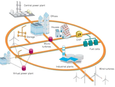
European Commission’s new report about future energy supply infrastructure, which is shown in Figure 1.1 [46], supports above conclusions.
Figure 1.1: Multi-source Multi-Sink System
Figure 1.1 shows a good example of multiple source and multiple sink energy infrastructure or so-called the DG system. There are offices, industrial plants and houses which have two distinct demands: electricity and heating. This is men-tioned as multiple sink or demand throughout in this thesis. In order to supply these demands there are micro-turbines, fuel-cells, wind turbines and a conven-tional central power plant. Addiconven-tionally a storage device is also available for extra flexibility in terms of energy supply. These devices must be operated optimally
CHAPTER 1. INTRODUCTION 3
otherwise potential of the system cannot be fully exploited; thus performance of the system may even got worse comparing to the current infrastructure.
The technology tries to create alternative energy sources for a single demand because at the moment there is no perfect solution for energy problems related to climate change. Fossil fuels will be depleted in the future and also machines using fossil fuels create unacceptable amount of harmful emissions. On the other hand, renewable energy provides a clean and unlimited energy source, however, their intermittent nature makes them unreliable. Also their energy conversion efficiencies still not comparable to systems that utilizes fossil fuels. In order to overcome these obstacles, using different kind of energy sources, multi-source, can be considered as a solution since, by this way energy supply flexibility can be increased which given an opportunity to operate devices on their most efficient zones or maximize usage of renewable energy sources.
In [22], different kinds of energy demands and sources are written as a set of equations coupled with an efficiency matrix of the devices. It can be seen that this matrix is non-invertible thus there is a potential for optimization. However, real energy systems are far from deterministic, as written in [22], and features a lot of stochastic parameters like unit cost of oil, energy demand of a house. Thus fully exploiting the potential advantages of a multi source system can be challenging.
In summary, the energy management problem involves finding mechanisms to manage devices included in the selected infrastructure at their optimal power levels based on a constructed performance index while satisfying the customer comfort level. These devices can vary from system to system and their numbers can increase or decrease but purpose of the energy management problem is the same: Finding the optimal power split between multiple sources to supply the demand.
CHAPTER 1. INTRODUCTION 4
1.2
Background and Literature Review
In this section, a background information is given on the energy management problem (EMP) from different industries.
First subsection starts with automobile EMP since it is a well-defined problem with more than a decade research. Following subsection includes definition of the residential EMP and research made on this area. Finally EMP discussion is extended for mobile devices.
1.2.1
EMP for Automotive Industry
Hybrid electric vehicles (HEVs) become popular and commercialized in recent years due to their environmental performance compared to conventional vehicles. Although there are various types of HEV powertrain configurations, a typical HEV powertrain generally consists of an electric storage device which can work bidirectionally and at least one electric motor apart from typical automobile technologies like internal combustion engine (ICE), transmissions.
By addition of storage devices and secondary sources, new operating modes become available for HEVs. For instance, during the so-called HEV specific power assist mode, the electric motor and the ICE can work together to provide the torque that is requested by the driver. Similarly, in the regenerative braking mode, some of the braking energy can be captured into the electrical storage device.
These new operating modes increased the energy supply flexibility of the vehi-cle system and made it possible to achieve certain performance parameters, such as reducing fuel consumption and harmful emissions, that cannot be achieved by conventional vehicles.
However, multiple source nature of HEVs resulted a new problem in auto-motive industry which is often called as the energy management problem. In a
CHAPTER 1. INTRODUCTION 5
typical HEV, there is additional energy sources other then internal combustion engine. Energy management problem in automotive industry aims to find the optimal power split between these energy sources in every time step to achieve minimum fuel consumption without violating the problem constraints such as comfort of the driver. Additionally, reducing harmful emissions and maximizing battery life is also used objectives and/or constraints to the optimization problem [48, 18, 47].
Automotive energy management problem is a well defined, well studied prob-lem with more than 10 years of history. The research done until now can be roughly categorized into two main approaches [48, 18, 47].
First approach is based on engineering intuition which is often called as heuris-tic methods. Rule-based control and fuzzy logic techniques falls into this cate-gory. Main aspects of the heuristic methods are, their ease of implementation and computationally efficient operation. However, they require substantial amount of time for tuning and whole potential of the additional energy supply flexibility of the vehicle cannot be fully exploited [23, 18].
Second research category is based on optimization techniques. This category can also be divided into two which are dynamic and static optimization methods. By adopting a dynamic optimization method, a global optimum can be found via dynamic programming (DP) methods or local optimums can be achieved by short-term drive cycle predictions. DP requires whole drive cycle in advance thus cannot be implemented real-time and local optimization techniques, that includes model predictive control (MPC), requires high computational resources. Static optimization methods on the other hand, does not consider future and make decisions at each time step instantaneously according to a pre-defined cost function. [23, 18].
According to [18], one of the best results for automotive energy management problem are obtained by applying dynamic optimization methods. By using these methods, performance results close to a global optimum can be obtained. However as a trade-off, computational burden and real-time implementation can be problematic. In this thesis, a residential energy management problem will be
CHAPTER 1. INTRODUCTION 6
solved by using the dynamic optimization problem and method, previously done and successfully applied in the automotive sector [35].
1.2.2
Residential EMP
Household energy consumption is an area that can not be disregarded in planning the energy future. Only in US there is more than 105 million dwellings and their energy need covers a substantial amount in US energy consumption map [39].
Generally, a residential environment requires two kinds of demand which are electricity and thermal energy. This is one of the main differences with automotive EMP in which demand is single: the torque requested from driver. In a residential area, electricity is required to power household appliances used daily such as TV, hair-dryer or kettle. Thermal power is needed for space heating and hot water demands.
Current infrastructure that supplies the demands of a dwelling generally con-sists from a national electricity grid and a gas-fired boiler. Grid electricity is obtained from big central plants which generally uses an obsolete technology thus emits substantial amount of harmful gases. Also these big power plants are established far away from the settlements due to size issues, environmental concerns and desire to lower transport costs for raw materials. So electricity pro-duced in these power plants have to be transported for long distances to reach residential areas which causes substantial amount of transportation losses. On the other hand, required thermal power from the occupants is generated inside the house by a boiler which uses natural gas connection to the building. However, the usage of a typical boiler started to become obsolete since since fossil fuel unit prices increased a lot recently and more efficient devices are developed. In this manner, it is clear that a new energy infrastructure, or at least an alternative, is needed for residential areas.
As mentioned in the beginning of this chapter, renewable energy technolo-gies are emission free but intermittent nature of them are making these sources
CHAPTER 1. INTRODUCTION 7
unreliable for residential production. For example if a dwelling is powered by solar energy, when the sun fades away there is a possibility for blackout. This problem cannot be prevented by electric storage devices because at the moment either they are not sufficient for powering consumption for long hours or satis-factory storage alternatives costs too much. In summary, the proposed energy infrastructure must also be reliable besides its efficiency and emission values.
At the moment distributed generation (DG) is the most viable candidate for household energy production. With DG there are many possibilities according to occupation type and geographical location of a dwelling. For example if it is a small family than Stirling type micro co-generation device, which is shown in Figure 1.2, can be used for electricity and thermal needs due to device’s low capacity (produces 1 kW of electricity). And if the dwelling has an acceptable amount of sunny days, than PVs or passive thermal collectors can also be used.
Figure 1.2: Micro Generation System
Figure 1.2 shows a micro co-generation system operated with Stirling engine prime mover [53]. These devices employ same principles as traditional combined heat and power cycles (CHP), which is simultaneous generation of electricity and heat. However these devices are at a size of a typical dish-washer and their output rates are scaled substantially (1-15 kW electricity production). Detail investigation of this device will be held in Section 2.
CHAPTER 1. INTRODUCTION 8
Although combining different types of technologies, as in DG, provides a great flexibility in terms of energy supply, they are harder to be efficiently operated by end-users. Thus a high level (supervisory) controller is required for optimal operation [24].
Optimal operation of the devices can be achieved by solving residential EMP which involves finding the optimal power split, according to a selected perfor-mance index, between DG sources and storage device while satisfying occupant comfort. In addition, DG sources and storage devices will likely to change a lot from one system to another since residential environment have no sizing or connection limitations like in vehicle problem. For instance, for a vehicle, size of the motor cannot be bigger than vehicle or once the vehicle is purchased no other energy sources, like another engine, can be added. So, apart from ensuring optimal operation of the energy sources, the supervisory controller must also be generic enough to be used with any device in a residential system.
Some valuable research made on operating the DG sources at residential scale in the literature. In this thesis, focus is especially on works that have used a controllable DG source, like a mCHP device. Since other devices, particularly renewable energy sources, has no prospect from the view of system dynamics and control. For instance, if the wind is available, then wind turbine is used otherwise it is turned off.
A small note before investigating current literature will be useful. In residen-tial EMP literature and in this thesis, unless mentioned otherwise, comparisons are made according to the today’s conventional case which includes a boiler for space heating and hot water demands and national grid connection for electricity demands.
Most of the systems that is investigated in the literature includes a mCHP device, an auxiliary boiler, a thermal storage and a grid connection. However most of these systems have extensions or missing devices from this configuration. Also occupancy times and climate conditions changes a lot. Thus making a healthy comparison is very difficult. However, an operational cost reduction between 5-20% is achieved with the introduction of mCHP device and a supervisory control
CHAPTER 1. INTRODUCTION 9
strategy. Control strategies that have been used in the literature can be divided into two categories which are rule-based approaches and optimization approaches based on short term prediction.
Peacock and Newborough [43] used a rule-based approach based on hybridiza-tion of time-led and heat-led control logics, which will be introduced in Sechybridiza-tion 2, and achieved an approximate 13% operational cost reduction. Besides 10% reduction in CO2 emissions also obtained. Alanne et all. [7] operated mCHP
device based on pre-determined set-points. By this way 5% reduction in CO2
emissions is achieved, however cost reductions are not given in percentage scale. Collazos et all. [17] developed a predictive optimal controller based on mixed integer linear programming (MILP) to operate residential system. A 13% reduc-tion in operating costs is achieved but no studies conducted for CO2 emissions.
Houwing et all. [25] used a model predictive controller (MPC) to minimize op-erational costs. A 5% cost reduction is obtained according to the case when no predictions are made and no further simulations are made for CO2 emissions.
1.2.3
EMP for Portable Devices
Another energy management prospect example can be given for mobile devices. Rapid development in technology made computers available to almost everyone in recent years. This fact can be seen in national consumption maps. In U.S. more than 2% of total electricity consumed by computers and internet connected devices. And this percentage is expected to increase in the following years [16]. So an effective energy management scheme is needed to keep this percentage between acceptable ranges.
Currently, most common energy management approach in computers is enter-ing these devices into sleep mode automatically while they are not used. These types of strategies generally called as dynamic power management (DPM) in the literature. By adopting DPM strategies, a power reduction between 15 to 65% is
CHAPTER 1. INTRODUCTION 10
achieved in various mobile devices [12, 13, 5]. However, with this approach, nor-mal operation of device changes and this could lead to decrease in usage comfort of consumers.
Nevertheless, there is a potential for increasing types of energy management strategies for mobile devices. In recent years, components of the mobile devices that are doing the same job started to increase. In Chapter 5 of [21], it is men-tioned that a mobile system can choose between the components that have same functionality according to their energy efficiency for that certain moment i.e. workload. For instance, wireless communication uses 990 mW while bluetooth transmission can be made only with 81 mW but wireless transmission data rate is ten times faster than bluetooth [21]. Thus, aim of the energy management prob-lem is to find optimal power split between these devices according to a desired objective.
Main objective of an energy management strategy is minimizing power con-sumption from the mobile devices, however, maximizing amount of work done in a certain time interval is also important for performance issues. So, as men-tioned in [36], besides decreasing power consumption, how much time is saved or extended for a certain work should also be considered.
Another possibility in terms of energy management is arouses for plugged-in usage of the mobile devices. In this operation mode there is two energy sources, as oppose to mobile usage, for the power required from components which are battery and electricity grid. This extra this degree of freedom for energy supply can be exploited. For example, in the time of peak consumption zones, electricity need of the device can be covered by battery. After this battery can be charged in nights when the cost of electricity is low compared to peak-zones or it can be charged when renewable energy-mix of national grid is high. By this way while electricity cost to end user can be decreased also use of renewable energy can be boosted. These type of objectives can be achieved by employing a supervisory controller which adopts an energy management strategy.
CHAPTER 1. INTRODUCTION 11
1.3
Motivation
In this thesis, a residential energy management problem will be solved based on a previously applied strategy but in a very different area; automotive engineering. The objective of this thesis is to explain that energy management problems are similar and can be solved with a baseline strategy. Thus, final part of this thesis devoted to generalization of the procedure.
The strategy applied produces a sub-optimal rule based controller that can be used in real time to exploit possibilities presented by a multi-source multi-sink system. These possibilities can be reducing operational costs, harmful emissions or dependency to fossil fuels. In this thesis, performance of the controller is evaluated in residential system. However by modifying the formulation it can be applied to any system that fits to the definition, for instance mobile devices.
1.3.1
Contributions
Contributions of this thesis are listed below;
• For all types of energy management problems, a generic formulation is cre-ated for the development of a causal sub-optimal supervisory controller. • Residential energy management problem is solved with the developed
su-pervisory sub-optimal controller, which is a novel approach in this area. • For residential energy management problem, typical energy demands cycles
are used in the simulations and all of the important performance parameters are calculated. By this way, this thesis provides a healthy data for future comparisons, in which current literature lacks at the moment.
Chapter 2
Residential Energy Management
Problem
In this chapter, first an introduction to residential energy management problem is given and possible energy supply infrastructures for the residential areas are dis-cussed. In the following section, mathematical models and energy demand cycles used in this thesis for the selected residential system are introduced. In Section 2.3, by using these models, a dynamic optimization formulation is developed and solved. In the subsequent section, a real-time supervisory controller is developed based on dynamic optimization results. Finally this chapter concluded with the simulations conducted to verify and validate the developed controller.
2.1
System Definition and Possible Frameworks
Traditionally, residential occupation areas are considered as passive energy zones which means they consume energy without any production. However, this situa-tion will likely to change with the introducsitua-tion of technologies like micro combined heat and power (mCHP) [32] and decreasing capital cost of renewable energy tech-nologies [4]. In near future, it is expected that households will produce majority of their energy needs locally and possibly use the national grid for only back-up
CHAPTER 2. RESIDENTIAL ENERGY MANAGEMENT PROBLEM 13
purposes. With an optimistic perspective, islanded operation of residential sites will also be possible in the coming years [38].
A typical house have two distinct types of energy demands. These are a thermal demand which consists from hot water and space heating needs, and an electricity demand to power household appliances. Nowadays electricity demand is supplied from a national grid which consists of big power plants and requires transmission of electricity for long distances. And thermal demand is either supplied by district heating or a small boiler fed with a natural gas connection to the house. So household units depends on outside sources for their energy needs. Alternatively, households can produce their own energy needs by a diverse set of technologies which is commonly mentioned in literature as distributed gener-ation (DG). For example when the sun is available, by using passive solar collec-tors, hot water demand can be satisfied. If the thermal needs coincides with the electric demand then using mCHP device will be cost efficient. Or sometimes a combination of these technologies can give the best solution for a selected criteria. In conclusion, a residential zone with distributed generation falls into basic def-inition of the energy management problem that is defined in the Chapter 1 and thus requiring a supervisory controller to manage these energy sources optimally. A list of commercially available technologies that can be used in residential area is given in Table 2.1.
Table 2.1: Possible Household Devices
Demand PV Sun mCHP Wind Grid Boiler Heat
Collector Turbine Pump
Thermal - + + - - + +
Electricity + - + + + -
-From Table 2.1 it can be seen that, a combination of these technologies must be used to cover both demands of a dwelling. Using only mCHP technology is possible but at the moment either operating costs more expensive than conven-tional case or capacity of the existing devices are not sufficient.
CHAPTER 2. RESIDENTIAL ENERGY MANAGEMENT PROBLEM 14
Apart from the energy converter technologies listed in Table 2.1, storage de-vices can be used to gain extra degree of freedom in terms of energy supply. For example by using an electro-chemical battery for electricity storage, one can supply the electricity demand from storage until unit price of the grid electricity decreases.
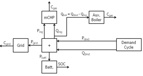
In this manner, a combination of these devices is selected for this thesis based on their availability in commercial market and their controllability. The proposed system is plotted in Figure 2.1, however the formulation that will be generated in the following sections is generic and can be applied to any residential system with the common distributed generation devices such as in 2.1.
Figure 2.1: Graphical Representation of the System Worked
In the system shown in Figure 2.1, thermal demand of the dwelling is sup-plied by the mCHP device. In addition, a conventional gas-fired boiler is also present in the system for support purposes in case mCHP device is closed or its generation capacity is not enough for the demand. Because of this, it is called as support boiler (SB). Both devices use natural gas, which is a typical connec-tion to a household, to create required heat. Electricity demand of the dwelling is covered by mCHP, national grid and lead-acid battery. Grid connection to a
CHAPTER 2. RESIDENTIAL ENERGY MANAGEMENT PROBLEM 15
house is also traditional however, battery is not a typical component in a resi-dential environment. The reason why battery is considered in the system is by the introduction of plug-in hybrid electric vehicles (PHEV), the battery will be available to house and it may be possible to use this source in a certain amount of range.
There are methods for predicting electricity demand and hot water require-ments of a house according to a chosen occupation type [54, 42]. And for de-termining space heating loads, vast number of building simulation programs are available [3]. However, in this thesis electric and thermal demands of the typical house assumed as known with respect to time and used in simulations as demand cycles. This is also a common method in automotive industry, in which drive cycle is fed to the automotive power-train controller [23, 18].
It should be noted that, the aim of the controller is not increasing the efficiency of any device depicted in the Figure 2.1, rather the objective is finding optimal power splits between these devices to achieve a certain performance index. This is expected to increase the overall efficiency of the whole system.
2.2
Mathematical Model
In this section, a mathematical model will be developed for the system proposed in Section 2.1. Since the objective is developing a supervisory controller, a simple mathematical model that accurately predicts the device outputs will be sufficient. Otherwise, optimization techniques that will be used in the following chapters will take large amount of time with an unnecessarily detailed model.
In this thesis, a modeling strategy is developed by making analogies from a common method in automotive literature which is modeling power flow with back-ward facing quasi-static approach [23, 52]. In this context, quasi-static means, power and heat demand in a certain time interval (stage) are constant. Backward-facing means power outputs of the devices are inputs for the model and output of the model blocks are required fuel for the device to create that power. An
CHAPTER 2. RESIDENTIAL ENERGY MANAGEMENT PROBLEM 16
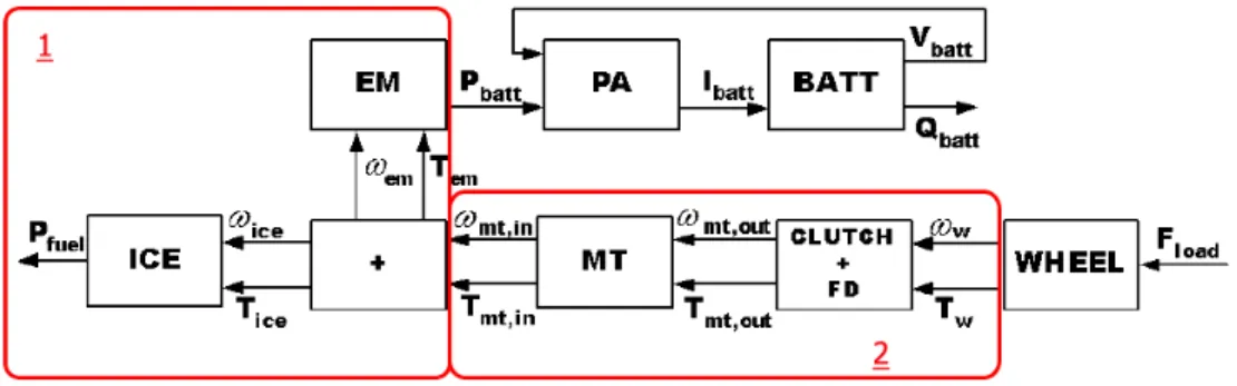
example model of this approach for a parallel HEV is given in Figure 2.2 based on [52];
Figure 2.2: HEV Backward Facing Model
The model in Figure 2.2 consists from two parts, which are selected with red triangles. First part represents different energy sources available to provide requested torque and second part is accounted for transmission losses. By using this model, the required power from energy sources can be calculated for a given load demand from the driver.
Fore residential system, second part of the model is omitted because trans-mission losses are considered negligible in distributed generation. The proposed model for the residential system proposed in Figure 2.1 is given in below Figure 2.3.
As it can be seen from Figures 2.2 and 2.3, there are some fundamental dif-ferences between models but the analogy is same which is calculating required power levels for the given demand. First significant difference is, in HEV case there is only one power flow which is required power to rotate shaft at a demanded level. In contrast, there are two different power flows, namely electric and heat in residential environment. Although these two demands from occupants are not depended, due to the devices like mCHP, production of these demands are cou-pled and solved together. Another difference is number of power sources. For instance, in home energy system there are three energy sources to provide elec-tricity demand which are national grid, mCHP and battery. On the other hand, in HEVs there is only two sources to provide requested torque which are internal
CHAPTER 2. RESIDENTIAL ENERGY MANAGEMENT PROBLEM 17
Figure 2.3: Backward Facing Model of the Proposed System
combustion engine (ICE) and electric motor with battery. Thus finding optimal power split becomes more complicated in residential problem.
In the remainder of this section, mathematical models for the devices seen in Figure 2.1 will be introduced. Also energy demand cycles for a certain occupation type will be generated to be used in optimization and simulations.
2.2.1
Converter Devices Used in the Residential System
2.2.1.1 Micro-Combined Heat and Power (mCHP)
Micro combined heat and power devices are developed in last the decade and intended to replace conventional boilers used in residential environment. The output of these devices are the same as combined heat and power (CHP) plants which is obtaining electricity and thermal energy from a single energy source (like coal or natural gas). Only power levels are much smaller compared to conventional CHP plants.
The prime-mover technologies that are used in mCHP system can be based on fuel cells, Stirling engine (SE) or internal-combustion engine (ICE). In this
CHAPTER 2. RESIDENTIAL ENERGY MANAGEMENT PROBLEM 18
thesis, ICE based devices are chosen as micro-generator for the dwelling due to their availability in the market, efficiency values (only fuel cells are more efficient then ICE but they are not commercialized yet) and ability to modulate their output power [40]. Although the created formulation is generic enough to adopt other sources.
By using the notation in [22], a micro-CHP device can be treated as single input, multiple output device. Natural gas, which is a standard connection to a dwelling, is the input for the mCHP and outputs are electricity and heat. But since the modelling approach is backward facing, these are vice-versa in the model. Graphical representation of the model is given in 2.4.
Figure 2.4: Backward facing, quasi-static representation of mCHP device Mathematical model of the ICE based mCHP device used in this thesis is based on [41]. It consists from a simple parametric model of 6 kW Cummins gas engine and it is developed according to performance data from manufacturer. This model incorporates dynamic efficiency values of the device thus permitting variable power output. The mCHP models used in the literature such as [25, 44], have only full-power and one part-load operation mode which limits controllability of the device.
In the following, mCHP model used in this thesis is investigated. First, a fraction load is defined;
CHAPTER 2. RESIDENTIAL ENERGY MANAGEMENT PROBLEM 19
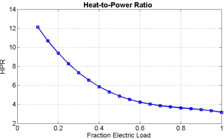
Then Heat-to-Power Ratio (HPR), which is the ratio of electricity produced over heat produced from the device, is determined by the Equation (2.2) below, which is found from a series of tests.
HP R = 18.347X3+ 45.76X2− 39.933X + 15.7 (2.2) After finding HPR, heat output of the device can be found for the required electricity output which is depicted in Equation (2.3).
Qmg = HP R.Pmg (2.3)
By using an empirical formula, specific fuel consumption of the deivce can be found as shown in Equation (2.4) which is again found from a series of tests.
SF C = 965.6X2− 1767X + 1164.2 (2.4)
Finally the model output, mass flow rate of the fuel used, can be calculated with using the Equation (2.5).
˙
mf = SF C.Pmg (2.5)
Important parameters that are used in the model are plotted in the following pages according to fraction electric load to give insight about working character-istics of the device.
In Figure 2.5, Heat-to-Power Ratio (HPR) versus fraction electrical load is plotted. It can be seen that the ratio of the heat produced from the device de-creases with respect to increase in electricity production. Therefore a calculation must be done according to the cost function at every step whether a high ther-mal production with lower electricity or a high electric and therther-mal production is needed in case of a peak consumption situation.
CHAPTER 2. RESIDENTIAL ENERGY MANAGEMENT PROBLEM 20
Figure 2.5: HPR vs. Fraction Electrical Load (X)
CHAPTER 2. RESIDENTIAL ENERGY MANAGEMENT PROBLEM 21
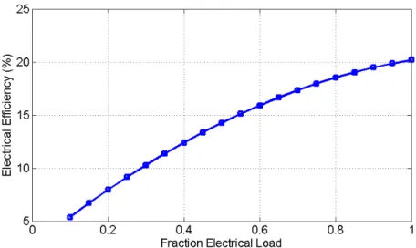
Figure 2.7: Electrical Efficiency vs. Fraction Electrical Load (X)
From Figure 2.6 and 2.7, it can be concluded that using the device in low energy zones makes it inefficient. This was an expected result, which can be concluded as characteristics of an ICE. Thus, size of the device must be selected according to the occupation type. For instance, a mCHP device with a high output , like 6 kW electricity and 15 kW thermal used in this thesis, will be too big for single-occupation type. When the device size is not selected accordingly, it will always work on inefficient zones and the cost will likely to be worse than the current infrastructure used in residential sites.
The model described here can be further improved by considering transient operation modes of the device. This type of operation characteristic occurs when the mCHP device started from cold or when it is turned off. In the former one, it takes certain amount of time to reach requested power output from the device and in the latter operation, mCHP device continues to generate power some time interval and then turns off.
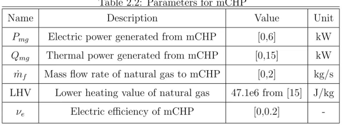
Variables and parameters used in the model equations through (2.1) to (2.5) is given in Table 2.2.
CHAPTER 2. RESIDENTIAL ENERGY MANAGEMENT PROBLEM 22
Table 2.2: Parameters for mCHP
Name Description Value Unit
Pmg Electric power generated from mCHP [0,6] kW
Qmg Thermal power generated from mCHP [0,15] kW
˙
mf Mass flow rate of natural gas to mCHP [0,2] kg/s
LHV Lower heating value of natural gas 47.1e6 from [15] J/kg
νe Electric efficiency of mCHP [0,0.2]
-2.2.1.2 Electro-Chemical Battery
As mentioned in the beginning of this chapter, battery is not a typical household gadget. However with the introduction of plug-in HEVs, the use of battery may be available for residential energy management in the future applications. Therefore a model of the battery used in parallel HEV simulations also employed in this theses.
An electrical storage battery is known to be difficult to model due to ongoing chemical reactions inside the battery which changes the terminal voltage. The approach here is based on [51], in which certain voltage values are measured corresponding to the SOC values.
From [51], change of the battery current is given in (2.6) and change of the battery state-of-the-charge is given in (2.7).
Ibatt =
Voc−pVoc2 − 4RintPbatt
2Rint
(2.6)
SOC = SOCold−
Ibattνbattt
Qbatt
(2.7)
where Vocrepresents open circuit voltage across the battery, Rintis the internal
resistance of the battery and Pbatt is either charge or recharge power of drawn/to
CHAPTER 2. RESIDENTIAL ENERGY MANAGEMENT PROBLEM 23
and (2.7) are found from current SOC value according to a pre-calculated look-up table, which can be found various sources such as [2] or could be created through measurements. For instance, the relation between SOC change and internal re-sistance of the battery used in thesis is given in Figure 2.8.
Figure 2.8: SOC vs. Battery Internal Resistance
From Figure 2.8, it can be seen that internal resistance of the battery increases while trying to charge a loaded battery. Battery resistance also increases when trying to discharge an empty battery though resistance is not high as charging case.
Besides the relations given in (2.6) and (2.7), there are also upper and lower bounds for battery state of the charge (SOC) in order to avoid degradation of the battery. In addition losses occur when charging the battery, so a constant charging efficiency of 0.9 is also included into the model.
CHAPTER 2. RESIDENTIAL ENERGY MANAGEMENT PROBLEM 24
Parameters and variables that are used in the model equations are tabulated in Table 2.3.
Table 2.3: Parameters for battery
Name Description Value Unit
Voc Open circuit voltage of battery [230,260] V
Rint Internal resistance of battery [0.3,5] Ω
(Ibatt)max Battery max. discharge current 100 A
(Ibatt)max Battery max. charging current 125 A
Pbatt Charge / Discharge power of battery f (Ibatt, Voc) kW
Qbatt Capacity of the battery 6 Ah
SOC State of the charge of battery [0.4,0.7]
-ηbatt Battery charging efficiency 0.9
-2.2.1.3 Natural Gas Fired Boiler
By using the notation defined in [22], a boiler can be considered as a single input, which is natural gas, and a single output, which is heat, system. Using the backward facing approach, graphical representation of the natural gas fired boiler can be showed as in Fig. 2.9.
Figure 2.9: Backward facing, quasi-static representation of boiler
Traditionally, Higher Heating Value (HHV) of the combustion source, in this case natural gas, is used for calculating the efficiency of a boiler [8, 10]. HHV quantity assumes that water, which is the by-product of the combustion process, is in liquid state that can also be used in heating duty.
CHAPTER 2. RESIDENTIAL ENERGY MANAGEMENT PROBLEM 25
Another important property of the boilers that influences the mathematical model is their transient operation. Boilers reach steady-state much faster than mCHP devices [53]. So warm-up and shut-down periods of the boiler can be neglected and a steady-state efficiency is used in the formulation. Efficiency value is selected based on the available commercial devices.
The mass flow rate of the fuel used by the boiler is calculated via the Equation 2.8 which is in the line with [29].
˙ mf =
Qboil
ηb.HHV
(2.8)
where Qboil to be determined from optimization algorithm.
Parameters used in the model are given in Table 2.9. Table 2.4: Parameters for battery
Name Description Value Unit
(Qb)max Max. output power of boiler 20 kW
HHV Higher heating value of natural gas 60e6 J/kg ηb Steady-state boiler efficiency 0.89
-2.2.1.4 National Grid
It is assumed that, when supervisory controller requires a certain amount from grid, it is obtained in exact amount with no delays. Because grid dynamics are much faster according to our simulation time, thus neglected.
CHAPTER 2. RESIDENTIAL ENERGY MANAGEMENT PROBLEM 26
2.2.2
Energy Demand Cycles
As mentioned in the beginning of this chapter, demands of the dwelling will not be calculated directly or simulated via a building simulation program. Instead, a set of representative demand cycles for certain occupation types will be used which are found from previous measurements conducted by International Energy Agency (IEA) Annex 42 program [11].
One of the dominant parameters affecting the performance of the proposed system is total amount of demand from the dwelling. According to occupancy type, appropriate capacities for the multiple sources should be selected, otherwise controller developed will not give better outcomes from conventional system due to sizing problem. However, the sizing problem is beyond the scope of this the-sis. Therefore appropriate capacities for the devices are chosen for the selected occupation type which is given in detail in the following paragraphs.
The electricity and Domestic Hot Water (DHW) demand cycles of a typical EU dwelling in January are given in Figures 2.10 and 2.11.
CHAPTER 2. RESIDENTIAL ENERGY MANAGEMENT PROBLEM 27
Figure 2.11: DHW demand profile throughout a day [31]
The graphics in Figures 2.10 and 2.11 are generated based on the data from [31]. Both consumption data are measured in 5 minute intervals and it shows high consumption demand according to Annex standards. The high consumption demand cycle represents a family with 5 children [31]. Although it looks like an extreme case, it is selected since the model used for mCHP has relatively higher output than other commercially available mCHP products, thus requiring a larger family for an efficient operation.
Last demand cycle for residential system is for SPace Heating (SPH) demand, which is plotted in Figure 2.12.
The Figure 2.12 shows space heating demands of a typical EU dwelling in a bright winter day. Data measured in Germany between 15 minute intervals. For consistency with other demand data’s, these 15 minutes data points are assumed as constant for three 5 minute intervals. As mentioned in the beginning, one can use building simulation programs to derive similar SPH demand cycles. However, for the scope of this work a typical SPH data like in Fig. 2.12 is sufficient.
CHAPTER 2. RESIDENTIAL ENERGY MANAGEMENT PROBLEM 28
Figure 2.12: SPH demand profile throughout a day [9]
2.3
Optimal Trajectory Generation
As mentioned in Chapter 1, dynamic optimization techniques will be used to solve residential EMP. Main advantage of dynamic optimization methods is possibility to consider the dynamic nature of the system components.
A dynamic optimization problem can be solved by a technique called Dynamic Programming (DP) [14]. This method allows non-linearity in dynamic models and also constraints within the mathematical formulation of the problem. One of the main advantage of the DP method is, it guarantees global optimum solution for the system since optimization is made for entire time horizon, not for an instant time or a small predicted time interval. The method relies on Bellman’s theory, Principle of Optimality. According to principle of optimality, if a trajectory is optimal, then every sub-trajectory must also be optimal [14].
Main disadvantage of the DP is if the system order increases, computational time increases exponentially. Thus it is not possible to use very detailed models in DP. This is known as the curse of dimensionality [14, 35].
CHAPTER 2. RESIDENTIAL ENERGY MANAGEMENT PROBLEM 29
By using DP method, optimal trajectories for the states and control inputs will be obtained. However, real-time implementation of DP is not possible since it requires future demands in advance for computation. So the optimal trajectories found from DP will be used for extracting implementable causal control rules.
Block diagram for the DP procedure is adopted from [14] and given in Figure 2.13.
Figure 2.13: DP Procedure
In Figure 2.13, ”x” represents state of the system, ”u” represents control inputs, ”w” is random parameters and µ is the control policy. By applying closed-loop optimization, controller can make appropriate reaction to the unexpected states that are developed since current information of the system, i.e. state of the system, is fed to the DP algorithm. Also energy demand requirements of the occupants are assumed as known, which are given in subsection 2.2.2. This means random parameters of the residential system, w, is known which results a deterministic problem.
Due to the curse of dimensionality, battery state-of-the-charge (SOC) chosen as only state variable. This is in the same line with the backward facing model developed in Section 2.2, with battery being the only dynamic block and other sources modelled as quasi-static. On the other hand, two control inputs are defined for the power-split approach. The two level representation of the power split algorithm used in this work is given in Figure 2.14.
CHAPTER 2. RESIDENTIAL ENERGY MANAGEMENT PROBLEM 30
Figure 2.14: Power Split Method
The ”power-split” approach used in this thesis is a common method in au-tomotive industry [35, 52, 23]. With this approach, instead of separately deter-mining the operation modes and associated power levels of electric motor and engine, a power split ratio is defined. Power split ratio couples this two sources by dividing power level of a one source to the total power requested by the driver. By this way DP only calculates this ratio and power level of these two sources extracted from it.
For residential problem, this power-split algorithm is extended into two layers. In the first split, the aim of the DP algorithm is determining battery operation mode for the current demand from the occupants. According to this decision, battery can be turned-off for the corresponding time interval or some portion of the requested power can be supplied by battery. If DP algorithm decides that battery needs a recharge, then more power must be generated from power de-mands of the occupants. Amount of the power requested is updated according to battery contribution, which is shown with Pgen. In the second split, DP algorithm
decides that how much of the required power generation, Pgen, is taken from grid,
Pgrid, and mCHP, Pmg. By using this power split-method, instead of calculating
three control inputs, for battery, mCHP and grid, only two control variables are calculated.
CHAPTER 2. RESIDENTIAL ENERGY MANAGEMENT PROBLEM 31
It should be noted that, the decisions are not made isolated. All possible power levels for the devices are generated from this power-split algorithm, then the combination that minimizes the constructed cost function is selected.
Finally, to solve problem numerically, mathematical model of the system is discretized on a state and time grid. DP procedure starts with solving the sub-problem which includes only last stage, then it extends to last two stages, last three stages and until the beginning.
A mathematical formulation developed is written according to formal standard representation which can be found in [14].
Cost function: J (~x(k), ~u(k)) = min ~ u [GN(~xN) + N −1 X k=1 L(~x(k), ~u(k))] (2.9) xk+1 = f (xk, uk) + xk (2.10) x = [0.4, 0.7] (2.11) x0 = 0.55 (2.12) xN ≥ 0.55 (2.13) u1 = [−1, 1] (2.14) u2 = [0, 1] (2.15) Ts= 5 min (2.16) N = (24 ∗ 60)/T s (2.17)
As mentioned earlier, only one state variable, ~x, is defined for the system which is battery SOC. It is assumed that battery starts to the day with a half full of charge (i.e 0.55), Eq. (2.12). Upper (i.e 0.7) and lower (i.e 0.4) bounds for the battery SOC is defined in Eq. (2.11) to prevent battery from depletion and overcharging, since they decrease battery life. These operational bounds are consistent with the literature [51], and increasing the operation zone of the battery will shorten its life-span besides it will have a small contribution to the overall efficiency of the system since the battery size is relatively small. As mentioned
CHAPTER 2. RESIDENTIAL ENERGY MANAGEMENT PROBLEM 32
in the beginning of this chapter, a plug-in HEV battery used in this residential system for future references which has a capacity of 6 Ah that is small compared to traditional batteries used in residential systems which generally have a capacity around 25 Ah [28]. Finally, for the numerical solution, the area formed from upper and lower bounds is discretized with 1001 steps. This number is found from convergence analysis which is given in Appendix A.
Function G represents the final cost, which is not required in this system since the final state of the battery is already constrained with Eq (2.13) thus depletion of the battery in the end of the simulation is not an option. Cost function L and state equation f, which represents change of the state according to time, is given in equations (2.19) and (2.20).
Power splits in Figure 2.14 are represented with ~u. First power split requires negative values for the battery recharge mode. Since they are ratio, they have an upper bound of 1. Control input domains are divided into 101 equal spaces in grid map. This number, again, obtained through a convergence analysis which is given in Appendix A. The power split algorithm is given in equations from (2.21) to (2.25).
The demand cycles generated in subsection 2.2.2 was obtained 5 minute in-terval measurements, thus simulation time Ts is selected as 5 minutes. Dynamic
optimization will be performed over a full day which is in total 1440 minutes. Dividing this value to simulation time will give optimization horizon, N, which results 288 stages.
CHAPTER 2. RESIDENTIAL ENERGY MANAGEMENT PROBLEM 33
GN(xN) = 0 (2.18)
L(~x(k), ~u(k)) = ˙mf uelCf uel+ PgridCgrid (2.19)
f (xk, uk) = − Ibattηbattt Qbatt (2.20) ˙ mf uel = f (Pmg, Pboiler) (2.21) Pbatt = u1Pdmd (2.22) Pgen = (1 − u1)Pdmd (2.23) Pmg = u2Pgen (2.24) Pgrid = (1 − u2)Pgen (2.25)
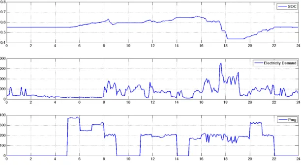
This DP formulation is solved by using a toolbox software developed by the Swiss Federal Institute of Technology, Institute of Dynamic Systems and Control [50]. This software provides a MATLAB function that can solve deterministic DP problems. The developed formulation is generic, function requires only model equations and the objective function. Then it solves the discrete-time optimal control problem automatically by using Bellman’s Principle of Optimality. It is a well coded program which results a fast computational time and can be downloaded for free from the Institute website. However the software requires solid knowledge of DP algorithm, System Theory and MATLAB programming, thus it is not easy to handle for novice users. Obtained optimal trajectories from the formulation given in Eq. (2.9) thru. (2.17) by using this software is given in Figure 2.15.
Jenkins et. al. [28] states that a battery can be used to cover peak demands from the occupants. From Figure 2.15, it can be seen that DP algorithm follows this statement and tries to discharge the battery in the evening zone when demand of the dwelling is high. Also battery charging sequences coincide with mCHP operation. For instance, between 6-8 a.m. battery is in charging mode since mCHP device is open while battery is off at 10 a.m. since mCHP is not working. This was an expected result since electricity provided from this device is an additional free power alongside its thermal power generation, which can be used to charge the battery.
CHAPTER 2. RESIDENTIAL ENERGY MANAGEMENT PROBLEM 34
Figure 2.15: Optimal State Trajectory
By using optimal control inputs, in other words power splits, the trajectories obtained for the energy sources is given in Figure 2.16.
From Figure 2.16, it is clearly seen that mCHP is a thermal device. While it supplies large amount of the thermal demand of the house, it contributes a small amount to the electricity generation. DP algorithm turns the device off when there is no thermal demand in other words heat to power ratio of the house is zero or small. This makes sense since production of electricity from mCHP device is expensive according to grid electricity, if the generated heat will not be used. From this figure it can also be concluded that besides optimal part load values, mCHP device will work three times during the day while it works only two times with a time-led controllers. This implies better utilization since extra electric power can be generated with mCHP which can decrease operational cost at the end of the day.
CHAPTER 2. RESIDENTIAL ENERGY MANAGEMENT PROBLEM 35
Figure 2.16: Optimal Usage of Devices Throughout the Day
2.4
Real-Time Supervisory Control
The aim of the controller is to enhance the system performance. The proposed system shown at the beginning of Section 2, Figure 2.1 can perform without an external, supervisory controller, by manual operation of each component by the residents of the house. But by adopting a supervisory controller, which coordi-nates the operation of the devices, system performance can be increased. This is the motivation for controller development.
Current commercial control strategies involving a mCHP device generally adopts heuristic control methods, in particular an approach called ”time-led” [53, 43]. In time-led strategy, mCHP system works with an internal controller which opens the device automatically before the occupation time. The occupa-tion time is set manually by the end user. In this manner, the mCHP device reaches steady-state and works in full power when demand is increased in other words when the occupation begins. This type of a strategy uses the mCHP de-vice only two times in a day, morning and evening intervals. So the advantages of the machine cannot be fully exploited. For instance, when the thermal demand exceeds the electric demand, which can happen at any time during the day, it is
CHAPTER 2. RESIDENTIAL ENERGY MANAGEMENT PROBLEM 36
very beneficial to use this device. In conclusion, a supervisory controller with a new rule set can increase the system efficiency significantly.
In order to determine optimal power split between sources, a dynamic opti-mization procedure is done in the previous section. Dynamic optiopti-mization gives, for a specific demand, optimal power split values for the devices. However, since DP makes decisions not isolated with one stage but considering the future, glob-ally optimum results found from DP cannot be used in real-time because algo-rithm requires whole demand information for the selected period, in advance. So a new control algorithm that can work on real-time must be developed.
In real-life applications, controller will only fed with current demand infor-mation and battery SOC level. By considering only these parameters, controller should make power splits between multiple energy sources.
A new control algorithm will be developed based on DP results. DP optimal trajectory maps will be analysed to create implementable rules. The aim here is to find effective decisions in real life when similar demands occur. DP algorithm considers and calculates many parameters to make decisions but sub-optimal decisions can be obtained by considering available parameters to the controller in real life.
2.4.1
Creating Rules
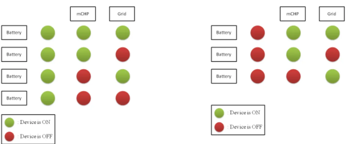
First step for creating implementable rules is determining all possible operation modes of the residential system. In Figure 2.17, a possible set of operation modes for a residential system is generated.
From Figure 2.17, which respects the power split algorithm shown in Figure 2.14, the controller must determine the battery operation mode firstly. Than according to this mode, states of mCHP device and grid electricity is decided.
In order to make decisions for the battery operation mode, DP decisions is studied. Thus, battery operation modes plotted against electricity demand from
CHAPTER 2. RESIDENTIAL ENERGY MANAGEMENT PROBLEM 37
Figure 2.17: Operation modes for residential system the dwelling in Figure 2.18.
From Figure 2.18, operation of the battery cannot be distinguished especially when demanded power level is below 2000 W. It can be concluded that the elec-tric power demand level is not only the dominant parameter when making this decision.
Here, engineering intuition suggests that when battery SOC low, it should be charged and when battery SOC is high, it should be discharged. This can be seen from the simulations as well. So current SOC level of the battery also plays an important role in making decisions apart from electricity demand of the dwelling. Therefore, a surface is created for determining first power split of the system which is between battery and remaining energy sources which is plotted in Figure 2.19.
In real-time operation, controller benefits from the surface shown in Figure 2.19. This surface is created in MATLAB surface fitting tool with R2 = 0.97.
According to current electricity demand from the house and battery feedback data SOC, amount of power that will be generated with multiple sources is determined from this surface which is denoted as Pgen. The difference between the electricity
CHAPTER 2. RESIDENTIAL ENERGY MANAGEMENT PROBLEM 38
Figure 2.18: Battery Operation with respect to Electricity Demand
CHAPTER 2. RESIDENTIAL ENERGY MANAGEMENT PROBLEM 39
Pgen= 238.7 + 0.9587Pdmd− 0.313.9SOC (2.26)
Pbatt = Pdmd− Pgen (2.27)
Similar approach is taken for second split in Figure 2.14 to find proper power split values between national grid and mCHP device. The surface fitted is given in Figure 2.20.
Figure 2.20: Power Split between Electricity Grid and mCHP
The supervisory controller uses this surface shown in Figure 2.20 to find power to be taken from electricity grid. This surface is created in MATLAB surface fitting tool with R2 = 0.98. According to the total amount of power to be
generated, Pgen, and thermal power required from users, Pth, electricity that will
be taken from national grid, Pgrid, can be found from Equation (2.29). As it can be
seen from this figure, a 2-D curve fit can also be obtained for Pgrid however as seen from Figure 2.16, mCHP operation strongly correlated with thermal demand. It is seen that including this parameter to the rule generation increases the tracking capability of the controller.
CHAPTER 2. RESIDENTIAL ENERGY MANAGEMENT PROBLEM 40
Pgrid = −5.813 + 1.008Pgen− 0.071Pth (2.28)
Pmg = Pgen− Pgrid (2.29)
At the specific stage and corresponding SOC of battery, demand values from occupants, supervisory controller can found sub-optimal operation points for the battery, mCHP and the amount of electricity to be taken from national grid by using Equations (2.26) to (2.29).
2.4.2
Charge-Sustaining Strategy
The implementable rules developed above does not consider battery constraints. Because of this, battery can be depleted or overcharged depending on the real world applications. This problem can also be seen in references [35, 52]. So, an additional rule set is required to keep battery between desired SOC levels.
The battery prevented from depleting or overcharging by a simple rule set. If the battery SOC comes near to lower bound, the first power split replaced by a rule that charges battery a certain amount. Similarly, if the battery SOC approximates to upper bound, first power split overrode by a rule that discharges battery a certain amount according to current SOC level.
This algorithm is given in equations (2.30) to (2.34).
if (SOC > SOCmax) (2.30)
Pbatt =| 0.7 − SOC | 100 × 175 (2.31)
if (SOC < SOCmin) (2.32)
Pbatt = − | SOC − 0.4 | 100 × 200 (2.33)
CHAPTER 2. RESIDENTIAL ENERGY MANAGEMENT PROBLEM 41
The battery used in the system approximately drops 1% of SOC when dis-charges 175 Watt between the selected upper and lower operation bounds of 0.7 and 0.4 respectively. The amount of total discharge required when the battery reaches upper bound is determined by the amount of SOC difference. If the difference big, more extreme cautions are taken which means more power is dis-charged. Since SOC is a fraction, it is multiplied with 100 to obtain a coefficient. The value 175 Watt increases to 200 Watt when battery reaches lower bound. This is because battery needs charging when it reaches to lower bound and due to charging efficiency more power is needed. After the new value determined for the battery power, remaining power to be generated is updated which is shown in Equation (2.29).
This subsection concludes the development of supervisory controller for resi-dential EMP. The control flow for this case is given in Figure 2.21.
CHAPTER 2. RESIDENTIAL ENERGY MANAGEMENT PROBLEM 42
In this strategy, supervisory controller is fed with current states of the dom-inant parameters and demand of the users. According to these values and gen-erated surface fit maps in Figures 2.18 and 2.19, set-points for the sources are determined. An example of this control strategy shown in 2.21 is given in Ap-pendix C as a Simulink diagram.
2.4.3
Rule Sensitivity
In the previous subsection, the sub-optimal rules for the supervisory controller created by using optimal DP results. As it can be recalled from Section 2.3, DP algorithm uses demand profiles of a typical day to find optimal trajectories for the state and control inputs. So it can be inferred that the rules generated are valid only for the selected day used in DP solution. Thus requiring the procedure for rule generation to be re-made for every day of the year.
However, it is found that demands from the dwelling is similar for seasons. For instance electricity and domestic hot water (DHW) demands for the winter season is given in Figures 2.22 and 2.23.
Figure 2.22: Average Daily Electricity Consumption in Winter
These figures are created by summing daily consumption data for the partic-ular month and then dividing it into total number of data. From the figures it can be seen that consumption data are similar in winter months, following the
![Figure 2.10: Electricity demand profile throughout a day [31]](https://thumb-eu.123doks.com/thumbv2/9libnet/5670396.113528/41.918.253.697.674.1005/figure-electricity-demand-profile-day.webp)
![Figure 2.11: DHW demand profile throughout a day [31]](https://thumb-eu.123doks.com/thumbv2/9libnet/5670396.113528/42.918.260.697.174.505/figure-dhw-demand-profile-day.webp)